CSSE2010 — Week 11 Notes
Lecture 22 — Compilation and Linking
What happens between a C program and the machine code that runs it. The note covers compiled against interpreted languages, with Java and Python’s bytecode in between; where a C compiler puts global, local and static variables; why programs are built from separately compiled object files, and the six sections of one; how the linker relocates and resolves addresses; libraries, and how a header differs from a library; and dynamic linking. It picks up from the assembler’s two passes in 2026-10-08-assembly-process. The reference note is compilation-and-linking. Where variables live is also in procedures-and-the-stack and c-language-basics, and headers against libraries in c-preprocessor-and-avr-headers.
Goals
- Tell compiling from interpreting, and place Java and Python’s bytecode and just-in-time compilation between the two.
- Say where a C compiler puts global, local and
staticvariables in the AVR’s data memory. - Explain why programs are compiled into separate object files, and what each of the six sections of an object file holds.
- Link modules by hand: lay them out in link order, relocate their internal addresses and resolve their external ones.
- Tell a header file from a library, and static linking from dynamic linking.
Compilation
A program has to be converted to machine code before it can run. The processor only fetches, decodes and executes machine instructions (fetch-decode-execute-cycle). The conversion is called compilation, and it often goes by way of assembly language: the compiler writes assembly, and the assembler turns that into machine code.
Not every program is compiled, though.
Interpretation
Some languages are interpreted, Python, Java and MATLAB among them. The high-level program is never turned into machine code. It is the input to an interpreter, a program that reads the source and carries out each statement as it reaches it. What runs on the processor is the interpreter, which is machine code like any other program. Many interpreters first turn the source into bytecode, a compact instruction format of their own, and then interpret that.
The trade-off:
- + Portability. The program is not tied to any instruction set. It runs on any machine that has an interpreter for its language.
- − Slow. Each time a statement runs, the interpreter works out again what it means, which costs many of its own instructions. In a loop it does that on every pass. A compiled program did that work once, before it started.
Java and Python
Java, and Python in the same way, takes a route between the two.
- The source is “compiled”, but into bytecode, not machine code. Bytecode is the instruction set of an imaginary machine, so it is portable across all platforms: the same file runs anywhere.
- The bytecode is the input to the Java Virtual Machine, an interpreter for bytecode, which runs on the processor.
- To recover the speed, the virtual machine just-in-time compiles the parts that run most often into real machine code while the program is running. From then on those parts run on the processor directly.
Numba does the third step for Python: it compiles a chosen Python function to machine code the first time it is called. More in compilation-and-linking.
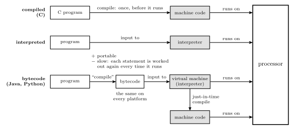
Figure 1: Three ways from a program to the processor. The grey boxes are machine code, which is the only thing a processor can run. A compiled program becomes machine code before it runs. An interpreted program never does: the interpreter is what runs, and it carries out the program’s statements one at a time, which is portable but slow. Java and Python compile to bytecode, which is the same on every platform, and a virtual machine interprets it. The virtual machine also compiles the busiest parts to machine code while the program runs, and from then on those parts run on the processor directly.
What compiling C involves
In a simplified view, compiling a C program is three jobs.
- Mapping variables to memory: giving every variable a place.
- Translating C code into assembler instructions: each statement becomes however many instructions it needs.
- Turning assembler instructions into machine code, which is the assembly process (assembly-process).
So the route is C → assembly → machine code. Some compilers go straight from C to machine code and skip the assembly text, but the jobs are the same. Job 1 is the subject of the next two sections. The whole chain from source file to flash is drawn in compilation-and-linking.
Global variables
Variables come in two kinds as far as memory is concerned. Global variables are declared outside every function. Local variables are declared inside one.
A global can be used by any function at any time, for the whole run, so the compiler gives it a fixed address in data memory. It works out the addresses itself, in the same way an assembly programmer reserves space with .dseg and .byte. On the ATmega324A the data space begins with 32 registers (addresses 0 to 31), 64 I/O registers (32 to 95) and 160 extended I/O registers (96 to 255), so the first byte free for variables is 256, 0x0100 (memory-models).
Worked: placing three globals
Where do these three globals go in the ATmega324A’s data memory, and what assembly reserves the same space?
/* global variables */
int count;
char c;
static int a;
Sizes first. On the AVR an int is 16 bits, 2 bytes, and a char is 8 bits, 1 byte (c-language-basics).
Then the addresses, one after another from 256 in the order declared. That is one layout a compiler may choose, since the order is up to the compiler.
| Variable | Size | Addresses |
|---|---|---|
count |
2 bytes | 256 and 257 |
c |
1 byte | 258 |
a |
2 bytes | 259 and 260 |
The next free byte is 261.
The assembly that reserves the same bytes:
.dseg               ; data segment: starts at the first SRAM byte, 256
count:  .byte 2     ; 256-257
c:      .byte 1     ; 258
a:      .byte 2     ; 259-260
.org 500
b:      .byte 1     ; 500
.byte n reserves \(n\) bytes and gives the first one the label’s name. .org moves the location counter, so a variable can be put at a chosen address. Here b is at 500, and 261 to 499 are left unused. That is something the assembly programmer decides. The C programmer leaves every address to the compiler.
And static? On a global, static does not change where the variable is stored: a is placed exactly like count. It makes the name private to this source file, so no other file can link to a (compilation-and-linking).
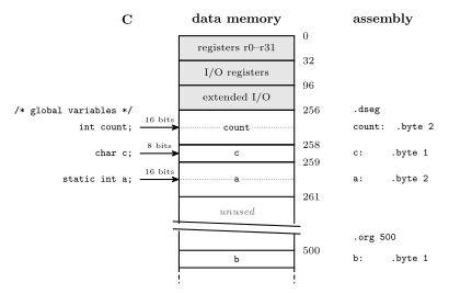
Figure 2: Three global variables placed in the ATmega324A’s data memory, with the lowest address at the top and decimal addresses on the right. The registers and the two banks of I/O registers fill addresses 0 to 255, so the globals start at 256 (0x0100). Each takes as many bytes as its type: two for an int and one for a char. On the right is the assembly that reserves the same bytes. In assembly, .org can put a variable at any address, here 500, leaving the bytes in between unused. The break in the column means the gap is not drawn to scale.
Local and static variables
A local variable exists only while its function is running. Each call gets a fresh copy, which is what makes recursion work, so a local cannot have a fixed address. It lives in the call’s stack frame instead, which holds the call’s arguments, its local variables and its return address.
When main executes call TEST, the frame for TEST is pushed onto the stack. When TEST reaches ret, the frame is popped and its locals are gone. The stack is described in procedures-and-the-stack.
The whole data memory then looks like this, from the lowest address up:
- registers r0 to r31, the I/O registers and the extended I/O registers, up to address 255;
- the globals, from 256;
- the heap, from which
malloc()hands out memory while the program runs, growing toward higher addresses; - free memory;
- the stack, which starts at the top of SRAM and grows down toward the heap. The stack pointer
SPmarks its current end, and the frames of all running calls sit betweenSPand the top.
If the stack grows down far enough to meet the heap, that is a stack overflow, and nothing stops it. This layout is drawn in compilation-and-linking.
Worked: where three variables of one function live
In this function, where is each of
a,bandcstored, and for how long?void function(void) { int8_t a; uint16_t b; static int c; ... }
ais a local, 1 byte. It is infunction’s stack frame. It is created whenfunctionis called and is gone at the return.bis a local, 2 bytes. It is also in the frame, so the frame holds 3 bytes of locals next to the 2-byte return address.cis declared inside the function but markedstatic. It is not in the frame. It lives among the globals, at a fixed address from 256 up, for the whole run. Onlyfunctioncan use the namec, but its value survives from one call to the next.
So if function is called twice, a and b start out with whatever happens to be on the stack each time, while c still holds what the first call left in it. The frame itself is drawn in procedures-and-the-stack.
Compiling C into object files
Compiling a C program runs into the same problem as the assembly process: there are names whose addresses are not yet known.
- The compiler often produces object files (
.o) as an intermediate step. Assemblers can produce object files too. - All the object files are generated first. Each of the program’s own
.cfiles is compiled, with its.hfiles and macros already expanded by the preprocessor, and the libraries arrive as object files that were compiled long ago. - Then they are all linked together, and the final details, such as memory locations, are worked out at that point.
An object file is machine code plus information. Suppose there are three source files, and the third defines a procedure TEST at its address 80. Each file is compiled as if it started at address 0, so in its object file TEST is only “80 from the start of this module”. The first file calls TEST but cannot know where TEST will end up, because that depends on where the linker puts the third module. So the object file records that the call needs TEST’s address. Once the linker has laid the modules out end to end, the third module’s start is known, TEST is that start plus 80, and the call is filled in.
Why object files
It is often useful to compile or assemble modules separately and then link them together. Change one file and only that file has to be compiled again.
The consequence is that, at compile time, nobody knows where the code will end up, meaning the addresses it will occupy. Once the location is known, the code has to be fixed. Code that carries the information needed for that is a relocatable object module. “Object module” and “object file” are used interchangeably.
The six sections of an object file
An object file is made of six sections, numbered from the bottom up. The structure is drawn in compilation-and-linking.
| Section | Holds | |
|---|---|---|
| 6 | End of module | (perhaps) a checksum to catch errors; the address at which to start execution |
| 5 | Relocation dictionary | the addresses in section 4 that need relocating |
| 4 | Machine instructions and constants | the code segment; the data segment, both initialised and uninitialised data |
| 3 | External reference table | symbols used here but defined elsewhere, and the instructions that use them |
| 2 | Entry point table | symbols defined here that other modules may use, with their addresses |
| 1 | Identification | the module’s name; where the other sections are in the file; the assembly date |
There are many different object file formats, among them a.out, COFF and ELF. ELF is what the AVR GCC toolchain produces. DWARF, often listed with them, is a format for debugging information, usually stored inside ELF files.
1. Identification section. The name of the module, the location of the other sections in the file, and the assembly date. The linker needs the locations to find everything else.
2. Entry point table. The list of symbols defined in the module that other modules may reference, with their values. The values are addresses: procedure entry points and variables. The addresses are relative to the beginning of this object module. For example, a file that defines a procedure called abs_value at address 10 lists abs_value with the value 10.
3. External reference table. The list of all symbols that are used in the module but not defined in it: procedure names and variables defined in some other module. Against each one is the list of instructions which use that symbol, the places that will need its address filled in.
4. Machine instructions and constants. The assembled code and constants, as a code segment and a data segment with both its initialised and uninitialised data. The addresses referenced in this code are not correct, because they assume the module starts at 0. They need relocation.
5. Relocation dictionary. The list of addresses of code and data in section 4 that need to be relocated. When the module is placed, a relocation constant is added to the instruction or data at each of these addresses, with different constants for code and data.
6. End of module. Possibly a checksum, to catch errors, and the address at which to start execution.
Worked: the tables for two modules
Module A defines a procedure
SUMat its address 80, and calls and jumps to a procedureX. Module B definesXat its address 71, and callsSUM. Write each module’s entry point table and external reference table.
Defined here and offered to others goes in the entry point table, with the address relative to the module’s own start. Used here but defined elsewhere goes in the external reference table, with the instructions that use it. In this example A’s call X is at 12, its jmp X at 40, and B’s call SUM at 30.
| Module | Entry point table | External reference table |
|---|---|---|
| A | SUM at 80 |
X: used by the call at 12 and the jmp at 40 |
| B | X at 71 |
SUM: used by the call at 30 |
Each symbol is defined in one module and used in the other. SUM is an entry point of A and an external reference of B, and X is an entry point of B and an external reference of A. Neither module can finish its instructions alone. The linker finishes them by matching every external reference against an entry point.
Worked: where does X end up?
Module A’s code is 100 words and its data 30 bytes. A and B are linked in the order A, then B, with code and data each starting at 0.
Xis at 71 in B. What are B’s relocation constants, what isX’s final address, and what do the instructions that useSUMandXbecome?
B’s relocation constants. B’s code goes straight after A’s code, and B’s data straight after A’s data:
- code constant = A’s code size = 100
- data constant = A’s data size = 30
The two constants differ because A’s code and A’s data are different sizes. That is why the relocation dictionary has to say, for each address, whether it is a code address or a data address.
X’s final address is its offset in B plus B’s code constant: \(100 + 71 = \mathbf{171}\).
The instructions.
- A’s
call Xat 12 andjmp Xat 40 are resolved: the linker looksXup and writes 171 into both. - B’s
call SUMmoves to \(100 + 30 = 130\) and is resolved too. A is first, so its constant is 0, andSUMstays at 80. - If B contained a branch to its own address 71, that branch would be in B’s relocation dictionary and would be relocated: \(71 + 100 = 171\). It lands in the same place, by adding a constant this time, because the target is inside the module being moved.
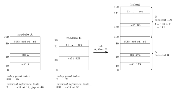
Figure 3: Two modules that each use a procedure the other defines, before and after linking, with addresses increasing up the page. Each module is assembled from 0. Its entry point table lists what it offers, with addresses relative to its own start, and its external reference table lists what it needs and which instructions need it. Linking A first and then B gives B a code relocation constant of 100, A’s size. X moves from 71 to 171, and the call and jump in A are filled in with 171. A’s constant is 0, so SUM stays at 80, and that is the address the call in B receives. The bold operands are the ones the linker wrote.
The linker and libraries
The linker combines object modules into an executable binary program, which is machine code. Each source procedure, in C or in assembly, goes through a translator (a compiler or an assembler) and becomes an object module. The linker takes all the object modules, plus whatever it needs from a library, and produces the one executable. The chain is drawn in compilation-and-linking.
A library is
- a collection of object files with an additional index, which tells the linker which member defines which symbol, and
- a collection of useful functions and procedures, ready to link.
The principle is not to reinvent the wheel, and to use library code where possible. The standard C library is the usual example. It provides:
- standard input and output,
- string handling,
- date and time functions,
- general utilities.
More in compilation-and-linking.
Header files against the library
A header file (.h) is not the library. A header file
- defines useful preprocessor macros,
- declares the functions that are in the library, as function prototypes, and
- declares the variables that are available externally, with
extern.
The library is the collection of object files that implements the functions.
A prototype tells the compiler the name, the argument types and the return type, which is enough to check a call and generate it. It contains no code. The code is in the library, and it is the linker that joins it on. The header goes to the compiler, by way of the preprocessor, and the library goes to the linker. Forgetting the header shows up when compiling, as an “implicit declaration” of the function: a warning from older compilers, an error from newer ones. Forgetting the library shows up when linking, as an “undefined reference”. See c-preprocessor-and-avr-headers.
Linking: relocating and resolving
Linking is a similar problem to assembling. It has the external reference problem: symbols are used before their values are known. A module can call a procedure in a module the linker has not read yet. So the linker needs two passes as well, in the same way the assembler does (assembly-process). The first pass places every module and collects every entry point. The second pass patches the code.
When modules are joined together, addresses need relocating or resolving.
- Relocating means adding some constant value: the module’s starting address, added to an address that points within the module.
- Resolving means finding the value of an “external” address: one that points into a different module, looked up from the entry points the linker collected.
The passes are described step by step in compilation-and-linking.
Worked: linking modules A and B
Four object modules are each assembled from 0. Module A (length 400) holds
BRANCH TO 200at 0,MOVE P TO Xat 200 andCALL Bat 300. Module B (length 600) holdsBRANCH TO 300at 0,MOVE Q TO Xat 300 andCALL Cat 500. Module C (length 500) begins withBRANCH TO 200. The modules are linked in the order A, B, C, D, after 100 words of start-up code. Where does B start, and what does each instruction of A and B become?
Where everything goes. The start-up code fills 0 to 99, so A starts at 100. A is 400 long, so it fills 100 to 499 and B starts at 100 + 400 = 500. B is 600 long, so C starts at 500 + 600 = 1100. The relocation constants are +100 for A and +500 for B.
Each instruction. An instruction at offset \(o\) in a module starting at \(s\) is now at \(s + o\).
| Now at | Was | Becomes | How |
|---|---|---|---|
| 100 | A: BRANCH TO 200 |
BRANCH TO 300 |
relocate, +100 |
| 300 | A: MOVE P TO X |
unchanged | no code address |
| 400 | A: CALL B |
CALL 500 |
resolve: B starts at 500 |
| 500 | B: BRANCH TO 300 |
BRANCH TO 800 |
relocate, +500 (100 + 400) |
| 800 | B: MOVE Q TO X |
unchanged | no code address |
| 1000 | B: CALL C |
CALL 1100 |
resolve: C starts at 1100 |
| 1100 | C: BRANCH TO 200 |
BRANCH TO 1300 |
relocate, +1100 |
Check that nothing broke. A’s branch at 100 now targets 300, which is exactly where A’s MOVE P TO X went. B’s branch at 500 targets 800, where B’s MOVE Q TO X went. A relocated branch still lands on the same instruction, because the branch and its target moved by the same amount. A call to another module is not fixed by adding A’s constant, though. CALL B needs B’s start, which only the layout of the whole program determines.
Finishing the job with D (length 300, at 1600) gives CALL D → CALL 1600 and D’s BRANCH TO 200 → BRANCH TO 1800. The complete table, and a drawing of the program after each of the linker’s two passes, are in compilation-and-linking.
Worked: where does module 2 start?
Modules are linked in order 3, 2, 1 starting at program address 62 and data address 256. At what program (code) address will module 2 start?
Module c-seg size (words) d-seg size (bytes) 1 45 17 2 67 5 3 100 25 A. 62 B. 87 C. 107 D. 146 E. 162 F. 229
Answer: E, 162.
The question asks about the code address, so only the c-seg column matters. In the order 3, 2, 1, module 3 goes first, from 62. It takes 100 words, 62 to 161, so module 2 starts at
\[62 + 100 = 162.\]
The full layout, with both memories:
| Module | Code (words) | Data (bytes) | Code constant | Data constant |
|---|---|---|---|---|
| 3 | 62 to 161 | 256 to 280 | +62 | +256 |
| 2 | 162 to 228 | 281 to 285 | +162 | +281 |
| 1 | 229 to 273 | 286 to 302 | +229 | +286 |
The next free code word is 274 and the next free data byte is 303.
Where the wrong answers come from:
- A, 62, is where module 3 starts. It is the first module in the order, not module 2.
- B, 87, is \(62 + 25\): module 3’s data size added to the code start.
- C, 107, is \(62 + 45\): module 2’s start if the modules were linked in the order 1, 2, 3.
- D, 146, matches no boundary in either memory.
- F, 229, is where module 1 starts, after module 2 rather than before it.
Why 62 and 256? On the ATmega324A, program words 0 to 61 hold the interrupt vector table, so 62 (0x003E) is the first word free for code (avr-interrupts). Data addresses 0 to 255 are registers and I/O, so 256 (0x0100) is the first byte of SRAM. Code is counted in words because each program memory location holds a 16-bit word. Data is counted in bytes because each data memory location holds one byte (memory-models).
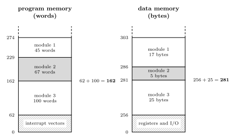
Figure 4: Three modules linked in the order 3, 2, 1, with addresses increasing up the page. Code and data are laid out separately, each in its own memory and its own units: words of program memory from 62, the first word after the interrupt vector table, and bytes of data memory from 256, the first byte of SRAM. Every module starts where the module before it in link order ends, so module 2’s code begins after module 3’s 100 words, at 162, and its data after module 3’s 25 bytes, at 281. Those two starts are module 2’s relocation constants. The heights are not to scale.
Dynamic linking
So far, all the object code, library and main program alike, is linked into one binary before the program runs. That is static linking.
Alternatively, linking can happen at run time: a library procedure is linked when it is first called. The executable contains only a reference to it, and the library stays in a file of its own. DLLs on Windows work this way.
The advantages:
- It saves space. The libraries are not linked into the binary executable, and every program that uses a library shares the one copy.
- The library can be updated independently of the programs that use it, and a fix reaches all of them without relinking.
The second is also a disadvantage. A program can break because something else installed a different version of a DLL it depends on. On earlier versions of Windows this happened often enough to be called “DLL hell”.
An AVR program has no operating system to do the run-time linking, so everything is linked statically. The two are compared side by side in compilation-and-linking.
See also
- compilation-and-linking — the reference note: the toolchain, variables in memory, the object file, both passes of the linker, libraries, dynamic linking
- assembly-process · 2026-10-08-assembly-process — the assembler’s two passes, the problem the linker repeats one level up
- procedures-and-the-stack — stack frames,
call,ret, push and pop - c-language-basics — how big each type is, and where globals, locals and statics live
- c-preprocessor-and-avr-headers —
#include, macros, and the header against the library - memory-models · avr-interrupts — the data map from 256 and the vector table that ends at 61
- 2026-10-19-floating-point-numbers — Lecture 23
Reference material
The Assembly Process
How an assembly language program becomes machine code. It covers the four fields of a statement, the directives that tell the assembler what to do as opposed to the CPU, the three memory segments of the AVR and the location counter that walks through each, and the two-pass assembler with its symbol table, which is how a program can jump to a label it has not reached yet. The program skeleton these pieces fit into is avr-program-structure, and the memories the segments map onto are in memory-models and avr-architecture. First met in 2026-10-08-assembly-process.
What an assembler does
An assembler turns a text file of assembly language into the bits that go into the chip’s memories. Most of that is translation, one statement at a time: add r1, r2 has a fixed binary form, 0000 1100 0001 0010, and nothing else in the file can change it (avr-instructions). Each instruction becomes exactly one machine instruction (instruction-set-architecture).
Two things make it more than a lookup table:
- A program is more than instructions. It has to say where things go in memory, reserve space for variables, put constant tables in flash and give registers and addresses readable names. None of that is an instruction for the CPU. These lines are directives, commands to the assembler itself.
- Names stand for numbers that are not known yet.
jmp RESETneeds the address ofRESET, and ifRESET:is further down the file, a single read from top to bottom cannot supply it. The cure is to read the file twice.
C reaches machine code by a different road: the compiler turns one line of C into many instructions (2026-09-07-introduction-to-embedded-c-programming), and how that output is joined into a program is compilation-and-linking.
The format of a statement
An assembly program is a sequence of one-line statements. A statement has up to four fields, and any of them may be empty:
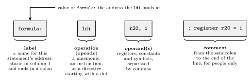
Figure 5: The four fields of one assembly statement. The label names the address this statement ends up at, so other statements can jump to it or refer to the data there. The operation field holds the mnemonic, which is either an instruction for the CPU or, if it starts with a dot, a directive for the assembler. The operands are what the operation works on: registers, constants or symbols, separated by commas. The comment runs from the semicolon to the end of the line and is thrown away by the assembler.
Label. A name for a position in memory. Labels exist so that statements can be jumped to and so that data can be referred to by name. Its value is the address the statement lands at: a word address in program memory for code, a byte address in data memory for a variable. By convention a label starts in column 1 and everything else is indented, so labels stand out down the left edge. In AVR assembly it ends with a colon.
Operation. A symbolic abbreviation for an instruction’s opcode, a mnemonic: LDS for Load Direct from data Space, ldi for load immediate. Or a directive, which starts with a dot.
Operands. The registers and addresses the instruction uses. Register names belong to the machine:
| Machine | Register names |
|---|---|
| Pentium | eax, ebx, esi, edi, … |
| SPARC | o0..o7, i0..i7, l0..l7, g0..g7 (out, in, local and global) |
| AVR | simply r0..r31 |
An address operand is usually written as a label, lds r16, count, and the assembler substitutes the number.
Comment. Space for explanation, only for people: the assembler discards it. In assembly comments are not optional politeness. ldi r20, 13 says nothing about why; the comment is the only place the intent is written down.
Ending a statement. Some assemblers want a semicolon at the end of every statement and others do not. AVR assembly does not: the end of the line ends the statement, and a semicolon starts a comment.
Directives
Besides instructions, the assembler needs other information, for example:
- where in memory the code and data should go;
- nicer names for registers and addresses, such as
tempforr16orSPHfor I/O address0x3E; - space for variables and tables of constants.
That information is given as a directive, also called a pseudo-instruction: a command to the assembler itself, written where an instruction would be and preceded by a dot, as in .byte or .def temp = r16. Most directives produce no machine code at all. They change what the assembler knows or where it is putting things.
The assembler in Microchip Studio, AVRASM2, has these, among others:
| Directive | What it does |
|---|---|
.byte |
reserve bytes for a variable |
.cseg |
switch to the code segment |
.csegsize |
set the program memory size |
.db |
define constant byte(s) |
.def |
give a register a symbolic name |
.device |
name the exact processor the program is for |
.dseg |
switch to the data segment |
.dw |
define constant word(s) |
.equ |
set a symbol equal to an expression, permanently |
.eseg |
switch to the EEPROM segment |
.exit |
stop processing this file |
.include |
read source from another file, here |
.list, .nolist |
turn generation of the list file on, off |
.listmac |
show macro expansions in the list file |
.macro, .endm (or .endmacro) |
begin, end a macro |
.org |
set the location counter: the address of what comes next |
.set |
set a symbol equal to an expression, changeably |
.if, .else, .elif, .endif |
conditional assembly: include lines only if a condition holds |
All of this is AVRASM2’s syntax. Other assemblers, even ones for the AVR, spell things differently. The GNU assembler used behind avr-gcc has a .byte directive too, and there it stores the bytes listed instead of reserving space.
Segments and location counters
The AVR has three memories (avr-architecture), and to the assembler each is a segment. Directives choose which segment the following lines go into:
| Segment | Directive | Memory | What can go there |
|---|---|---|---|
| code | .cseg |
flash, program memory | instructions, and constant data |
| data | .dseg |
SRAM, data memory | space only, reserved for variables |
| EEPROM | .eseg |
EEPROM | constants |
The data segment cannot be given values. The assembler’s output is programmed into flash and EEPROM, which keep their contents with the power off. SRAM is empty at power-up and holds nothing until the running program writes to it, so all the assembler can do there is decide which addresses each variable will use.
Each segment has its own location counter: the address the next thing in that segment will be placed at. A label takes the current value of its segment’s counter, and every statement that places something advances the counter by its size. Switching segment does not reset anything. It only changes which counter is in use, so a segment can be built up in pieces, and each piece carries on where the last piece of the same segment stopped.
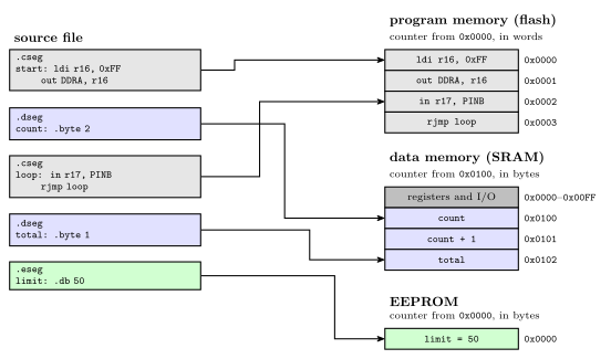
Figure 6: One source file feeding three memories. The file switches segment four times, and each piece goes to the memory its directive names, carrying on from where the previous piece of the same segment stopped: the second code piece follows the first in flash, and total follows count in SRAM. Each segment has its own location counter. The code counter starts at 0 and counts 16-bit words. The data counter starts at 0x0100, the first address after the registers and I/O, and counts bytes. The EEPROM counter starts at 0 and counts bytes. Grey marks code, blue data and green EEPROM.
Where each counter starts:
- Code: at 0, the reset address, and the assembler starts in the code segment, so a file with no segment directives is all code. The counter counts 16-bit words, because each program-memory address names a word (memory-models).
- Data: at the first free SRAM address,
0x0100on the ATmega324A, since0x0000to0x00FFare the registers and I/O registers. The counter counts bytes. - EEPROM: at 0, counting bytes.
.org sets the counter of the current segment to a given value, so whatever follows is placed there. It works in any segment, in that segment’s units.
Reserving and defining data
Three directives put data in memory:
| Directive | Segment | Places | Size |
|---|---|---|---|
.byte n |
data | nothing: reserves n bytes |
n bytes |
.db a, b, … |
code or EEPROM | constant bytes, 8 bits each | one byte each |
.dw a, b, … |
code or EEPROM | constant words, 16 bits each | two bytes each |
.byte is allowed only in the data segment: it is how a variable gets an address. .db and .dw initialise constants, so they belong where constants can live: the code segment or the EEPROM segment.
.db in the code segment packs two bytes per word. Program memory is 16 bits wide, so consecutive bytes share a word, the first in the low byte and the second in the high byte. A .db line with an odd number of bytes leaves half a word over, and the assembler fills it with a zero pad byte so that the next line starts on a whole word. Each .db line is padded on its own, so two 5-byte lines take 3 words each, not 5 words between them. AVRASM2 warns when it pads. Writing the 0 yourself gives the same layout without the warning.
.dw takes one whole word per value, so it is the natural way to store numbers bigger than 255, or addresses.
Worked: a lookup table in flash
A lookup table (LUT) is a table of constants a program reads instead of computing. Lay out:
        .cseg
table1: .db  11, 12, 30
table2: .dw  100, 133
        .org 500
table3: .dw  ...
The code counter starts at 0.
table1= 0. Three bytes: 11 and 12 share word 0, 30 takes the low half of word 1, and a pad 0 fills its high half. The counter moves to 2.table2= 2. Two words, 100 at word 2 and 133 at word 3. The counter moves to 4..org 500sets the counter to 500. Words 4 to 499 are skipped, and nothing is placed there.table3= 500 (0x01F4).
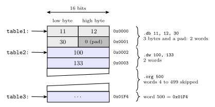
Figure 7: The lookup table laid out in program memory, one 16-bit word per row, lowest address at the top. A .db puts two bytes in each word, the first in the low byte, and pads an odd count with a zero byte so that the next label starts on a whole word: here 30 shares word 1 with a pad. Each .dw value fills a whole word. The .org moves the location counter forward and leaves words 4 to 499 untouched, so table3 lands at word 500. The diagonal break means the gap is not drawn to scale. Grey marks the .db bytes, dark grey the pad and blue the .dw words.
On the data side, two .byte 2 lines in separate .dseg pieces end up next to each other, at 0x0100 and 0x0102, whatever code sits between them in the file. That is worked in 2026-10-08-assembly-process.
Naming things: .def, .equ and .set
Three directives give a name to something. None of them places anything or moves a location counter.
| Directive | Names | Can it be changed later? | Example |
|---|---|---|---|
.def |
a register, and only a register | yes, by another .def |
.def ZH = r31 |
.equ |
a value: a number, an I/O address, an expression | no | .equ sreg = 0x3f ; Status register |
.set |
a value | yes, by another .set |
.set io_offset = 0x23 ; For now |
.equ is the usual choice for a constant, because a second definition is an error and catches a clash of names. .set is for a value that a later part of the file deliberately redefines, which is what for now in the comment above says.
Check. The same program defines .equ SPH = $3E and .def ZH = r31. Why .equ for one and .def for the other? SPH is an I/O register, which instructions such as out reach by its I/O address, 0x3E. To the assembler that is just a number, so .equ. ZH is general-purpose register r31, the high byte of the Z pointer, which instructions name as a register operand, so .def.
Two more directives are about files and the processor rather than names:
.include "file"reads another file in at that point, as if its text were typed there..include "m324Adef.inc"is howPORTA,SPH,RAMENDand the rest get defined: the file is mostly.equand.deflines (avr-io-ports)..device ATmega324Anames the exact processor. The assembler then rejects any instruction that chip does not implement..exitstops reading the file at that line. Anything after it is ignored.
The forward reference problem
Read top to bottom, most statements can be translated on the spot. add r1, r2 names two registers and nothing else, so its machine word is known at once.
A label used before it is defined is different. A program usually starts with
        jmp  RESET
        ...
RESET:  ldi  temp, low(RAMEND)
When the assembler reaches the jmp, it knows the opcode but not the operand: RESET has not been seen, so there is no address to put in the instruction. This is the forward reference problem. One forward reference anywhere in a file is enough to stop a single top-to-bottom pass from finishing the job.
The two-pass assembler
The fix is to process the file twice.
Pass one: define every symbol. Go through the file without generating anything. Keep a location counter for each segment, starting at 0 for code and EEPROM and at 0x0100 for data. For each line:
- if it has a label, enter the label in the symbol table with its segment and the current value of that segment’s counter;
- if it is
.equ,.setor.def, enter that name and its value; - if it is
.cseg,.dsegor.eseg, switch counters; if it is.org, set the current counter; - advance the current counter by the line’s size: 1 or 2 words for an instruction, the padded number of words for
.db, a word per value for.dw,nbytes for.byte n, and 0 for a line that only names something.
Pass one only needs each line’s size, and every instruction’s size is known without knowing its operands: jmp RESET takes 2 words whatever RESET turns out to be.
Pass two: assemble. Go through the file again with the counters reset. Now every symbol’s value is in the table, so each instruction can be assembled, turned into actual machine code, with its operands filled in, and each .db and .dw value can be written.
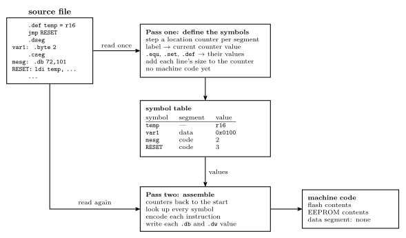
Figure 8: The two-pass assembler. Pass one reads the whole source and produces no code: it steps the location counters and records each symbol’s segment and value in the symbol table. Pass two reads the same source again from the top and, with every value now in the table, encodes each instruction and writes each constant. Its output is the contents of flash and of EEPROM. The data segment produces no output, only the addresses its labels were given.
Worked: a two-pass trace
The program:
        .equ    RAMEND = $08FF
        .equ    SPH = $3E
        .equ    SPL = $3D
        .def    ZH = r31
        .def    ZL = r30
        jmp     RESET
        .dseg
var1:   .byte   2
var2:   .byte   2
        .cseg
        .def    temp = r16
mesg:   .db     72,101,108,108,111
table:  .dw     var1, var2
RESET:  ldi     temp, low(RAMEND)
        out     SPL, temp
        ldi     temp, high(RAMEND)
        out     SPH, temp
        ...
        ldi     ZH, high(mesg*2)
        ldi     ZL, low(mesg*2)
        lpm                     ;R0 <= M[Z]
Pass one. The code counter starts at 0 and the data counter at 0x0100 (256).
- The five
.equand.deflines enterRAMEND,SPH,SPL,ZHandZLin the table and place nothing. jmp RESETis a 2-word instruction, so it takes words 0 and 1 and the code counter goes to 2.RESETis not known yet, and pass one does not need it to be..dsegswitches to the data counter.var1= 256 (0x0100) and.byte 2moves the counter to 258.var2= 258 (0x0102) and the counter goes to 260..csegswitches back to the code counter, still at 2..def temp = r16enterstemp.mesg= 2. Five bytes need three words with a pad, words 2 to 4, and the counter goes to 5.table= 5. Two words, 5 and 6, and the counter goes to 7.RESET= 7. Each of the four instructions from here is one word:ldiat 7,outat 8,ldiat 9,outat 10.
The counters run code 0, 2, 5, 7, 8, 9, 10, 11 and data 256, 258, 260. The EEPROM counter is never used.
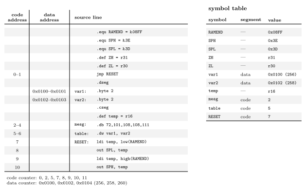
Figure 9: Pass one over the example, line by line. The two address columns show where each line is placed in its own segment, so a range means the line takes several words or bytes: the jmp two words, the 5-byte .db three words with its pad, the .dw two words, each .byte 2 two bytes. Lines that only name something or switch segment take no space and have no address. The code and data counters advance independently, which is why mesg comes straight after the jmp even though the data lines sit between them in the file. On the right is the symbol table pass one leaves behind: every name, the segment its value belongs to, and the value. The .equ and .def names have no segment.
So the instruction at RESET is at program address 7, mesg is at 2, table at 5, and the variables at 256 and 258.
Only one reference in the program is forward: jmp RESET. Every other symbol (RAMEND, var1, var2, mesg, SPL, SPH, ZH, ZL, temp) is defined above the line that uses it. One is enough to need the second pass.
Worked: what pass two writes
With the table complete, pass two replaces every symbol by its value and encodes:
| Address | Statement | With symbols replaced | Machine word(s) |
|---|---|---|---|
| 0–1 | jmp RESET |
jmp 7 |
0x940C 0x0007 |
| 2–4 | .db 72,101,108,108,111 |
bytes 72, 101, 108, 108, 111 and a pad 0 | 0x6548 0x6C6C 0x006F |
| 5–6 | .dw var1, var2 |
.dw 0x0100, 0x0102 |
0x0100 0x0102 |
| 7 | ldi temp, low(RAMEND) |
ldi r16, 0xFF |
0xEF0F |
| 8 | out SPL, temp |
out 0x3D, r16 |
0xBF0D |
| 9 | ldi temp, high(RAMEND) |
ldi r16, 0x08 |
0xE008 |
| 10 | out SPH, temp |
out 0x3E, r16 |
0xBF0E |
| later | ldi ZH, high(mesg*2) |
ldi r31, 0x00 |
0xE0F0 |
| later | ldi ZL, low(mesg*2) |
ldi r30, 0x04 |
0xE0E4 |
| later | lpm |
lpm |
0x95C8 |
Points worth checking by hand:
ldi r16, 0xFF. The form is1110 KKKK dddd KKKK, withddddthe register number minus 16.K=1111 1111anddddd=0000, so1110 1111 0000 1111=0xEF0F.- The
.dbwords. The first byte of each pair is the low byte: 72 and 101 make0x6548. The odd fifth byte, 111 =0x6F, shares its word with the pad. low()andhigh()split a 16-bit value into its bytes at assembly time.RAMEND=0x08FFgives0xFFand0x08: this is the stack pointer being set to the top of SRAM (procedures-and-the-stack).mesg*2.mesgis a word address, 2.lpmreads one byte of program memory from the byte address in Z, and word 2 starts at byte 4. So Z =0x0004, andlpmloadsr0with the byte there, 72, theHofHello. The two kinds of address are drawn in memory-models.tableholds the two variables’ addresses,0x0100and0x0102: a table of pointers, in flash, into the data segment.
Common mistakes
- Counting
jmpas one word. It is two, because it carries a full program address (avr-branches-and-jumps).rjmpis one. - Forgetting the pad. A
.dbline with an odd number of bytes takes a whole extra word, and each line is padded separately. - Counting
.dbbytes as words. Two bytes share a word in program memory. - Letting
.dseglines move the code counter, or the other way round. Each segment has its own counter, and switching segments only chooses which one is in use. - Giving size to lines that only name things.
.equ,.set,.def,.cseg,.dseg,.includeand comments place nothing. - Expecting
.byteto store a value..byte 2reserves two bytes. It does not put a 2 anywhere. Constants go in flash or EEPROM with.dbor.dw. .deffor a constant, or.equfor a register..defis for registers only.- Redefining an
.equ. It cannot be changed; that is what.setis for. - Handing a code label straight to
lpm. A code label is a word address.lpmwants the byte address, the label times 2. - Ending statements with a semicolon out of habit from another language. In AVR assembly it starts a comment.
- Assuming another assembler reads the same way. Directive names and meanings change between assemblers, even for the same chip.
See also
- avr-program-structure — the skeleton: vector table,
RESET, the main loop, and where segments and directives go in it - memory-models — word and byte addresses, cell sizes, and the AVR’s separate address spaces
- avr-architecture — flash, SRAM and EEPROM, the three memories behind the three segments · memory-technologies — what each of the three is as a technology
- avr-instructions · avr-branches-and-jumps — instruction sizes, which decide how far the code counter moves
- avr-interrupts —
.orgplacing eachjmpin the vector table - procedures-and-the-stack — the stack pointer set-up the worked example starts with
- instruction-set-architecture — assembly as a level, one line to one instruction
- compilation-and-linking — the road to machine code from C
- 2026-10-08-assembly-process — Lecture 20
AVR Interrupts
How the ATmega324A implements interrupts, and how to write one and switch it on, in assembly and in C: the path from a device’s request to the handler and back, the vector table, the switches that decide whether a request is taken, the ISR template and its stack, ISR() and the _vect names, volatile, priority, and a complete timer-interrupt program. First met in 2026-09-21-interrupts. What an interrupt is on any CPU (polling versus interrupts, the fourteen-step sequence, transparency, nesting) is polling-and-interrupts.
The path of an interrupt
An interrupt is a procedure call the hardware makes (procedures-and-the-stack). The CPU finishes the instruction in progress, pushes the address of the next one, turns interrupts off and loads the PC with the address of the vector table entry for the source. The entry holds a jmp to the handler. The handler ends with reti, which pops the return address and turns interrupts back on.
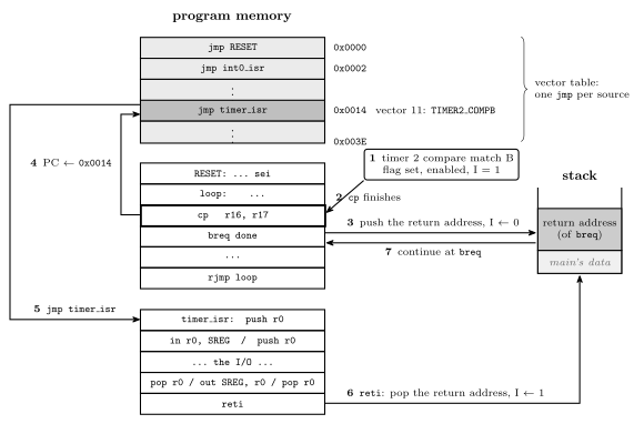
Figure 10: One timer interrupt from start to finish. The request (1) arrives while cp is executing, and the CPU lets it finish (2): an AVR instruction is never abandoned halfway. The hardware then pushes the address of the next instruction, breq, clears the I bit (3), and loads the PC with 0x0014 (4), the vector table entry for Timer/Counter 2 compare match B. The jmp stored there reaches the handler (5), which saves what it uses, does its work, restores, and ends with reti (6). That pops the return address and sets I again, and execution continues at breq (7) as if nothing had happened. It will, provided the handler restored the status register, because breq is about to read the Z flag that cp set. Nothing in the main program refers to the handler; the vector table is the only link between them.
The vector table
The first addresses of program memory hold the interrupt vector table: one entry per interrupt source, in a fixed order, each a two-word jmp to that source’s handler (avr-branches-and-jumps). The AVR uses a table of jump instructions, not a table of addresses. When it takes an interrupt it loads the PC with the address of the entry itself and executes what it finds there. So:
\[\text{entry address} = 2 \times (\text{vector} - 1)\]
RESET is vector 1, at 0x0000. A reset is taken through the same table as an interrupt, which is why every program begins with jmp RESET (avr-program-structure). The table has 31 entries on the ATmega324A and ends at 0x003C, so the program proper starts at 0x003E.
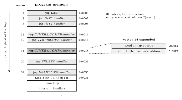
Figure 11: The bottom of program memory. Each vector-table entry is two words, the two halves of a jmp, so entry \(n\) sits at address \(2(n-1)\), and the table’s order is also its priority order: when two requests are waiting, the one nearer the top is taken first. The expanded entry shows what one of them holds, taking vector 14, Timer/Counter 1 compare match A, as the example. An entry for a source the program does not use can hold anything, as long as that interrupt is never enabled. The program itself starts at the first address after the table, which the jmp in entry 1 reaches at reset.
The full table for the ATmega324A, from pages 69–70 of the datasheet. The Group column sorts the sources by kind: GPIO, T/C, Comms, analog and system. The C name is the Source followed by _vect.
| Vector | Address | Source | Interrupt definition | Group | C handler |
|---|---|---|---|---|---|
| 1 | 0x0000 |
RESET |
RESET, watchdog reset, etc. | — | — (the program’s start) |
| 2 | 0x0002 |
INT0 |
External Interrupt Request 0 | GPIO | ISR(INT0_vect) |
| 3 | 0x0004 |
INT1 |
External Interrupt Request 1 | GPIO | ISR(INT1_vect) |
| 4 | 0x0006 |
INT2 |
External Interrupt Request 2 | GPIO | ISR(INT2_vect) |
| 5 | 0x0008 |
PCINT0 |
Pin Change Interrupt Request 0 (port A) | GPIO | ISR(PCINT0_vect) |
| 6 | 0x000A |
PCINT1 |
Pin Change Interrupt Request 1 (port B) | GPIO | ISR(PCINT1_vect) |
| 7 | 0x000C |
PCINT2 |
Pin Change Interrupt Request 2 (port C) | GPIO | ISR(PCINT2_vect) |
| 8 | 0x000E |
PCINT3 |
Pin Change Interrupt Request 3 (port D) | GPIO | ISR(PCINT3_vect) |
| 9 | 0x0010 |
WDT |
Watchdog Time-out Interrupt | system | ISR(WDT_vect) |
| 10 | 0x0012 |
TIMER2_COMPA |
Timer/Counter2 Compare Match A | T/C | ISR(TIMER2_COMPA_vect) |
| 11 | 0x0014 |
TIMER2_COMPB |
Timer/Counter2 Compare Match B | T/C | ISR(TIMER2_COMPB_vect) |
| 12 | 0x0016 |
TIMER2_OVF |
Timer/Counter2 Overflow | T/C | ISR(TIMER2_OVF_vect) |
| 13 | 0x0018 |
TIMER1_CAPT |
Timer/Counter1 Capture Event | T/C | ISR(TIMER1_CAPT_vect) |
| 14 | 0x001A |
TIMER1_COMPA |
Timer/Counter1 Compare Match A | T/C | ISR(TIMER1_COMPA_vect) |
| 15 | 0x001C |
TIMER1_COMPB |
Timer/Counter1 Compare Match B | T/C | ISR(TIMER1_COMPB_vect) |
| 16 | 0x001E |
TIMER1_OVF |
Timer/Counter1 Overflow | T/C | ISR(TIMER1_OVF_vect) |
| 17 | 0x0020 |
TIMER0_COMPA |
Timer/Counter0 Compare Match A | T/C | ISR(TIMER0_COMPA_vect) |
| 18 | 0x0022 |
TIMER0_COMPB |
Timer/Counter0 Compare Match B | T/C | ISR(TIMER0_COMPB_vect) |
| 19 | 0x0024 |
TIMER0_OVF |
Timer/Counter0 Overflow | T/C | ISR(TIMER0_OVF_vect) |
| 20 | 0x0026 |
SPI_STC |
SPI Serial Transfer Complete | Comms | ISR(SPI_STC_vect) |
| 21 | 0x0028 |
USART0_RX |
USART0 Receive Complete | Comms | ISR(USART0_RX_vect) |
| 22 | 0x002A |
USART0_UDRE |
USART0 Data Register Empty | Comms | ISR(USART0_UDRE_vect) |
| 23 | 0x002C |
USART0_TX |
USART0 Transmit Complete | Comms | ISR(USART0_TX_vect) |
| 24 | 0x002E |
ANALOG_COMP |
Analog Comparator | analog | ISR(ANALOG_COMP_vect) |
| 25 | 0x0030 |
ADC |
ADC Conversion Complete | analog | ISR(ADC_vect) |
| 26 | 0x0032 |
EE_READY |
EEPROM Ready | system | ISR(EE_READY_vect) |
| 27 | 0x0034 |
TWI |
2-wire Serial Interface | Comms | ISR(TWI_vect) |
| 28 | 0x0036 |
SPM_READY |
Store Program Memory Ready | system | ISR(SPM_READY_vect) |
| 29 | 0x0038 |
USART1_RX |
USART1 Receive Complete | Comms | ISR(USART1_RX_vect) |
| 30 | 0x003A |
USART1_UDRE |
USART1 Data Register Empty | Comms | ISR(USART1_UDRE_vect) |
| 31 | 0x003C |
USART1_TX |
USART1 Transmit Complete | Comms | ISR(USART1_TX_vect) |
Every timer event the course uses has its own vector. The three units’ compare matches and overflows are vectors 10–19, and a unit’s compare A and compare B are separate sources with separate handlers, just as they have separate flags (avr-timers-and-counters).
When a request is taken
Four things have to be true before a source’s handler runs. The four setup steps (set up the conditions, enable the interrupt, clear its flag, enable globally) arrange for them:
- The conditions for the interrupt are set up, so that the event can happen at all: a timer running in the right mode, or a pin configured to sense an edge.
- That particular interrupt is enabled, by its own bit in an I/O register. There is one bit per source.
- Its flag is set. The hardware does this when the event occurs, whether or not the interrupt is enabled. That is why the third setup step clears the flag before the interrupt is enabled: afterwards only a fresh event can set it, and an event from before the setup does not fire at once. Clearing is done by writing a 1 to the flag’s bit.
- Interrupts are enabled globally: the I bit of the status register is 1.
sei(orsei()in C) sets it.
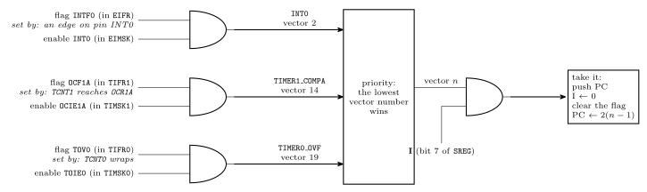
Figure 12: Whether a request becomes an interrupt, drawn as the logic it amounts to. Each source has a flag, set by its event, and an enable bit, set by the program. The source requests an interrupt only while both are 1, and all three sources here are gated the same way. If more than one is requesting, the lowest vector number wins. The winner is taken only if the I bit is also 1, and taking it clears I. For these sources, taking the vector also clears the flag. So a flag with its enable bit off simply stays set, available to be polled, and a flag that goes up while I is 0 waits and is taken the moment I returns to 1.
For the sources the course meets, the bits are:
| Source | Flag (register) | Enable (register) | Conditions set up in |
|---|---|---|---|
INT0 (pin PD2) |
INTF0 (EIFR) |
INT0 (EIMSK) |
EICRA: bits ISC01, ISC00 choose low level 00, any change 01, falling edge 10 or rising edge 11 |
TIMER0_COMPA |
OCF0A (TIFR0) |
OCIE0A (TIMSK0) |
TCCR0A, TCCR0B, OCR0A |
TIMER0_OVF |
TOV0 (TIFR0) |
TOIE0 (TIMSK0) |
TCCR0A, TCCR0B |
TIMER1_COMPA |
OCF1A (TIFR1) |
OCIE1A (TIMSK1) |
TCCR1A, TCCR1B, OCR1A |
TIMER1_OVF |
TOV1 (TIFR1) |
TOIE1 (TIMSK1) |
TCCR1A, TCCR1B |
The naming pattern is regular: an F for the flag and an IE for interrupt enable, with OC for output compare and TOV/TOIE for timer overflow. Each of these flags is cleared automatically when its vector is taken, so a handler does not normally clear its own flag. A program that polls a flag instead, with the interrupt left disabled, must clear it itself (avr-timers-and-counters).
The I bit
| I | Also | |
|---|---|---|
sei |
← 1 | |
cli |
← 0 | |
| taking an interrupt (hardware) | ← 0 | pushes PC, loads the vector address |
reti |
← 1 | pops PC |
I is bit 7 of SREG (avr-architecture), and it is 0 after reset, so no interrupt happens until the program executes sei. Because the hardware clears it on entry, a handler runs with interrupts off unless it turns them back on itself.
External interrupts
An external interrupt is requested by a pin. The ATmega324A has three, each fixed to one pin:
| Interrupt | Pin |
|---|---|
INT0 |
PD2 |
INT1 |
PD3 |
INT2 |
PB2 |
What the pin has to do to make a request is chosen by two sense control bits per interrupt, in EICRA:
ISCn1:0 |
A request is made |
|---|---|
00 |
for as long as the pin is low |
01 |
on any change of the pin |
10 |
on a falling edge, 1 to 0 |
11 |
on a rising edge, 0 to 1 |
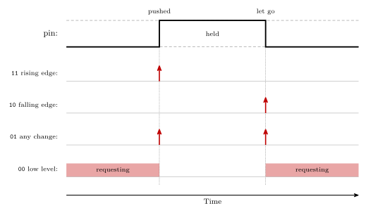
Figure 13: What each sense control setting responds to, for a push button that reads 1 while it is held. A rising edge is the moment the button is pushed and a falling edge is the moment it is let go. Any change gives a request at both. The low level setting is different in kind: it asks for the whole time the pin is low, so the handler runs again and again until the pin goes high.
Setting one up follows the same steps as any other interrupt. For a rising edge on INT0 and a falling edge on INT1:
ISR(INT0_vect) { /* PD2 went from 0 to 1 */ }
ISR(INT1_vect) { /* PD3 went from 1 to 0 */ }

/* in main */
EICRA = (1<<ISC01) | (1<<ISC00) | (1<<ISC11);   /* INT0 rising, INT1 falling */
EIMSK = (1<<INT0) | (1<<INT1);                  /* enable both               */
EIFR  = (1<<INTF0) | (1<<INTF1);                /* clear both flags          */
sei();- Edges fit buttons. An edge happens once per push, however long the button is held. That makes an external interrupt a natural way to act on a push or on a release without the program having to remember what the button was doing last time.
- Bounce. A mechanical contact chatters for a moment as it closes, and each chatter is an edge. One push can then run the handler several times.
- The low level setting keeps asking. If the pin is still low when the handler returns, the interrupt is taken again straight away.
- Priority.
INT0,INT1andINT2are vectors 2, 3 and 4, directly after reset, so they come before every timer and serial interrupt.
Used for the start/stop and reset buttons of a stopwatch in week9-lab-avr-interrupts.
Writing an ISR in assembly
The template:
isr_label:
    push r0              ; save r0: it is about to carry SREG
    in   r0, SREG
    push r0              ; save the interrupted program's flags

    ; ... perform the operation, usually input/output ...
    ; (any other register used: push it here, pop it below)

    pop  r0
    out  SREG, r0        ; flags back as they were
    pop  r0              ; r0 back as it was
    reti                 ; pop PC and set I
SREG cannot be pushed directly, because push takes a general-purpose register. So one register carries it, and that register is saved first. The restore is the save in reverse. Two consequences follow from where the save happens:
- The flags saved are the interrupted program’s. Apart from I, the hardware does not touch them on entry, and
pushchanges none, so the copy is exactly what the interrupted code left. - The saved I bit is 0, because the hardware cleared it before the first instruction of the ISR. Writing the copy back therefore leaves interrupts off until
reti, which is the right moment for them to come back.
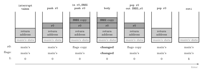
Figure 14: The stack through the ISR template, with the three things the interrupted program relies on (r0, its flags, and the I bit) traced underneath. The hardware’s push of the return address comes first, then the template’s two pushes, the SREG copy on top. The body is free to change r0 and the flags because both are safely on the stack. The restore pops the copy into r0 and writes it to SREG, then pops r0’s own value. When reti runs, the return address is on top again, exactly as the hardware left it. I stays 0 from entry to reti, the copy in the middle included, and it is reti that sets it.
Which registers to save is decided by what the body does. Save any register the body writes. Save SREG if any instruction in the body changes a flag, which rules in arithmetic, logic, compares and shifts but not in, out, ldi, mov, push or pop (avr-instructions). A handler that only copies a port to another port needs one register and no SREG at all (worked in 2026-09-21-interrupts).
Placing the entry in the table
The template in avr-program-structure puts jmp RESET at 0x0000 and leaves a comment where the handlers go. Once a vector is used, its jmp has to sit at exactly that vector’s address. The assembler’s .org directive sets the address of whatever comes next (assembly-process):
.include "m324Adef.inc"

.org 0x0000
        jmp  RESET
.org 0x001A              ; vector 14: TIMER1_COMPA
        jmp  timer1_compa_isr
.org 0x003E              ; first address after the table
RESET:
        ; stack pointer, ports, timer 1, TIMSK1 ...
        sei
loop:
        ; ...
        rjmp loop

timer1_compa_isr:
        push r0
        in   r0, SREG
        push r0
        ; ...
        pop  r0
        out  SREG, r0
        pop  r0
        reti
An assembly program that uses interrupts must also set up the stack pointer before the first sei (procedures-and-the-stack), since taking an interrupt pushes the return address.
Writing an ISR in C
#include <avr/interrupt.h>

ISR(INT0_vect) {
    /* code here */
}
ISR is a macro from avr/interrupt.h, and its argument names the vector: the source name from the datasheet followed by _vect (the table above). From it the compiler does everything the assembly programmer does by hand. The vector table is set up automatically: the handler’s jmp goes in the right entry. Registers are saved and restored automatically, SREG included, and the function ends in reti. What ISR() does not do is any of the four setup steps. In C, as in assembly, the program still sets up the conditions, enables the interrupt, clears its flag and calls sei(). sei() and cli() are macros for the single instructions.
A complete example
Timer 1 in CTC mode, matching eight times a second, with the handler toggling an LED and counting ticks. The timer set-up is Lab 12’s (week8-lab-avr-timers): \(8\,\text{MHz} / (64 \times 15625) = 8\ \text{Hz}\).
#include <avr/io.h>
#include <avr/interrupt.h>

volatile uint8_t ticks = 0;            /* written by the ISR, read by main */

ISR(TIMER1_COMPA_vect) {
    PORTA ^= (1<<0);                    /* toggle the LED on PA0 */
    ticks++;
}

int main(void) {
    DDRA = (1<<0);                      /* PA0 is an output */

    /* 1. conditions: CTC mode, clock/64, match at 15624 */
    OCR1A  = 15624;
    TCCR1A = 0;
    TCCR1B = (1<<WGM12) | (1<<CS11) | (1<<CS10);

    /* 2 and 3. clear any stale match, then enable this interrupt */
    TIFR1  = (1<<OCF1A);
    TIMSK1 = (1<<OCIE1A);

    /* 4. enable interrupts globally */
    sei();

    while (1) {
        if (ticks >= 8) {               /* a second has gone by */
            ticks = 0;
            /* ... once-a-second work ... */
        }
        /* ... anything else: the LED keeps time by itself ... */
    }
}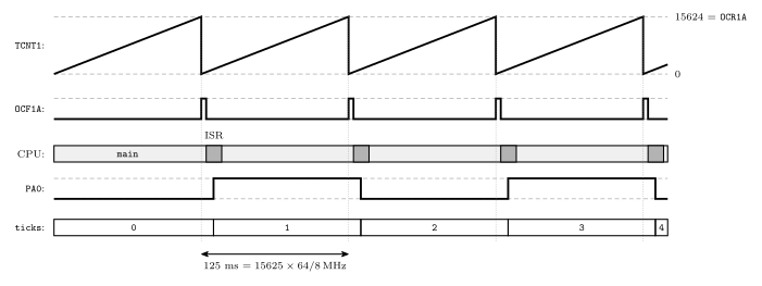
Figure 15: The example program running, one trace per signal. The count climbs to OCR1A = 15624 and is cleared (CTC mode), once every 125 ms. Each match sets OCF1A; the interrupt is enabled and I is 1, so the vector is taken a few cycles later, and taking it clears the flag again. The handler is a sliver of time in which the LED output is toggled and ticks counted, and the rest of the time belongs to main. Nothing in main looks at the timer. The LED blinks at 4 Hz, one toggle per match, however busy main is.
Priority
Priority is determined by vector: the lowest vector is the highest priority. RESET is highest, then INT0, and so on down the table. On the AVR, priority only matters when two or more interrupts are waiting to be serviced, and it decides which is taken first. It never lets one interrupt cut into another’s handler, because I is 0 throughout a handler. The datasheet adds one rule: after reti, the CPU always executes one instruction of the interrupted program before taking the next waiting interrupt, so a stream of interrupts can slow main down but never stop it altogether.
Interrupts can be re-enabled inside a handler with sei. Any incoming or waiting interrupt may then be serviced immediately, nested inside the current handler, even if it has lower priority. Priority plays no part there. Both cases are traced in 2026-09-21-interrupts and set against true priority nesting in polling-and-interrupts.
Pitfalls
- Forgetting
sei(). Everything else is set up, and nothing ever happens, because I is 0 from reset. - Enabling an interrupt that has no handler. In C, avr-libc fills every unused vector with a jump to a default handler that jumps to address 0, so the program restarts whenever the event occurs. It is not a true reset: the I/O registers keep whatever they held, which can make the restart behave differently from a power-up.
- Misspelling the vector name.
ISR(TIMER1_COMPA_Vect)compiles with only a warning, and the handler is never placed in the table, which makes it the previous pitfall. - Not clearing a stale flag before enabling: the interrupt fires once immediately, for an event that happened before the program was ready.
- Clearing a flag with
|=. If the compiler turns it into a read, an OR and a write, it clears every flag in the register that happens to be set (avr-timers-and-counters). Writing just the one bit,TIFR1 = (1<<OCF1A);, is safe however it is compiled. - In assembly: not saving
SREG, unbalanced pushes and pops, orretinstead ofreti. The first corrupts the interrupted code’s flags. The second returns to the wrong address. The third returns correctly but leaves I at 0, so no interrupt ever happens again. - Long handlers. No delay loops and no waiting inside an ISR: every other interrupt waits too, and repeated events of one source merge into one.
- A shared variable without
volatile, or a multi-byte one read withoutcli().
See also
- polling-and-interrupts — polling versus interrupts, the fourteen-step sequence, transparency, nesting policies, traps
- 2026-09-21-interrupts — Lecture 17: the stack revisited, worked questions,
volatiledrawn, priority traced - avr-timers-and-counters — the timer interrupt registers
TIMSKnandTIFRn, and the flags these interrupts replace polling - procedures-and-the-stack — the stack the return address goes on, and initialising
SP - avr-program-structure — the
jmp RESETtemplate the vector table extends - avr-architecture —
SREGand its I bit · avr-instructions — which instructions change the flags - c-preprocessor-and-avr-headers —
volatilein the I/O register macros · bit-masking —(1<<OCIE1A) - week8-lab-avr-timers — Lab 12, the timer set-up the example uses
- week9-lab-avr-interrupts — Lab 14: a stopwatch from a timer interrupt and two external interrupts
- software-timers — one timer interrupt keeping time for the whole program
- avr-usart — the three serial interrupts · analog-to-digital-conversion — the conversion-complete interrupt · avr-spi — the transfer-complete interrupt
C Language Basics
What a C program is made of: the shape of a program, variables and their types, functions, and constants. Operators are in c-operators, the if/while/for statements in c-control-flow, arrays and pointers in c-pointers-and-arrays, and the preprocessor in c-preprocessor-and-avr-headers. First met in 2026-09-07-introduction-to-embedded-c-programming.
Where C sits
C is the top layer of the course’s three blocks — high-level programming over low-level programming over digital logic design — and the course’s C is embedded C for the ATmega324A, the same chip the assembly targeted. The difference from assembly is one extra tool. An assembler turns each line into exactly one instruction; a compiler turns each C statement into however many instructions it needs, chooses the registers, and hands the result to the assembler. The chain from C statement down to control unit is drawn in 2026-09-07-introduction-to-embedded-c-programming, and the steps after the compiler, object files and the linker, are in compilation-and-linking.
What is expected: write small C programs and functions from scratch, understand the meaning of C programs, and write or modify C programs — practised in Labs 11–16, which all use C.
The shape of a program
- There must be a function called
main; it is executed when the program starts. - Blocks of code are enclosed by braces
{ }. - Statements end with a semicolon
;. - C is case sensitive —
variableandVariableare different names. - Comments are
/* … */(any length, may span lines) or//to the end of the line.
/* the smallest useful embedded program: */
#include <avr/io.h>

int main(void) {
    DDRA = 0xFF;        /* a statement */
    while(1) {          /* a block */
        PORTA = 0x55;
    }
}
On the AVR main never returns — there is no operating system to return to — so every program ends in an infinite loop (c-control-flow). #include is the preprocessor’s (c-preprocessor-and-avr-headers).
Variables and types
Declaration: type-name variable-name, variable-name …;
A declaration reserves room in data memory (memory-models) and gives it a name and a type. The type decides two things: how many cells the variable takes, and how the bits are read — the signed/unsigned question of binary-number-representations, now answered once at the declaration instead of instruction by instruction.
| Declaration | Size | Range | |
|---|---|---|---|
char c; |
1 byte | −128 … 127 | two’s complement |
unsigned char x; |
1 byte | 0 … 255 | |
int day; |
machine dependent — 16 bits on the AVR | −32768 … 32767 | two’s complement |
unsigned int count; |
as int |
0 … 65535 on the AVR | |
float |
32 bits | about \(\pm 3.4 \times 10^{38}\), 7 digits | IEEE single precision; no AVR hardware — done in software |
double |
64 bits in general; 32 on avr-gcc | likewise |
On avr-gcc float and double are interchangeable: both are 32 bits (below).
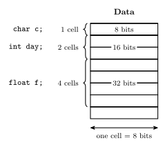
Figure 16: What three declarations reserve in the AVR’s 8-bit data memory, drawn as a memory map. char is one cell. int is two, because int is 16 bits on the AVR — which is why a pointer to an int steps by two in the pointers note. float is four, because single precision is 32 bits. The compiler decides the actual addresses; the addresses here are schematic and the order is arbitrary.
Three consequences worth carrying around:
charis an integer. It is exactly the 8-bit two’s complement byte of the hardware block; the name only promises it can hold a character code. Arithmetic on it is byte arithmetic, and'A' + 1is'B'because'A'is 65.intis not one size. Write code that assumes 16 bits and it breaks on a desktop; assume 32 and it breaks on the AVR. The AVR headers provideuint8_t,int16_tand friends — types with the width in the name — and the course’s example program usesuint8_tfor exactly this reason.- Nothing is checked. Storing 300 in an
unsigned chardoes not fail; it stores 300 mod 256, i.e. 44. (For a signedcharthe C standard leaves the result implementation-defined; gcc also gives 44.) The type is a reading rule, not a guard.
Booleans. There is no boolean type in the course’s C. Any value can be treated as a boolean: zero means false, non-zero means true. This is what lets if(a) mean if(a != 0) (c-control-flow).
Functions
return-type function-name (arg-decl)
{
    variable-declarations;
    …
    statements;
}| Part | Meaning | Example |
|---|---|---|
return-type |
what type is returned, or void for nothing |
int, void |
function-name |
the name; main for the entry point |
average |
arg-decl |
argument (parameter) declarations, comma-separated, each with its type | int a, float b |
variable-declarations |
variables used only within the function | int avge; |
statements |
the code which actually does stuff |
An example:
/*
  Return the average of two integers
  (result will be rounded towards 0)
*/
int average(int a, int b) {
    int avge;

    avge = (a+b)/2;

    return avge;
}
avge = (a+b)/2;is a statement built from expressions —(a+b), then(a+b)/2, then the assignment; the outermost expression plus its semicolon is the statement.return avge;hands the value back and ends the function.avgeis local: it exists only whileaverageis running. Nothing outside can name it.- Integer division truncates toward zero.
average(1, 2)computes3/2and returns1; the.5never exists. The comment says rounded towards 0, and that is the whole of C’s rule for/on integers —-3/2is-1, not-2.
A function with void in front returns nothing and is called for its effect. int main(void) is a function whose argument list is explicitly empty.
Where a variable lives
Where a declaration is written decides where the compiler stores the variable and how long it exists.
| Declaration | Kind | Stored | Exists |
|---|---|---|---|
outside every function: int count; |
global | at a fixed address in data memory, from 0x0100 up |
for the whole run |
inside a function: int avge; |
local | in the call’s stack frame | only while that call runs |
inside a function: static int calls; |
static local |
with the globals, at a fixed address | for the whole run, keeping its value between calls |
outside every function: static int a; |
static global |
like any global | for the whole run; the name is private to its file |
So avge in average above is made fresh on every call and is gone at the return, and a local that is never assigned starts out holding whatever was left on the stack. A static local is the way to have a function remember something from one call to the next. Memory obtained from malloc() comes from a third place, the heap, which grows from above the globals toward the stack. The full picture is in compilation-and-linking, and the frame itself is in procedures-and-the-stack.
Constants
Character constants
Single quotes: 'a', 'b', '1'. A character constant is a number — its ASCII code — so '1' is 49, not 1.
| Range | Codes |
|---|---|
'A' … 'Z' |
65 … 90 |
'a' … 'z' |
97 … 122 |
'0' … '9' |
48 … 57 |
Which makes c - '0' the digit value of a digit character, and c + ('a' - 'A') the lower-case of an upper-case letter — both plain integer arithmetic.
Special characters are backslash escaped:
'\n' |
newline |
'\'' |
single quote |
'\t' |
tab |
'\\' |
backslash |
String constants
Double quotes, escapes allowed inside: "abc \n \" hello\t". A string is an array of char (c-pointers-and-arrays).
Integer constants
| Base | Written | Examples |
|---|---|---|
| Decimal | as usual | 3, -27, 65535, +5 |
| Hexadecimal | leading 0x |
0x5F, 0xFFFF, 0xDEADBEEF |
| Octal | leading 0 |
0377 = 255 |
The octal rule is a trap: a leading zero changes the base. 010 is eight. Do not zero-pad a decimal constant.
Hexadecimal is the natural notation for anything that is really a bit pattern — port values, masks — because each digit is exactly one nibble (binary-number-representations). 0xFF is 11111111 at a glance; 255 is not.
Floating point constants
Include a decimal point and/or an e exponent: 3.1416, -7., 6.02e23, -5.2e-2. 7 is an integer; 7. is floating point. The type of a constant is decided by how it is written, and it decides what arithmetic happens: 7/2 is 3, 7./2 is 3.5.
Floating point on the AVR
float and double are usually IEEE single and double precision, but the C standard only asks for minimums: about 6 significant decimal digits for float and 10 for double, both up to \(10^{37}\). avr-gcc makes double the same 32-bit single precision as float, which gives about 7 digits and so falls short of what the standard asks of double. Code written for a desktop that relies on double quietly loses half its digits on the AVR.
The AVR also has no floating-point hardware: its only hardware data type is the 8-bit integer (instruction-set-architecture). Every float add, multiply or conversion is a call into a software library, hundreds of instructions with branches where an integer operation takes a few. So where integer arithmetic can give the same result, use it:
PORTB = PINA / 3;        /* integer: a handful of instructions, no branches */
PORTB = PINA * 0.334f;   /* float: the same results, 300+ instructions      */
Scaling to whole units (millivolts, tenths of a degree) or using fixed-point-numbers keeps the fractions without the floats. The formats themselves, and why 0.1 cannot be stored exactly, are in floating-point-numbers.
See also
- c-operators · c-control-flow · c-pointers-and-arrays · c-preprocessor-and-avr-headers
- binary-number-representations — the signed/unsigned readings behind
charandunsigned char - floating-point-numbers — what
floatanddoublehold, and their cost on the AVR · fixed-point-numbers — fractions in integer arithmetic - memory-models — the 8-bit data cells a declaration reserves
- instruction-set-architecture — the data types the AVR supports in hardware, and the ones it does not
- compilation-and-linking — how the compiler maps globals, locals and statics to memory, and what happens after compiling · procedures-and-the-stack — the stack frame a local lives in
- 2026-09-07-introduction-to-embedded-c-programming — Lecture 13 · 2026-10-15-compilation-and-linking — Lecture 22 · 2026-10-19-floating-point-numbers — Lecture 23
C Preprocessor and AVR Headers
The preprocessor — #include and #define — and the three lines of avr/io.h that let DDRA = 0xFF; be written as if a hardware register were a variable. First met in 2026-09-10-more-c-programming-on-the-avr; the port registers themselves are in avr-io-ports.
What the preprocessor is
C programs are first parsed by a preprocessor, which replaces preprocessor directives with substitute text. Only then does the compiler see the program. Directives start with #:
| Directive | Does |
|---|---|
#include … |
paste in a file |
#define … |
define a macro — a textual substitution |
#if, #ifdef, #else, #undef, … |
conditional inclusion, un-definition, and others |
The preprocessor does not know C. It edits text. Whatever it produces is what the compiler compiles, and every surprise in this note comes from forgetting that.
#include
| Form | Kind of header | Looks in |
|---|---|---|
#include <filename.h> |
system | the system include directories — where avr/io.h and stdio.h live |
#include "filename.h" |
user-defined | your own project directory first |
The directive is replaced by the whole contents of the named file, at that point. After preprocessing there is one file, with the header pasted in at the top.
Header files
Header (.h) files are used for common macros, function prototypes etc — the C counterpart of m324Adef.inc in assembly (avr-io-ports).
stdio.h— prototypes ofprintf()etc. The AVR has a simplified version (no files);printf()only works if you say where the characters go, e.g. a serial port.avr/io.h— defines the AVR’s useful constants and functions/macros. Definitions depend on the actual device targeted: it reads which chip is being compiled for and pulls in that chip’s register map, soDDRAmeans the right address for the ATmega324A and a different one for another part. It also suppliesuint8_tand the other fixed-width types.
Every program in the course starts with #include <avr/io.h>.
Headers against libraries
A header file is not the library. A header
- defines useful preprocessor macros,
- declares the functions that are in the library, as function prototypes, and
- declares variables that are available externally, with
extern.
The library is the collection of object files that implements the functions (compilation-and-linking).
A prototype such as int printf(const char *fmt, ...); tells the compiler the name, the argument types and the return type. That is enough for the compiler to check a call and generate it. There is no code in it, so in main.o the call to printf is left as an external reference. The code is in the library, an object file printf.o inside it, and the linker joins it on and fills in the address. An extern declaration does the same for a variable: extern int count; says that count exists somewhere else and reserves nothing.
So the header goes to the compiler, through the preprocessor, and the library goes to the linker. The two kinds of mistake show up at different steps:
| Missing | Shows up when | Typical message |
|---|---|---|
the #include |
compiling | implicit declaration of function printf |
the library, or the .c file that defines the function |
linking | undefined reference to printf |
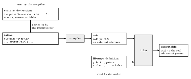
Figure 17: Where a header and a library each come into play, for a program that calls printf. The header holds only declarations. The preprocessor pastes it into main.c so that the compiler can check and generate the call, and in main.o that call is still an external reference. The library holds the definitions, as already compiled object files with an index. The linker finds printf.o through the index, links it in, and fills in the call. The header is used by the compiler and the library by the linker.
#define — macros
Macros are textual substitutions.
| Macro | Effect |
|---|---|
#define pi 3.1415 |
every later pi becomes 3.1415 — A = pi * r²; becomes A = 3.1415 * r²; (the superscript is shorthand; in real C the square would be r * r) |
#define EVER ;; |
for(EVER) becomes for(;;), an infinite loop |
#define sum(a,b) (a+b) |
a macro with parameters: sum(x, 2) becomes (x+2) |
A macro with parameters looks like a function call and is not one: no call happens, the arguments are pasted into the body as text, and the result is compiled in place.
The SQUARE trap
Given
#define SQUARE(x) (x*x), what isSQUARE(1+2)?
5, not 9. Paste the text: (1+2*1+2). Multiplication binds tighter than addition, so it is \(1 + 2 + 2\). The argument was never evaluated first, because there is no function to evaluate it.
The fix is parentheses around every parameter, and around the whole body:
#define SQUARE(x) ((x)*(x)) /* SQUARE(1+2) -> ((1+2)*(1+2)) = 9 */The outer pair matters as much as the inner: without it, 1 / SQUARE(a) becomes 1 / (a)*(a), which is \(a\), not \(1/a^2\). Write every macro this way. The AVR headers below do — note the brackets around (mem_addr) and (io_addr).
A second pitfall: an argument with a side effect is pasted as many times as the parameter appears. SQUARE(i++) becomes ((i++)*(i++)) and increments i twice.
The avr/io.h register macros
The definitions behind the port names, from avr/io.h and the device header it includes:
#define _MMIO_BYTE(mem_addr) \
                (*(volatile uint8_t *)(mem_addr))
#define _SFR_IO8(io_addr) \
                _MMIO_BYTE((io_addr) + 0x20)

/* Input Pins, Port A */
#define PINA      _SFR_IO8(0x00)

/* Data Direction Register, Port A */
#define DDRA      _SFR_IO8(0x01)

/* Data Register, Port A */
#define PORTA _SFR_IO8(0x02)(\ at the end of a line continues a directive onto the next line.)
Upshot: I/O register names can be used as variables.
DDRA = 0xFF;
PORTA = PINC | 0xF0;
Unrolling DDRA
| Step | Text |
|---|---|
| as written | DDRA = 0xFF; |
#define DDRA |
_SFR_IO8(0x01) = 0xFF; |
#define _SFR_IO8 |
_MMIO_BYTE((0x01) + 0x20) = 0xFF; |
#define _MMIO_BYTE |
(*(volatile uint8_t *)((0x01) + 0x20)) = 0xFF; |
Reading the final line from the inside out:
(0x01) + 0x20is0x21— a number.(volatile uint8_t *)casts it: treat this number as the address of an 8-bit unsigned byte. Now it is a pointer (c-pointers-and-arrays).- The leading
*dereferences it: the byte at that address. = 0xFFstores into that byte.
So DDRA = 0xFF; is a store to data address 0x21, and x = PINC; is a load from data address 0x26. There is no variable called DDRA anywhere; the name dissolves before the compiler sees it.
Why + 0x20
The AVR’s 64 I/O registers have two addresses each (avr-io-ports): an I/O-space number 0–63, which is what in and out use, and a data-space address 0x20 higher, where lds/sts — and any C pointer — find the same register. DDRA is I/O 0x01 and data 0x21. The macro takes the I/O number the datasheet lists and adds the offset, because a C pointer can only name data-space addresses. (The compiler, seeing a constant address in the I/O range, will usually emit in/out anyway.)
Why volatile
volatile tells the compiler the value at this address can change without the program changing it, and that every read and write matters. Without it the compiler is entitled to assume that a byte it wrote a moment ago still holds what it wrote, and that two reads with nothing between them give the same answer — both false for a port: PINC changes whenever the pins do, and PORTA is written for its effect on the pins, not to be read back. volatile forbids the optimisations that would break that. It is the one piece of the macro that is about hardware rather than addressing.
The same keyword belongs on any ordinary variable that an interrupt handler writes. To the code in main, a handler’s write is as invisible as a pin changing, and for the same reason: nothing in main’s own flow of control explains it. See avr-interrupts.
Naming bits
The headers also define bit numbers for every flag and pin — for example FLAG_NAME == 5 — so a mask is written from a name rather than a constant:
1 << FLAG_NAME              /* 00100000 when FLAG_NAME is 5 */
PORTA |= (1 << 5);          /* set one bit                   */
PORTA &= ~(1 << 5);         /* clear one bit                 */
The shift and the |=/&= shorthands are in c-operators; the mask patterns are in bit-masking. FLAG_NAME is a placeholder name; the actual names for the ATmega324A’s pins and flags come from the device header, as #define WGM02 3 does in 2026-10-05-more-io.
See also
- avr-io-ports — the port registers, and the I/O-space versus data-space address columns
- c-pointers-and-arrays — what
*(uint8_t *)addrmeans - c-operators —
1 << n,|=,&= - bit-masking · memory-models
- avr-interrupts —
volatileon variables shared with an interrupt handler - compilation-and-linking — what happens after the preprocessor: object files, libraries and the linker · 2026-10-15-compilation-and-linking — Lecture 22
- 2026-09-10-more-c-programming-on-the-avr — Lecture 14
Compilation and Linking
How a C program turns into the machine code in the AVR’s flash. This note covers compiling against interpreting, where the compiler puts global, local and static variables, object files and their six sections, the linker’s two jobs (relocating and resolving), libraries, how header files differ from libraries, and static against dynamic linking. The assembler’s part, with its two passes and symbol table, is in assembly-process. First met in 2026-10-15-compilation-and-linking.
Compiled or interpreted
A processor runs machine code and nothing else. The fetch-decode-execute cycle (fetch-decode-execute-cycle) reads instruction words from memory, and nothing in it knows the program was once written in C. A program in a high-level language reaches the processor in one of two ways.
- Compilation translates the whole program into machine code before it runs, often by way of assembly language. The machine code then runs directly on the processor. C works this way.
- Interpretation never turns the program into machine code. Another program, the interpreter, reads the source and carries out each statement when it gets to it. The interpreter is itself machine code, and it is the interpreter that the processor runs. Python, Java and MATLAB work this way.
| Compiled | Interpreted | |
|---|---|---|
| What the processor runs | the program’s own machine code | the interpreter’s machine code |
| When translation happens | once, before the program runs | every time a statement is executed |
| Speed | fast | slow |
| Portability | the machine code suits one processor only | runs anywhere an interpreter exists |
Why interpreting is slow. Every time a statement is executed, the interpreter has to work out again what the statement means and then carry it out. That costs many of its own instructions per statement, and inside a loop it is repeated on every pass. A compiler does that work once, ahead of time.
Why it is portable. The program never becomes machine code, so nothing in it is tied to one instruction set. Moving it to a new processor only needs an interpreter built for that processor.
Bytecode and just-in-time compilation
Java and Python take a route in between. The source is first compiled, but not into machine code. It becomes bytecode, the instruction set of an imaginary machine. Bytecode is the same on every platform, so a compiled Java program is portable across all of them.
The bytecode is then run by a virtual machine, which is an interpreter for bytecode. The Java Virtual Machine is the one for Java. Running bytecode is faster than interpreting source text, because the parsing has already been done, but it is still interpretation.
To win back the speed, the virtual machine watches which parts of the program run most often and compiles them into real machine code while the program is running. This is just-in-time (JIT) compilation. Once a part has been JIT-compiled, it runs directly on the processor like compiled code. Standard Python interprets its bytecode, and a JIT compiler such as Numba can compile chosen Python functions to machine code in the same way.
The toolchain
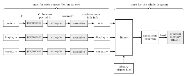
Figure 18: How a three-file C program becomes a running program. Each source file goes through the first three steps by itself. The preprocessor pastes in headers and expands macros, the compiler turns C into assembly, and the assembler turns assembly into an object file, which is machine code plus the information needed to link it. Only the linker sees the whole program. It joins the object files to each other and to the library members they use, fixes up every address, and writes one executable. That executable is then loaded into memory, which on the AVR means programming it into flash. Changing one source file means repeating the first three steps for that file alone, then linking again.
| Step | Takes | Produces | Notes |
|---|---|---|---|
| Preprocess | a .c file |
C with every #include pasted in and every macro expanded |
c-preprocessor-and-avr-headers |
| Compile | that C | assembly language | maps variables to memory, and translates each statement into instructions |
| Assemble | the assembly | an object file, .o |
assembly-process |
| Link | all the object files, plus the library | one executable | relocates and resolves addresses |
| Load | the executable | the program in memory, ready to run | on the AVR, the executable is programmed into flash |
Some compilers write machine code directly and never produce assembly text. The object file that comes out is the same either way, so the three middle steps are often just called “compiling”. In the simplified view the compiler itself does two things, mapping variables to memory and translating C into assembler instructions. Turning those instructions into machine code is the assembler’s work.
With the AVR GCC toolchain the object files and the executable are ELF files. The .hex file that gets programmed into flash is extracted from the ELF executable.
How a compiler maps variables to memory
The compiler decides where each variable goes by how long it has to exist.
| Declared | Lives | Stored | Address |
|---|---|---|---|
| outside every function: a global | for the whole run | in the fixed data area, which starts at the bottom of SRAM | fixed before the program runs |
| inside a function: a local | only while that call is running | in the call’s stack frame | depends on how deep the stack is at the call |
inside a function, marked static |
for the whole run, and it keeps its value between calls | with the globals | fixed |
nowhere: obtained from malloc() |
until it is given back | on the heap | handed out while the program runs |
Globals. A global can be used at any moment from any function, so it needs one address that never changes. The compiler reserves as many bytes as the type needs (c-language-basics), one variable after another, from the start of SRAM. On the ATmega324A that is 0x0100 = 256, because addresses 0 to 255 are taken by the registers and the I/O registers (memory-models). It is the same thing an assembly programmer does with .dseg and .byte.
Locals. A local exists only while its function is running, and a recursive function can have several calls running at once, each needing its own copy. So the compiler cannot give it a fixed address. Instead, each call builds a stack frame, a block on the stack holding that call’s arguments, its return address and its local variables. The return takes the frame away again (procedures-and-the-stack). The same local therefore sits at different addresses on different calls.
static locals. static inside a function keeps the name private to the function but gives the variable a global’s lifetime. It is stored with the globals, at a fixed address, and is never part of a frame. That is why it still holds its value the next time the function is called.
static on a global means something else. The variable is stored exactly like any global, but its name is private to its own source file. It is left out of the object file’s entry point table (below), so no other file can link to it.
The heap and the stack grow toward each other. The heap starts above the globals and grows toward higher addresses. The stack starts at the top of SRAM (RAMEND) and grows down. The free memory between them shrinks from both ends, and if the two meet, that is a stack overflow. Nothing on the chip detects it. The first sign is usually a global or heap variable changing for no reason.
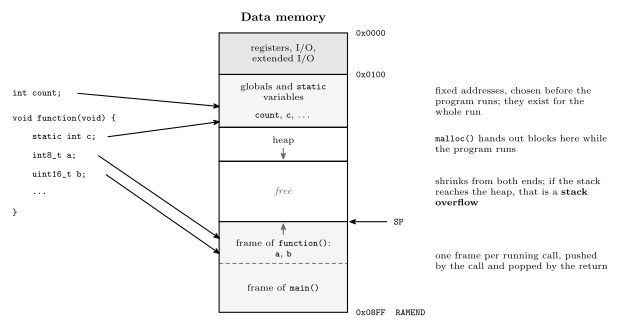
Figure 19: Where each kind of C variable ends up in the ATmega324A’s data memory, with the lowest address at the top. Globals and static variables are given fixed addresses from 0x0100, the first SRAM byte, so a static local such as c sits among the globals even though only its own function can name it. The heap, which malloc() hands out while the program runs, grows down the page toward the stack. The stack grows up the page from RAMEND. Each running call has a frame on it, and the frame of function() holds its locals a and b. When function() returns, that frame is gone. If the stack and the heap meet, the stack has overflowed.
Object files
A program of any size is split into several source files, and it pays to compile or assemble each one separately and then link them together. Change one file and only that file has to be compiled again. The others’ object files are reused as they are.
The price is that when a file is compiled, nobody knows where its code will end up. The file is translated as if it started at address 0. Every address inside it is relative to its own start, and any symbol defined in another file has no address at all yet. Once the linker has decided where everything goes, these addresses have to be fixed. A file that carries enough information for that fixing is a relocatable object module. “Object module” and “object file” mean the same thing.
So an object file is machine code plus information for the linker. There are many formats for it: a.out, COFF and ELF are object file formats, and DWARF is a format for debugging information, usually carried inside ELF files.
The six sections
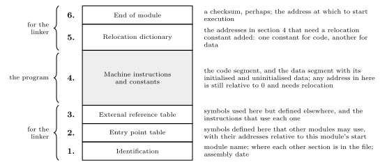
Figure 20: The six sections of a relocatable object module, numbered from the bottom. Only section 4 is program: the machine instructions and constants, assembled as if the module began at address 0. The other five are information for the linker. They say what the module is called and where its parts are in the file (1), which of its symbols other modules may use (2), which symbols it uses but does not define (3), which addresses in section 4 have to be moved when the module is moved (5), and where execution starts (6). Linking reads 1, 2, 3, 5 and 6 to decide how to rewrite 4.
1. Identification. The name of the module, where each of the other sections is in the file, and the date it was assembled.
2. Entry point table. The symbols defined in this module that other modules may refer to, with their values. A value is an address: a procedure’s entry point, or a variable’s location. It is relative to the beginning of this object module. A file that defines a procedure abs_value at its address 10 has the entry abs_value 10. Anything not listed, such as a static global or a label used only inside the module, cannot be reached from another file.
3. External reference table. The symbols used in this module but not defined in it, both procedure names and variables, and for each one the list of instructions that use it. Those instructions are the places the linker will have to fill in once it knows the address.
One module’s entry point is another module’s external reference. If module A defines SUM and module B calls it, SUM appears in A’s entry point table and in B’s external reference table.
4. Machine instructions and constants. The assembled code and constants: the code segment, and the data segment holding the initialised and the uninitialised data. An initialised global such as int n = 5; needs its starting value stored in the file. An uninitialised one needs only its size. The addresses used in this code are not yet correct. They were worked out as if the module started at 0, so they need relocation.
5. Relocation dictionary. The list of addresses in section 4 that need to be relocated. When the module is placed, a relocation constant is added to the instruction or data at each of those addresses. There is one constant for code and a different one for data, because a module’s code goes in program memory and its data in data memory, and the two start in different places.
6. End of module. Possibly a checksum, to catch a corrupted file, and the address at which execution starts.
The linker
The linker combines object modules, the program’s own and any it needs from libraries, into a single executable binary program of machine code.
Its problem is the assembler’s problem again, one level up. That is the external reference problem: symbols are used before their values are known. Module A can call a procedure in module B before the linker has even read B. So the linker, like the assembler, works in two passes (assembly-process).
Pass 1: lay the program out.
- Read each module’s sizes and give it a place, in link order. Each module’s code starts where the previous module’s code ended, and the same goes for data. These starting addresses are the module’s two relocation constants.
- Read every entry point table. Add each symbol to one global symbol table, with its final address: its value relative to its module, plus that module’s starting address.
Pass 2: copy and patch.
- Copy each module’s section 4 to its place.
- Relocate. For each address in the module’s relocation dictionary, add the module’s constant, the code constant for a code address and the data constant for a data address.
- Resolve. For each external reference, look the symbol up in the global table and write its final address into every instruction listed against it. A symbol that no module defines cannot be resolved, so linking fails with an “undefined reference” error.
The two words to keep straight:
Relocating = adding a constant: fixing an address that points into the module’s own code or data, which moved when the module moved. Resolving = finding the value of an external address: filling in an address that points into another module.
Where a module starts follows from the order alone. A module’s code starts at the program start plus the code sizes of every module linked before it, and its data starts at the data start plus the data sizes of those same modules. Code and data are counted separately, in their own units: on the AVR, words of program memory and bytes of data memory (memory-models).
Worked: linking four modules
Four object modules, each assembled from address 0. Their lengths are A = 400, B = 600, C = 500, D = 300. Each holds a branch within itself, a data move, and (apart from D) a call to the next module.
| Module | At | Instruction |
|---|---|---|
| A | 0 | BRANCH TO 200 |
| A | 200 | MOVE P TO X |
| A | 300 | CALL B |
| B | 0 | BRANCH TO 300 |
| B | 300 | MOVE Q TO X |
| B | 500 | CALL C |
| C | 0 | BRANCH TO 200 |
| C | 200 | MOVE R TO X |
| C | 400 | CALL D |
| D | 0 | BRANCH TO 200 |
| D | 200 | MOVE S TO X |
They are linked in the order A, B, C, D. The first 100 addresses hold start-up code, the code that runs before main (on the AVR it sets the stack pointer and prepares the data), so A starts at 100.
Pass 1: place the modules. Each starts where the previous one ends.
| Module | Length | Starts at | Ends at | Relocation constant |
|---|---|---|---|---|
| A | 400 | 100 | 499 | +100 |
| B | 600 | 100 + 400 = 500 | 1099 | +500 |
| C | 500 | 500 + 600 = 1100 | 1599 | +1100 |
| D | 300 | 1100 + 500 = 1600 | 1899 | +1600 |
The global symbol table holds the module names as entry points: A = 100, B = 500, C = 1100, D = 1600. The program ends at 1899, and 1900 is the first free address.
Pass 2: patch each instruction. An instruction moves to its offset plus its module’s start. A branch inside a module is relocated: the target moves by the same constant as the instruction, so it still lands on the same MOVE. A call to another module is resolved from the symbol table.
| New address | Was | Becomes | Because |
|---|---|---|---|
| 100 | A: BRANCH TO 200 |
BRANCH TO 300 |
relocate: 200 + 100 |
| 300 | A: MOVE P TO X |
MOVE P TO X |
no code address in it |
| 400 | A: CALL B |
CALL 500 |
resolve: B starts at 500 |
| 500 | B: BRANCH TO 300 |
BRANCH TO 800 |
relocate: 300 + 500 |
| 800 | B: MOVE Q TO X |
MOVE Q TO X |
no code address in it |
| 1000 | B: CALL C |
CALL 1100 |
resolve: C starts at 1100 |
| 1100 | C: BRANCH TO 200 |
BRANCH TO 1300 |
relocate: 200 + 1100 |
| 1300 | C: MOVE R TO X |
MOVE R TO X |
no code address in it |
| 1500 | C: CALL D |
CALL 1600 |
resolve: D starts at 1600 |
| 1600 | D: BRANCH TO 200 |
BRANCH TO 1800 |
relocate: 200 + 1600 |
| 1800 | D: MOVE S TO X |
MOVE S TO X |
no code address in it |
B’s constant, 500, is the start-up code plus all of A: 100 + 400. Every branch ends up pointing at the instruction it pointed at before: A’s branch at 100 reaches A’s MOVE at 300, and B’s at 500 reaches B’s MOVE at 800. The MOVEs name data, P, Q, R, S and X. Those addresses are fixed in the same way with each module’s data constant, which this example leaves out so that only the code is followed.
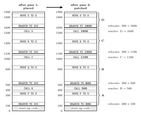
Figure 21: Linking four object modules in the order A, B, C, D, with addresses increasing up the page and start-up code in 0 to 99. Left: after the first pass. Every module has its place, each starting where the one before it ends, but the instructions are still exactly as assembled. A’s branch at 100 still names 200, its target counted from A’s own 0, and 200 is now in the middle of A, not at its MOVE. Each call still names a module, not an address. Right: after the second pass. Each branch within a module has been relocated by its module’s starting address, so it lands on that module’s MOVE again, and each call to another module has been resolved to that module’s start. The bold operands are the ones the linker rewrote.
Worked: where each module starts
Three modules have these sizes. Code is measured in words, because AVR program memory holds 16-bit words, and data in bytes.
| Module | Code size (words) | Data size (bytes) |
|---|---|---|
| 1 | 45 | 17 |
| 2 | 67 | 5 |
| 3 | 100 | 25 |
They are linked in the order 2, 1, 3, starting at program address 62 and data address 256. Where does each module’s code and data start, and where do two sample references inside module 1 end up?
Lay them out in link order, keeping a running total for each memory:
| Module | Code | Data | Code constant | Data constant |
|---|---|---|---|---|
| 2 | 62 to 62 + 67 − 1 = 128 | 256 to 256 + 5 − 1 = 260 | +62 | +256 |
| 1 | 129 to 129 + 45 − 1 = 173 | 261 to 261 + 17 − 1 = 277 | +129 | +261 |
| 3 | 174 to 174 + 100 − 1 = 273 | 278 to 278 + 25 − 1 = 302 | +174 | +278 |
The next free code word is 274 and the next free data byte is 303. Both totals come out the same as for any other order, because the same three sizes are added up. Only where each module falls changes.
Relocate inside module 1. Suppose module 1 has, at its own word 20, a branch to its own word 40, and at its own word 30, a load from its own data byte 4.
- The branch moves to 20 + 129 = 149, and its target is relocated by the same code constant, 40 + 129 = 169.
- The load moves to 30 + 129 = 159, and its operand is a data address, relocated by the data constant: 4 + 261 = 265.
Adding the code constant to the data address would give 133, and the load would read the wrong byte. This is why the relocation dictionary has to say whether each entry is a code address or a data address.
Why 62 and 256? On the ATmega324A, program words 0 to 61 (0x0000 to 0x003D) are the interrupt vector table (avr-interrupts), so 0x003E = 62 is the first free word. Data addresses 0 to 255 are registers and I/O, so 0x0100 = 256 is the first byte of SRAM.
Libraries
A library is a collection of object files with an additional index. It provides useful functions and procedures that have already been written, tested and compiled. The rule is not to reinvent the wheel: use library code where it exists.
The index maps each symbol to the member object file that defines it. When an external reference is still unresolved, say a call to printf, the linker looks the name up in the index, takes that one member, and links it in like any other module. The rest of the library stays out of the program.
The standard C library is the one every C program can count on. It covers:
- standard input and output (
stdio.h:printf,getchar, …) - string handling (
string.h:strlen,strcpy, …) - date and time functions (
time.h) - general utilities (
stdlib.h:malloc,abs,atoi, …)
On the AVR it is provided by avr-libc, which also supplies the avr/io.h and avr/interrupt.h headers.
Header files are not the library
The two are easy to mix up, because #include <stdio.h> is what lets a program call printf.
A header file (.h)
- defines useful preprocessor macros,
- declares the functions that are in the library, as function prototypes, and
- declares variables that are available externally, with
extern.
The library is the collection of object files that implement those functions.
A declaration says what a name is and what type it has, so the compiler can check every use and generate the call. It contains no code, so the call still has nowhere to go. The header is therefore read by the compiler, and the library is read by the linker. Each kind of mistake shows up at its own step:
| Missing | When it shows | Typical message |
|---|---|---|
| the header | compiling | implicit declaration of function printf |
| the library, or the file that defines the function | linking | undefined reference to printf |
How a header gets pasted in is covered in c-preprocessor-and-avr-headers.
Static and dynamic linking
Everything so far is static linking. All the object code, the library’s and the main program’s, is joined into one binary before the program ever runs.
In dynamic linking, linking happens at run time instead: a library procedure is linked when it is first called. The executable holds only a reference to it, and the library stays in a separate file that is loaded when the program needs it. DLLs (dynamic-link libraries) on Windows work this way, and so do shared libraries (.so files) on Linux.
| Static | Dynamic | |
|---|---|---|
| Library code is joined in | when the program is linked | when the procedure is first called |
| Library code is stored | inside every executable that uses it | once, in its own file, shared |
| Executable size | larger | smaller |
| Updating the library | means relinking each program | takes effect in every program at once |
Its advantages:
- It saves space. Libraries are not linked into the executable, so ten programs that use the same library share one copy of it.
- The library can be updated independently of the programs that use it. A bug fixed in the DLL is fixed in all of them, without relinking anything.
The second advantage is also its weakness. A program tested with one version of a library can break when another installation replaces that library with a version that behaves differently. On earlier versions of Windows this was common enough to be called “DLL hell”.
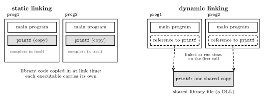
Figure 22: The same two programs, both calling printf, linked statically and dynamically. Static linking copies printf’s object code into each executable when it is linked, so each program carries its own copy and is complete in itself. Dynamic linking leaves a reference in each executable and keeps a single copy of printf in a shared library file. The reference is linked to that copy at run time, when printf is first called. That saves space, and updating the shared file changes the printf both programs get, for better or worse.
The ATmega324A has no operating system to load a library at run time, so every AVR program is linked statically. Everything it will ever call is already in flash.
Common mistakes
- Treating the header as the library.
#include <math.h>makessqrtcompile. It does not supplysqrt. Without the library the link fails with an undefined reference. - Counting from the wrong module. A module’s start depends on the modules linked before it in link order, not on its number. In the order 3, 2, 1, module 2 starts after module 3.
- Mixing code and data sizes. The code start adds up code sizes only, and the data start adds up data sizes only. On the AVR they are not even in the same unit: words against bytes.
- Off by one at a boundary. A module of size \(n\) starting at \(s\) occupies \(s\) to \(s + n - 1\), and the next module starts at \(s + n\).
- Relocating an external reference. A call into another module is not fixed by adding this module’s constant. Its address comes from the symbol table, which holds the other module’s start plus the symbol’s offset in it.
- Relocating a data address with the code constant, or the other way round.
- Expecting a local variable to keep its value between calls. The frame is gone when the function returns. Use
staticif the value must persist. - Returning a pointer to a local. The address points into a frame that no longer exists, and the next call will overwrite it.
- Thinking “interpreted” means “never compiled”. Java is compiled, to bytecode, and a JIT compiles parts of it again to machine code. What makes it interpreted is that the virtual machine, and not the processor, runs the bytecode.
See also
- assembly-process — the assembler’s two passes and symbol table, the same problem one level down
- c-preprocessor-and-avr-headers —
#include, macros, and the header against the library - procedures-and-the-stack — stack frames,
callandret, and where locals live - c-language-basics — declarations and how much memory each type takes
- memory-models · avr-architecture — the AVR’s word-addressed program memory and byte-addressed data memory
- avr-interrupts — the vector table that the program code follows
- instruction-set-architecture · 2026-09-07-introduction-to-embedded-c-programming — compiling one-to-many against assembling one-to-one
- fetch-decode-execute-cycle — what “runs on the processor” means
- 2026-10-15-compilation-and-linking — Lecture 22
Fetch-Decode-Execute Cycle
What the control unit actually does: a continuous cycle over the datapath, issuing control signals in the right order for whatever instruction it just read. See cpu-organisation for the blocks involved and arithmetic-logic-unit for the one being driven.
The cycle
The control unit operates in a continuous cycle on the datapath:
| Stage | What happens |
|---|---|
| Fetch | Fetch an instruction from memory and bring it inside the CPU. Two special purpose registers involved — PC and IR |
| Decode | Resolve the operation (opcode) and operands (variables) |
| Execute | Control signals are issued and the operation takes place in the datapath |
Stated as steps:
- Fetch the next instruction from memory into the Instruction Register (IR).
- Change the Program Counter (PC) to point to the next instruction.
- Determine the type of (decode) the instruction just fetched — i.e. look at the opcode.
- Execute the instruction.
- Return to step 1.
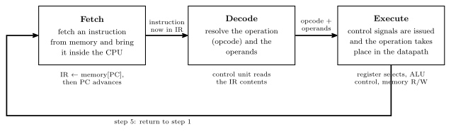
Figure 23: The cycle as a loop: a three-stage pipeline. Each box holds a one-line description of its stage, each arrow carries what the stage leaves behind for the next one, and the notes under the boxes summarise steps 1–4 above.
Step 2 advances the PC before the instruction executes, which is why a jump instruction works by overwriting the PC rather than by suppressing the increment.
The datapath
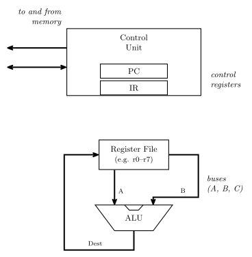
Figure 24: The datapath the cycle runs on. The control unit holds PC and IR and talks to memory; below it, the register file puts two values onto the A and B buses, the ALU combines them, and the result returns on the destination bus to be written back into a register.
The question this raises — and the one the control unit exists to answer — is how do we control this? Specifically:
- How do we tell the ALU what to do?
- How do we choose what register values are placed on the A and B buses?
- How do we choose which register receives the result from the destination bus?
- How do we know when to read or write memory?
Control signals
Each of those questions is answered by a bundle of wires out of the control unit. For a machine with 8 registers and the ALU of arithmetic-logic-unit:
| Signal | Width | Answers |
|---|---|---|
| A register select | 3 | which register drives the A bus (\(2^3 = 8\) registers) |
| B register select | 3 | which register drives the B bus |
| Destination select | 3 | which register the result is written back into |
| ALU control | 6 | what the ALU does — \(F_1\), \(F_0\), ENA, INVA, ENB, INC |
| Memory read/write | 1 | whether this is a read or a write |
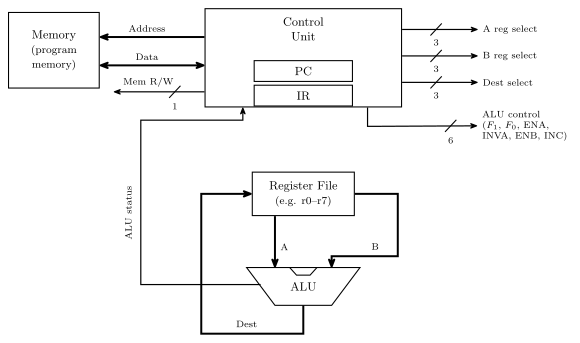
Figure 25: The same datapath with every control signal named. Added to the previous figure: the memory block, the Address, Data and Mem R/W labels, the five bundles with their widths, and the ALU status path back into the control unit. The bundles are drawn as labelled stubs: A/B/Dest select drive the register file, ALU control drives the ALU. Widths are marked with a slash and a number; the course also letters the width beside a plain arrow, and neither is fixed as the standard. Everything except the memory block sits inside the CPU.
Plus the address and data connections to memory itself. The widths are not arbitrary: three bits because there are eight registers, and six bits because the ALU has exactly six control inputs.
Control signals come from the control unit, which must generate them in the right order for a given instruction — and which instruction that is, is determined by the contents of the Instruction Register.
So a line of high-level code like r5 = r0 + r2 becomes: A select = 0, B select = 2, destination select = 5, ALU control = the \(A + B\) row of the combinations table, memory read/write idle.
Data influencing control
The IR is not enough. The control unit can’t operate without knowing something about the data — for example, if a for-loop variable is supposed to count from 10 down to 0, how does the control unit know when it gets there?
The answer is the status register: determined by ALU operations, it stores the status of the last ALU operation and is available to the control unit. This closes the loop — the ALU’s results feed back into the control unit and change what it does next, which is what makes conditional branching possible at all. It is the return path drawn in Figure 25, and it is what a source-level if (x < 0) compiles down to.
ALU status flags
The ALU emits, alongside its result, a summary of what happened during the last operation. Typically stored in a special purpose register called the STATUS register:
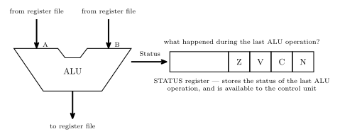
Figure 26: The ALU’s second output. The result goes back to the register file; alongside it the ALU reports what happened, and those flags land in the STATUS register where the control unit can read them. The ALU is drawn as a notched trapezoid here; the block diagram in the ALU note draws the same block as a plain rectangle, and the course uses both shapes. The register is drawn as four named cells at the right-hand end of a wider register. That is shorthand, not a bit-position claim — the AVR’s own SREG orders and numbers its bits differently, see the AVR architecture note.
| Flag | Name | Asks |
|---|---|---|
| Z | zero | was the last result 0? |
| V | overflow | did the last addition/subtraction overflow, assuming it was a two’s complement operation? |
| C | carry | was a carry out generated? |
| N | negative | was the result negative if considered as two’s complement — i.e. what is the sign bit? |
V and N both presuppose a two’s complement interpretation while C does not — the hardware computes all four regardless, and it is the program’s business to read the ones that mean something for the operation it just did. See binary-number-representations, and 2026-08-04-binary-arithmetic for the overflow rules V implements.
Worked example
What values are in the status register flags after the operation \(8_{10} - 9_{10}\) on a 5-bit ALU?
First, \(-9\) in 5-bit two’s complement: \(9 = 01001\), invert to \(10110\), add one to get \(10111\). Then add, tracking the carry into and out of the sign column:
\[\begin{array}{crl} \text{carry into MSB} \rightarrow & 0\phantom{0000} & \\ & 01000 & \\ + & 10111 & \\ \hline \text{carry out} = 0 \rightarrow & 11111 & \end{array}\]
The result is \(11111\), with no carry out of the top bit. So:
| Flag | Value | Why |
|---|---|---|
| Z | 0 | the result \(11111\) is not zero |
| C | 0 | no carry out of the most significant bit |
| V | 0 | the carry into the sign column and the carry out of it agree, both 0 — and indeed \(8 + (-9) = -1\) is comfortably in range for 5-bit two’s complement |
| N | 1 | the sign bit is 1 — the result is negative |
And indeed \(11111\) read as two’s complement is \(-1\), which is \(8 - 9\).
See also
- cpu-organisation · arithmetic-logic-unit
- binary-number-representations — two’s complement, overflow and the sign bit
- 2026-08-04-binary-arithmetic — the \(C_{in} \oplus C_{out}\) overflow test the V flag implements
- avr-architecture — the AVR’s own status register, bit by bit
- state-machines — the control unit is itself a state machine, sequencing signals for each instruction
- 2026-08-24-alu-and-control-unit — Lecture 9
Memory Models
The first of the four things that make up an ISA (instruction-set-architecture): how memory looks to the CPU. Four issues decide that — addressable cell size, alignment, address spaces and endianness — and every one of them is a decision the specification has to make, not something the hardware settles on its own.
Memory as addressable cells
Computer memory is conceptually a set of addressable cells:
- Each cell has a unique address (or cell number).
- Cells are usually 8 bits wide (i.e. hold one byte).
- Various cell widths have been used in the past — 8 bits is a convention, not a law.
Drawn as a table, the address indexes the rows and the cell width is how wide each row is:
| Address | ← cell width → |
|---|---|
| 0 | |
| 1 | |
| 2 | |
| 3 | |
| … |
A “4 × 3 memory” in that notation means 4 addresses of 3-bit cells — and \(4 = 2^2\), so two address bits. Built at gate level, it shows that “memory” at this level is nothing more exotic than flip-flops-and-latches and combinational-logic-blocks arranged into storage.
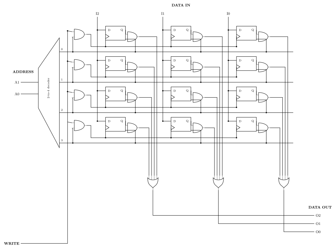
Figure 27: A 4 × 3 memory at gate level — four addresses of three-bit cells. Twelve D flip-flops in four rows of three: one row is one addressable cell. The decoder turns A1 A0 into exactly one row-select (word) line. Writing: the word line ANDed with WRITE clocks that row’s three flip-flops, so DATA IN (I2 I1 I0) — which is wired to every row’s D inputs all the time — is captured only by the selected row. Reading: each flip-flop’s Q is ANDed with its own word line and the three cells of a column are OR’d together, so the unselected rows contribute 0 and DATA OUT (O2 O1 O0) carries the selected row alone. The decoder is drawn as a trapezoid with the wide edge on the right, and the flip-flops as plain rectangles with a clock wedge on the lower-left edge, per this course’s conventions (csse2010-diagram-notation). The most significant bit, I2/O2, is the leftmost column.
A. Addressable cell size
Most common cell size is 8 bits (1 byte) — but not always.
The AVR is the counterexample sitting on the bench:
| AVR memory | Cell width |
|---|---|
| Data memory | 8 bits |
| Instruction (program) memory | 16 bits |
Which is why an AVR instruction is “one word” rather than “two bytes” — a program-memory address counts 16-bit cells.
The bus transports the content of a cell, but the data bus may be wider than one cell: it can retrieve several cells (addresses) at once. When it does, the address bus does not need to be as wide.
Bus sizes
For every doubling of the data bus width, remove the least significant bit of the address bus.
For a memory of \(2^n\) cells at 8 bits per cell — so an address size of \(n\) bits:
| Data bus | Address bus | Cells per transfer |
|---|---|---|
| 8 bits | \(n\) bits | one cell at a time |
| 16 bits | \(n-1\) bits | two cells at a time |
| 32 bits | \(n-2\) bits | four cells at a time |
The reason is that a wide transfer always moves an aligned group of cells. With a 16-bit data bus the memory only ever hands over cell pairs \((0,1), (2,3), (4,5), \dots\) — so the bottom address bit never selects anything, and naming the pair takes one bit fewer than naming the cell.
Worked example. A memory of 64 cells, 8 bits each, addressed 000000 … 111111:
\[64 = 2^6 \text{ cells} \implies 6\text{-bit addresses}\]
| Data bus | Address bus |
|---|---|
| 8 | 6 |
| 16 | 5 |
| 32 | 4 |
Read the two buses as a pair, not separately: widening one narrows the other by exactly as much.
Word addresses and byte addresses
The AVR’s 16-bit program-memory cells have one practical consequence. The program counter, jmp, call and every code label count words. But a table of constant bytes kept in flash is read a byte at a time by lpm, load program memory, and lpm takes a byte address in the Z register. Word \(w\) holds bytes \(2w\) and \(2w + 1\), with the low byte at the even address, which is the AVR being little endian (section D).
So turning a code label into a byte address means doubling it. Take the string Hello stored at word 2 by mesg: .db 72,101,108,108,111 (assembly-process):
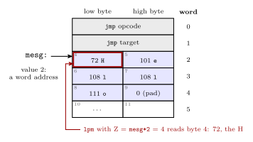
Figure 28: One region of program memory addressed two ways. Each row is a 16-bit word, numbered on the right, and each half is a byte, numbered inside its cell. The label mesg has the value 2 because labels in the code segment count words. Byte addressing counts the halves, low byte first, so word 2 starts at byte 4. That is why lpm is pointed at mesg*2: with Z = 4 it loads 72, the H. The five bytes of the string take two and a half words, and the last half word is a zero pad. Grey marks the jmp, blue the string and red the byte that lpm reads.
        ldi  ZH, high(mesg*2)   ; Z = 4: byte address of word 2
        ldi  ZL, low(mesg*2)
        lpm                     ; r0 <- 72, the H
Leaving out the *2 points Z at byte 2, the low byte of word 1, which is half of the jmp.
B. Alignment
Many architectures require natural alignment, e.g.
- 4-byte words starting at addresses 0, 4, 8, …
- 8-byte words starting at addresses 0, 8, 16, …
i.e. an \(n\)-byte value must start at an address that is a multiple of \(n\).
Taking an 8-byte word on a machine that fetches 8 bytes at a time:
| Where it sits | Reads needed | |
|---|---|---|
| Aligned | bytes 8–15, i.e. an 8-byte word at address 8 | 1 — it is exactly one fetched block |
| Non-aligned | bytes 12–19, i.e. an 8-byte word at address 12 | 2 — the top half of block 8–15, plus the bottom half of block 16–23 |
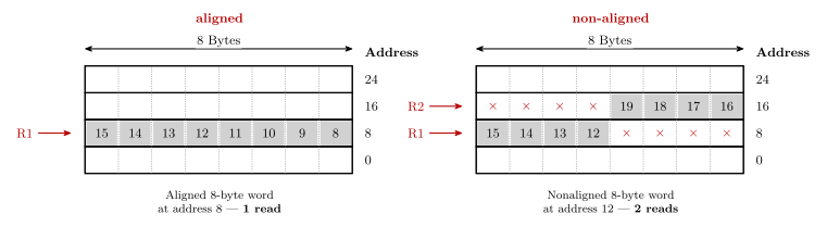
Figure 29: An aligned and a non-aligned 8-byte word. Four blocks of eight bytes; grey marks the bytes of the 8-byte word. On the left the word starts at address 8, so it is one block — one read. On the right it starts at address 12, so it takes the top half of the block at 8 and the bottom half of the block at 16 — two reads, marked R1 and R2. Two things about the drawing: addresses increase upward (unlike every other memory figure in the course, where they increase downward — see csse2010-diagram-notation on that inconsistency), and byte numbers within a row run high-to-low left to right. The × marks a byte in the fetched block that is not part of the word.
Alignment is often required because it is more efficient — the aligned case is always one read, the non-aligned case sometimes two, and the hardware that stitches two blocks together and extracts the middle is hardware that a machine demanding alignment simply does not need.
When alignment is not required — the Pentium IV
- Fetches 8 bytes at a time from memory (64-bit wide data bus).
- Alignment is NOT required, so the processor stays backwards compatible with earlier processors.
- A 4-byte word stored at address 4 takes 1 read (bytes 0 to 7).
- A 4-byte word stored at address 6 must read bytes 0 to 7 (one read) and bytes 8 to 15 (second read), then extract the 4 required bytes from the 16 bytes read.
Counting reads in general
A data bus \(w\) bytes wide delivers one aligned \(w\)-byte block per read. An \(n\)-byte value starting at address \(a\) therefore costs
\[\left\lceil \frac{(a \bmod w) + n}{w} \right\rceil \text{ reads}\]
The best case is \(n/w\) (rounded up), when the value starts on a block boundary; every other starting offset can push it one block further. So a value read from an arbitrary address costs either \(\lceil n/w \rceil\) or one more than that — which is why questions of this shape almost always answer “\(k\) or \(k+1\)” rather than a single number.
Worked example: an 8-byte value on a 16-bit data bus, no natural alignment required. Here \(w = 2\) and \(n = 8\):
| Starting address | Spans | Reads |
|---|---|---|
| Even | 4 aligned 2-byte blocks | 4 |
| Odd | 9 byte-positions, so 5 aligned blocks | 5 |
so the answer is 4 or 5. The odd case is the one to picture: one byte of the value sits alone at the top of the first block and one byte alone at the bottom of the last, and each of those still costs a whole read.
C. Address spaces
Many microprocessors have a single linear memory address space — the von Neumann architecture:
- e.g. \(2^{32}\) bytes numbered from 0 to \(2^{32} - 1\).
- (These may not be bytes — it depends on the addressable cell size.)
- Program and data share the one space.
However, the Harvard architecture has separate address spaces for instructions and data. The same numeric address means a different location depending on which space you are in, and an instruction says which one it means by what instruction it is.
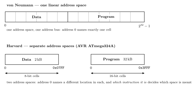
Figure 30: The two address-space models. Above: von Neumann — one linear space, so program and data are separated only by convention and address 0 names exactly one cell. Below: Harvard, in the AVR ATmega324A’s shape — two spaces, each starting at its own 0, with different sizes and different cell widths — and the cell width under each box is the whole reason the arithmetic below works out the way it does: 32 kB of program memory is \(2^{15}\) bytes but only \(2^{14}\) addresses, because each address there names a 16-bit cell. The end addresses follow from the sizes, so the data box ends at 0x07FF (\(2^{11}-1\), for 2048 bytes) rather than the 0x08FF of Figure 31, which is that 2 kB plus the 256 locations in front of it.
AVR ATmega324A is Harvard:
| Space | Size | Address width |
|---|---|---|
| Data | \(2^{11}\) (2048) bytes | 11 bits |
| Instruction | \(2^{14}\) 16-bit words — 16,384 instruction words = 32,768 bytes | 14 bits |
The arithmetic — convert to cells first, then take the logarithm:
\[\text{data: } 2\,\text{kB} = 2 \cdot 2^{10}\,\text{B} = 2^{11} \text{ cells (8-bit)} \implies 11 \text{ bits}\] \[\text{program: } 32\,\text{kB} = 2^{5} \cdot 2^{10}\,\text{B} = 2^{15}\,\text{B} = 2^{14} \text{ cells (16-bit)} \implies 14 \text{ bits}\]
The program-memory step is the one that catches people: 32 kB of flash is only \(2^{14}\) addresses, not \(2^{15}\), because each address names a 16-bit cell. Halve the byte count before taking the log whenever the cells are not bytes.
Laid out as a memory map (see avr-architecture for the rest of the chip):
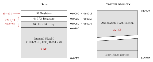
Figure 31: The ATmega324A’s two address spaces. Lowest address at the top, hex addresses outside on the right, grey fill on the coarsely-described regions, and the diagonal break across the flash meaning not to scale: that is this course’s memory-map convention (csse2010-diagram-notation). Marked in red: the register file is r0–r31, the 64 I/O plus 160 extended I/O registers are the 224 of avr-io-ports, the SRAM is 2 kB and the flash 32 kB.
Two details worth pinning down. 0x3FFF \(= 2^{14} - 1\), which is the 14 bits above. And the data space runs to 0x08FF — that is the 2 kB of SRAM plus the 256 locations (0x0000–0x00FF) that the register file and I/O registers occupy in front of it; the “\(2^{11}\) bytes” above is the SRAM itself, which is what the 11 bits size.
The assembler’s view: segments
An assembler treats each address space as a segment with its own location counter (assembly-process). On the ATmega324A there are three, because the EEPROM is a third address space alongside the two above:
| Segment | Directive | Address space | Cell | Counter starts at | The assembler can |
|---|---|---|---|---|---|
| code | .cseg |
program memory, flash, 32 kB | 16-bit word | 0x0000 |
place instructions and constants |
| data | .dseg |
data memory, SRAM | byte | 0x0100 |
only reserve space |
| EEPROM | .eseg |
EEPROM, 1 kB | byte | 0x0000 |
place constants |
Three consequences of separate spaces:
- The same number means different places. Address 0 is the reset
jmpin the code segment, registerr0in data memory and the first EEPROM byte in the EEPROM segment. - The units differ.
.org 0x0100in the code segment is word 256, which is bytes 512 and 513 of flash. In the data segment it is byte0x0100. - The data counter does not start at 0. The first 256 data addresses are the registers and I/O registers of Figure 31, so the first variable lands at
0x0100.
The data segment can only be reserved, not filled, because the assembler’s output is programmed into flash and EEPROM, which keep their contents, while SRAM starts empty at every power-up.
The memory behind each space
The three spaces are three different kinds of memory, and the kind explains how each is used (memory-technologies):
| Space | Technology | Volatile? | Erased and rewritten |
|---|---|---|---|
| Program memory | flash | no | electrically, a block at a time |
| Data memory | SRAM, flip-flops | yes | written a byte at a time, freely |
| EEPROM | EEPROM | no | electrically, one cell (byte) at a time |
The flash is divided into two blocks, the Application Flash Section and the Boot Flash Section of Figure 31. Because flash is erased a block at a time, a boot loader in the boot section can erase and rewrite the application section without erasing itself. Other AVR devices have one flash block, and some have more.
The register file and the SRAM sit at the top of the memory hierarchy. Unlike a desktop processor, the AVR has no cache: its SRAM is small enough and fast enough to keep up with the CPU directly.
D. Endianness
Different machines may support different byte orderings for a multi-byte value.
| Which end goes first (at the lowest address) | Used by | |
|---|---|---|
| Little endian | the little end — least significant byte | Intel microprocessors (Pentium etc.), and AVR |
| Big endian | the big end — most significant byte | SPARC, Freescale (formerly Motorola) microprocessors |
Most desktop/workstation/server CPUs produced since ~1992 are “bi-endian” (support both) — some switchable at boot time, others at run time, i.e. they can change dynamically.
Endianness only ever matters when a value spans more than one cell: reassembling it means knowing which cell was the low-order one.
Worked example
Given this memory:
| Address | Contents |
|---|---|
| 0 | 00001111 |
| 1 | 00110011 |
| 2 | 11011101 |
| 3 | 00101100 |
| Read | Value | Why |
|---|---|---|
| the 1-byte word at address 1 | 00110011 |
one cell — endianness does not apply |
| the 2-byte word at address 0, big endian | 00001111 00110011 |
big end first, so address 0 holds the most significant byte |
| the 2-byte word at address 2, little endian | 00101100 11011101 |
little end first, so address 2 holds the least significant byte and address 3 the most |
The mechanical way to do these without getting turned around: write the addresses the value occupies in increasing order, then assemble the answer most-significant-byte first. Big endian reads the addresses forwards; little endian reads them backwards.
See also
- instruction-set-architecture — the four pillars this is the first of
- avr-architecture — the ATmega324A’s two address spaces in full
- addressing-modes — how an instruction names a memory location
- binary-number-representations · flip-flops-and-latches · combinational-logic-blocks
- assembly-process — segments, location counters, and
.dbpacking two bytes to a word - compilation-and-linking — where a C compiler puts globals, locals and the heap in data memory
- memory-technologies — flash, SRAM and EEPROM as technologies, and why sizes are powers of 2
- memory-hierarchy-and-cache — registers, cache, main memory and disk, by speed and cost
- 2026-08-31-instruction-set-architecture-part-1 — Lecture 11 · 2026-10-08-assembly-process — Lecture 20 · 2026-10-22-memory-disks-and-files — Lecture 24
Procedures and the Stack
What a procedure is at the machine level, how call and ret get into it and back out, and the stack — the structure that makes returning possible from any depth of nesting, holds saved registers and arguments, and has to be set up before any of that works. First met in 2026-09-14-flow-of-control; branches and jumps are in avr-branches-and-jumps, and data memory, where the stack lives, is in memory-models and avr-architecture.
Procedures
A procedure is a group of instructions that performs some task, which
- may have operands — arguments or parameters,
- may produce result(s),
- can be invoked (called) from multiple places in a program — even from within itself, a recursive procedure — and
- after invocation, control returns to the statement after the call.
It is the same thing as a C function (c-language-basics), a Python function, a Java method, or a subroutine; the names differ by language, the mechanism does not. Good use of procedures is most of what makes a program of any size readable, and the AVR C compiler turns every function into exactly what follows.
The return is the part with machinery behind it. A jump goes somewhere; a call goes somewhere and remembers where it came from, so that a ret at the far end can come back — to a different place each time, depending on who called.
call and ret
| Instruction | Size | Cycles | |
|---|---|---|---|
call label |
direct call — target is an absolute address | 32-bit | 4 |
rcall label |
relative call — target is PC ± 2 K words | 16-bit | 3 |
icall |
indirect call — target is the address in Z | 16-bit | 3 |
ret |
return to the instruction after the most recent call | 16-bit | 4 |
The three calls mirror jmp, rjmp and ijmp exactly — same reach, same sizes — and each costs one cycle more than its jump. That cycle is the push. What a call does, in order:
- compute the return address — the address of the instruction after the call;
- push it onto the stack;
- load the PC with the target.
And ret undoes it: pop the top of the stack into the PC. Nothing in the procedure needs to know who called it, because the address to go back to was left on the stack by the caller.
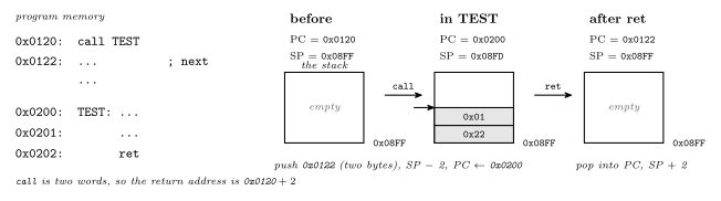
Figure 32: A call and its return, followed through the three registers involved. The PC, the stack pointer and the top of the stack are shown before the call, during the procedure and after the return, with example addresses. call records the address of its own successor on the stack and lowers the stack pointer by two, because a program-memory address needs two bytes; then it loads the PC with the procedure’s address. ret reverses both steps and execution resumes at the recorded address, which is the instruction after the call. The procedure body never touches the return address, so it does not matter what the procedure does in between, provided it leaves the stack as it found it.
Why a stack
The return address has to be stored somewhere. There are three candidates:
| Where | Fails when |
|---|---|
| A single fixed register or memory address for all calls | a procedure calls another procedure — the second call overwrites the first’s return address, and the outer procedure can never return |
| One memory location per procedure | a procedure calls itself — recursion needs two live return addresses for one procedure |
| A stack | never, until memory runs out |
A stack is a last-in, first-out store: push puts a value on top, pop takes the top value off. Calls and returns nest — the most recent call is always the first to return — so a stack of return addresses always has the right one on top. Nested calls are drawn step by step in 2026-09-14-flow-of-control.
The AVR stack
On the AVR the stack is simply a region of data memory (memory-models), and the stack pointer is a 16-bit address held in two I/O registers, SPH:SPL, that says where the top currently is. Two conventions fix how it works:
- The stack grows downward. A push stores at the address in
SPand then decrementsSP; a pop incrementsSPand then loads from it. SoSPalways points at the next free cell, just below the most recently pushed byte. - It starts at the top of SRAM. Program variables are allocated from the bottom of SRAM upward; the stack is started at the last address,
RAMEND(0x08FFon the ATmega324A), and grows down toward them. Neither has to know in advance how much room the other needs.
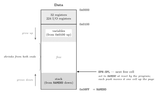
Figure 33: Where the stack lives in the ATmega324A’s data memory. The general-purpose registers and I/O registers occupy the first 256 addresses; SRAM begins at 0x0100. Global variables are laid out from the bottom of SRAM upward, and the stack starts at the top, RAMEND, and grows downward toward them, with SPH:SPL holding the address of the next free cell. The gap between them is the free memory, and it shrinks from both ends: every nested call, every push and every local variable of a running function takes cells off the top, and the stack overflows when it reaches the variables — silently, since nothing checks. That is why the stack pointer must be set to RAMEND before the first call: the reset value would put it somewhere else entirely.
Initialising the stack pointer
An assembly program must initialise the stack before using it. These four lines belong at the top of RESET: in any program that calls anything:
.def temp=r16
    ldi  temp, low(RAMEND)
    out  SPL, temp
    ldi  temp, high(RAMEND)
    out  SPH, temp
RAMEND is defined by the device include file (avr-io-ports), and low()/high() split the 16-bit value because SPL and SPH are two separate 8-bit I/O registers. In C the compiler emits this itself as part of the start-up code that runs before main; it is one of the things a C program on the AVR gets for free and an assembly program does not. The RESET template in avr-program-structure does not include it only because nothing in the Lab 10 programs made a call.
push and pop
The two stack instructions are also available directly:
| Cycles | ||
|---|---|---|
push rr |
store rr at SP, then SP ← SP − 1 |
2 |
pop rd |
SP ← SP + 1, then load rd from SP |
2 |
Their main use is saving registers a procedure is about to clobber, so that the caller gets them back unchanged:
TEST:
    push r16           ; save what the caller had in r16 and r17
    push r17
    ...                ; use r16, r17 freely
    pop  r17           ; restore — in REVERSE order
    pop  r16
    ret
The order matters because the stack is LIFO: the last register pushed is the first one back. And the count matters even more — every push must be matched by a pop before the ret, because ret pops whatever is on top and treats it as the return address. One push too many and the procedure returns to an address made of a register’s contents; one too few and it returns into the middle of the saved data.

Figure 34: Saving and restoring registers around a procedure body, with the stack drawn after each instruction. The return address is already on the stack when the procedure starts; the two pushes go on top of it, and the two pops must come off in the reverse order to land in the right registers. When ret runs the return address is back on top, exactly as call left it. If the pops were in the same order as the pushes, r16 and r17 would come back swapped; if one pop were missing, ret would pop the saved r16 and jump to whatever address that byte pair happened to spell.
Arguments and results
Arguments are passed and results returned in one of two ways: in registers, or on the stack.
- Registers are the fast way for a few small values: the caller puts the argument in an agreed register before the
call, the procedure reads it there and leaves its result in an agreed register for the caller to pick up. Agreement is the whole trick — both sides must use the same register, and a procedure that uses registers for arguments cannot also expect them preserved. - The stack is the general way: the caller pushes the arguments, then calls; the procedure finds them on the stack just above the return address, and results can be returned the same way or in registers. The return address, the arguments and any saved registers and locals together are the procedure’s stack frame. It costs pushes and pops, but it works for any number of arguments and for recursion, since every live call has its own frame.
The AVR C compiler uses both: the first few arguments of a function travel in registers, r24 down, and the rest on the stack, and a function’s local variables live in its stack frame. Those details are the compiler’s convention, and they are why a C function call is not free — see the main costs in c-language-basics.
A C function’s stack frame
A C compiler puts a function’s local variables in its stack frame, next to the return address and any arguments passed on the stack. The frame is pushed when the function is called and popped when it returns. A local therefore exists only while its call is running, and each call, including each level of a recursion, gets its own copy at its own address. An optimising compiler keeps a small local in a register when it can. The frame is where it goes when it needs memory, and the lifetime is the same either way.
In address order, from high to low, which is the order they are pushed:
- arguments, pushed by the caller before the call, if any are passed on the stack;
- the return address, pushed by
call; - locals, made by the function itself when it starts.
A static local is not in the frame. It is stored with the globals, at a fixed address, so it outlives the call and still holds its value the next time the function runs. Globals sit at the bottom of SRAM, the heap grows up above them, and the stack grows down from RAMEND. A stack that grows far enough to meet the heap has overflowed. How the compiler lays out the whole data memory is in compilation-and-linking.
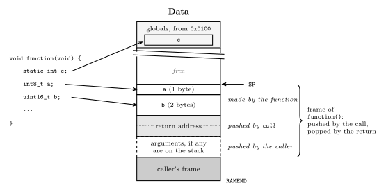
Figure 35: The stack frame of a C function while it runs, with the lowest address at the top as in the course’s memory maps. The caller pushed any stack arguments, call pushed the return address, and the function made room for its locals a and b above that. SP points at the next free cell, just above the frame. When the function returns, the whole frame is popped and SP goes back to where it was before the call, so a and b no longer exist. The static local c is not in the frame at all. It is stored among the globals at a fixed address, which is why it keeps its value from one call to the next.
The stack and interrupts
An interrupt uses the same stack in the same way. The hardware pushes the return address exactly as call would, and the handler’s reti pops it, like ret (avr-interrupts, 2026-09-21-interrupts). Three things follow:
- The stack pointer must be set before interrupts are enabled, not merely before the first
call. An assembly program with no procedures at all still needsSPinitialised once it uses an interrupt. - A handler’s pushes and pops must balance, and it must restore every register it uses. This is the same rule as for a procedure, but stricter: an interrupt can arrive between any two instructions, so there is no caller to agree anything with (polling-and-interrupts).
- Every interrupt that is being handled holds stack space: two bytes of return address plus whatever its handler pushes, and more again if handlers are allowed to nest.
Pitfalls
- Forgetting to initialise
SPin an assembly program. The firstcallpushes to wherever the reset value points; theretthen reads garbage. In C, not a concern. - Unbalanced push/pop inside a procedure — see Figure 34.
retdoes not check what it pops. - Stack overflow. Deep recursion, or big local arrays in C, walk the stack down into the heap and the variables. Nothing on the chip detects it; the symptom is variables changing value for no visible reason.
- Returning a pointer to a local. The local’s frame is popped by the return, so the pointer points at stack space that the next call will reuse.
- Clobbering the caller’s registers. A procedure that uses
r16without saving it changesr16for whoever called it. Either save and restore, or document which registers the procedure destroys — and be consistent.
See also
- avr-branches-and-jumps —
jmp,rjmp,ijmp, and the conditional branches - avr-program-structure — the
RESETtemplate the stack initialisation goes into - memory-models · avr-architecture — data memory,
RAMEND, and the I/O registersSPH/SPL - avr-instructions —
push,pop,call,retamong the rest - c-language-basics — functions in C, which compile to exactly this
- compilation-and-linking — where the compiler puts globals, locals, statics and the heap · 2026-10-15-compilation-and-linking — Lecture 22
- avr-interrupts · polling-and-interrupts — the same stack, used by the hardware
- 2026-09-14-flow-of-control — Lecture 15 · 2026-09-21-interrupts — Lecture 17, the stack under interrupts