Lecture 22 — Compilation and Linking
What happens between a C program and the machine code that runs it. The note covers compiled against interpreted languages, with Java and Python’s bytecode in between; where a C compiler puts global, local and static variables; why programs are built from separately compiled object files, and the six sections of one; how the linker relocates and resolves addresses; libraries, and how a header differs from a library; and dynamic linking. It picks up from the assembler’s two passes in 2026-10-08-assembly-process. The reference note is compilation-and-linking. Where variables live is also in procedures-and-the-stack and c-language-basics, and headers against libraries in c-preprocessor-and-avr-headers.
Goals
- Tell compiling from interpreting, and place Java and Python’s bytecode and just-in-time compilation between the two.
- Say where a C compiler puts global, local and
staticvariables in the AVR’s data memory. - Explain why programs are compiled into separate object files, and what each of the six sections of an object file holds.
- Link modules by hand: lay them out in link order, relocate their internal addresses and resolve their external ones.
- Tell a header file from a library, and static linking from dynamic linking.
Compilation
A program has to be converted to machine code before it can run. The processor only fetches, decodes and executes machine instructions (fetch-decode-execute-cycle). The conversion is called compilation, and it often goes by way of assembly language: the compiler writes assembly, and the assembler turns that into machine code.
Not every program is compiled, though.
Interpretation
Some languages are interpreted, Python, Java and MATLAB among them. The high-level program is never turned into machine code. It is the input to an interpreter, a program that reads the source and carries out each statement as it reaches it. What runs on the processor is the interpreter, which is machine code like any other program. Many interpreters first turn the source into bytecode, a compact instruction format of their own, and then interpret that.
The trade-off:
- + Portability. The program is not tied to any instruction set. It runs on any machine that has an interpreter for its language.
- − Slow. Each time a statement runs, the interpreter works out again what it means, which costs many of its own instructions. In a loop it does that on every pass. A compiled program did that work once, before it started.
Java and Python
Java, and Python in the same way, takes a route between the two.
- The source is “compiled”, but into bytecode, not machine code. Bytecode is the instruction set of an imaginary machine, so it is portable across all platforms: the same file runs anywhere.
- The bytecode is the input to the Java Virtual Machine, an interpreter for bytecode, which runs on the processor.
- To recover the speed, the virtual machine just-in-time compiles the parts that run most often into real machine code while the program is running. From then on those parts run on the processor directly.
Numba does the third step for Python: it compiles a chosen Python function to machine code the first time it is called. More in compilation-and-linking.
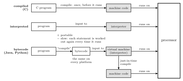
Figure 1: Three ways from a program to the processor. The grey boxes are machine code, which is the only thing a processor can run. A compiled program becomes machine code before it runs. An interpreted program never does: the interpreter is what runs, and it carries out the program’s statements one at a time, which is portable but slow. Java and Python compile to bytecode, which is the same on every platform, and a virtual machine interprets it. The virtual machine also compiles the busiest parts to machine code while the program runs, and from then on those parts run on the processor directly.
What compiling C involves
In a simplified view, compiling a C program is three jobs.
- Mapping variables to memory: giving every variable a place.
- Translating C code into assembler instructions: each statement becomes however many instructions it needs.
- Turning assembler instructions into machine code, which is the assembly process (assembly-process).
So the route is C → assembly → machine code. Some compilers go straight from C to machine code and skip the assembly text, but the jobs are the same. Job 1 is the subject of the next two sections. The whole chain from source file to flash is drawn in compilation-and-linking.
Global variables
Variables come in two kinds as far as memory is concerned. Global variables are declared outside every function. Local variables are declared inside one.
A global can be used by any function at any time, for the whole run, so the compiler gives it a fixed address in data memory. It works out the addresses itself, in the same way an assembly programmer reserves space with .dseg and .byte. On the ATmega324A the data space begins with 32 registers (addresses 0 to 31), 64 I/O registers (32 to 95) and 160 extended I/O registers (96 to 255), so the first byte free for variables is 256, 0x0100 (memory-models).
Worked: placing three globals
Where do these three globals go in the ATmega324A’s data memory, and what assembly reserves the same space?
/* global variables */
int count;
char c;
static int a;
Sizes first. On the AVR an int is 16 bits, 2 bytes, and a char is 8 bits, 1 byte (c-language-basics).
Then the addresses, one after another from 256 in the order declared. That is one layout a compiler may choose, since the order is up to the compiler.
| Variable | Size | Addresses |
|---|---|---|
count |
2 bytes | 256 and 257 |
c |
1 byte | 258 |
a |
2 bytes | 259 and 260 |
The next free byte is 261.
The assembly that reserves the same bytes:
.dseg               ; data segment: starts at the first SRAM byte, 256
count:  .byte 2     ; 256-257
c:      .byte 1     ; 258
a:      .byte 2     ; 259-260
.org 500
b:      .byte 1     ; 500
.byte n reserves \(n\) bytes and gives the first one the label’s name. .org moves the location counter, so a variable can be put at a chosen address. Here b is at 500, and 261 to 499 are left unused. That is something the assembly programmer decides. The C programmer leaves every address to the compiler.
And static? On a global, static does not change where the variable is stored: a is placed exactly like count. It makes the name private to this source file, so no other file can link to a (compilation-and-linking).
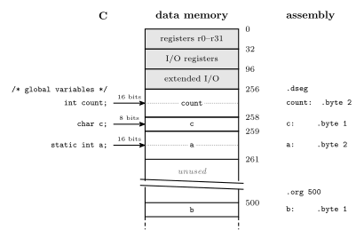
Figure 2: Three global variables placed in the ATmega324A’s data memory, with the lowest address at the top and decimal addresses on the right. The registers and the two banks of I/O registers fill addresses 0 to 255, so the globals start at 256 (0x0100). Each takes as many bytes as its type: two for an int and one for a char. On the right is the assembly that reserves the same bytes. In assembly, .org can put a variable at any address, here 500, leaving the bytes in between unused. The break in the column means the gap is not drawn to scale.
Local and static variables
A local variable exists only while its function is running. Each call gets a fresh copy, which is what makes recursion work, so a local cannot have a fixed address. It lives in the call’s stack frame instead, which holds the call’s arguments, its local variables and its return address.
When main executes call TEST, the frame for TEST is pushed onto the stack. When TEST reaches ret, the frame is popped and its locals are gone. The stack is described in procedures-and-the-stack.
The whole data memory then looks like this, from the lowest address up:
- registers r0 to r31, the I/O registers and the extended I/O registers, up to address 255;
- the globals, from 256;
- the heap, from which
malloc()hands out memory while the program runs, growing toward higher addresses; - free memory;
- the stack, which starts at the top of SRAM and grows down toward the heap. The stack pointer
SPmarks its current end, and the frames of all running calls sit betweenSPand the top.
If the stack grows down far enough to meet the heap, that is a stack overflow, and nothing stops it. This layout is drawn in compilation-and-linking.
Worked: where three variables of one function live
In this function, where is each of
a,bandcstored, and for how long?void function(void) { int8_t a; uint16_t b; static int c; ... }
ais a local, 1 byte. It is infunction’s stack frame. It is created whenfunctionis called and is gone at the return.bis a local, 2 bytes. It is also in the frame, so the frame holds 3 bytes of locals next to the 2-byte return address.cis declared inside the function but markedstatic. It is not in the frame. It lives among the globals, at a fixed address from 256 up, for the whole run. Onlyfunctioncan use the namec, but its value survives from one call to the next.
So if function is called twice, a and b start out with whatever happens to be on the stack each time, while c still holds what the first call left in it. The frame itself is drawn in procedures-and-the-stack.
Compiling C into object files
Compiling a C program runs into the same problem as the assembly process: there are names whose addresses are not yet known.
- The compiler often produces object files (
.o) as an intermediate step. Assemblers can produce object files too. - All the object files are generated first. Each of the program’s own
.cfiles is compiled, with its.hfiles and macros already expanded by the preprocessor, and the libraries arrive as object files that were compiled long ago. - Then they are all linked together, and the final details, such as memory locations, are worked out at that point.
An object file is machine code plus information. Suppose there are three source files, and the third defines a procedure TEST at its address 80. Each file is compiled as if it started at address 0, so in its object file TEST is only “80 from the start of this module”. The first file calls TEST but cannot know where TEST will end up, because that depends on where the linker puts the third module. So the object file records that the call needs TEST’s address. Once the linker has laid the modules out end to end, the third module’s start is known, TEST is that start plus 80, and the call is filled in.
Why object files
It is often useful to compile or assemble modules separately and then link them together. Change one file and only that file has to be compiled again.
The consequence is that, at compile time, nobody knows where the code will end up, meaning the addresses it will occupy. Once the location is known, the code has to be fixed. Code that carries the information needed for that is a relocatable object module. “Object module” and “object file” are used interchangeably.
The six sections of an object file
An object file is made of six sections, numbered from the bottom up. The structure is drawn in compilation-and-linking.
| Section | Holds | |
|---|---|---|
| 6 | End of module | (perhaps) a checksum to catch errors; the address at which to start execution |
| 5 | Relocation dictionary | the addresses in section 4 that need relocating |
| 4 | Machine instructions and constants | the code segment; the data segment, both initialised and uninitialised data |
| 3 | External reference table | symbols used here but defined elsewhere, and the instructions that use them |
| 2 | Entry point table | symbols defined here that other modules may use, with their addresses |
| 1 | Identification | the module’s name; where the other sections are in the file; the assembly date |
There are many different object file formats, among them a.out, COFF and ELF. ELF is what the AVR GCC toolchain produces. DWARF, often listed with them, is a format for debugging information, usually stored inside ELF files.
1. Identification section. The name of the module, the location of the other sections in the file, and the assembly date. The linker needs the locations to find everything else.
2. Entry point table. The list of symbols defined in the module that other modules may reference, with their values. The values are addresses: procedure entry points and variables. The addresses are relative to the beginning of this object module. For example, a file that defines a procedure called abs_value at address 10 lists abs_value with the value 10.
3. External reference table. The list of all symbols that are used in the module but not defined in it: procedure names and variables defined in some other module. Against each one is the list of instructions which use that symbol, the places that will need its address filled in.
4. Machine instructions and constants. The assembled code and constants, as a code segment and a data segment with both its initialised and uninitialised data. The addresses referenced in this code are not correct, because they assume the module starts at 0. They need relocation.
5. Relocation dictionary. The list of addresses of code and data in section 4 that need to be relocated. When the module is placed, a relocation constant is added to the instruction or data at each of these addresses, with different constants for code and data.
6. End of module. Possibly a checksum, to catch errors, and the address at which to start execution.
Worked: the tables for two modules
Module A defines a procedure
SUMat its address 80, and calls and jumps to a procedureX. Module B definesXat its address 71, and callsSUM. Write each module’s entry point table and external reference table.
Defined here and offered to others goes in the entry point table, with the address relative to the module’s own start. Used here but defined elsewhere goes in the external reference table, with the instructions that use it. In this example A’s call X is at 12, its jmp X at 40, and B’s call SUM at 30.
| Module | Entry point table | External reference table |
|---|---|---|
| A | SUM at 80 |
X: used by the call at 12 and the jmp at 40 |
| B | X at 71 |
SUM: used by the call at 30 |
Each symbol is defined in one module and used in the other. SUM is an entry point of A and an external reference of B, and X is an entry point of B and an external reference of A. Neither module can finish its instructions alone. The linker finishes them by matching every external reference against an entry point.
Worked: where does X end up?
Module A’s code is 100 words and its data 30 bytes. A and B are linked in the order A, then B, with code and data each starting at 0.
Xis at 71 in B. What are B’s relocation constants, what isX’s final address, and what do the instructions that useSUMandXbecome?
B’s relocation constants. B’s code goes straight after A’s code, and B’s data straight after A’s data:
- code constant = A’s code size = 100
- data constant = A’s data size = 30
The two constants differ because A’s code and A’s data are different sizes. That is why the relocation dictionary has to say, for each address, whether it is a code address or a data address.
X’s final address is its offset in B plus B’s code constant: \(100 + 71 = \mathbf{171}\).
The instructions.
- A’s
call Xat 12 andjmp Xat 40 are resolved: the linker looksXup and writes 171 into both. - B’s
call SUMmoves to \(100 + 30 = 130\) and is resolved too. A is first, so its constant is 0, andSUMstays at 80. - If B contained a branch to its own address 71, that branch would be in B’s relocation dictionary and would be relocated: \(71 + 100 = 171\). It lands in the same place, by adding a constant this time, because the target is inside the module being moved.
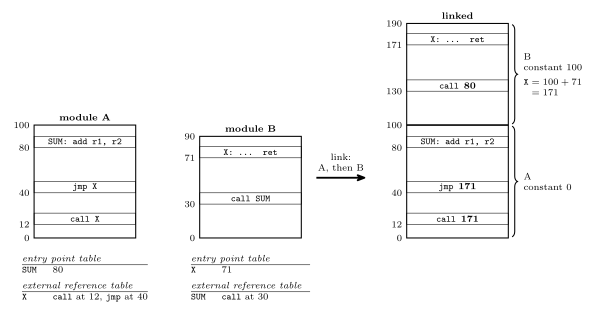
Figure 3: Two modules that each use a procedure the other defines, before and after linking, with addresses increasing up the page. Each module is assembled from 0. Its entry point table lists what it offers, with addresses relative to its own start, and its external reference table lists what it needs and which instructions need it. Linking A first and then B gives B a code relocation constant of 100, A’s size. X moves from 71 to 171, and the call and jump in A are filled in with 171. A’s constant is 0, so SUM stays at 80, and that is the address the call in B receives. The bold operands are the ones the linker wrote.
The linker and libraries
The linker combines object modules into an executable binary program, which is machine code. Each source procedure, in C or in assembly, goes through a translator (a compiler or an assembler) and becomes an object module. The linker takes all the object modules, plus whatever it needs from a library, and produces the one executable. The chain is drawn in compilation-and-linking.
A library is
- a collection of object files with an additional index, which tells the linker which member defines which symbol, and
- a collection of useful functions and procedures, ready to link.
The principle is not to reinvent the wheel, and to use library code where possible. The standard C library is the usual example. It provides:
- standard input and output,
- string handling,
- date and time functions,
- general utilities.
More in compilation-and-linking.
Header files against the library
A header file (.h) is not the library. A header file
- defines useful preprocessor macros,
- declares the functions that are in the library, as function prototypes, and
- declares the variables that are available externally, with
extern.
The library is the collection of object files that implements the functions.
A prototype tells the compiler the name, the argument types and the return type, which is enough to check a call and generate it. It contains no code. The code is in the library, and it is the linker that joins it on. The header goes to the compiler, by way of the preprocessor, and the library goes to the linker. Forgetting the header shows up when compiling, as an “implicit declaration” of the function: a warning from older compilers, an error from newer ones. Forgetting the library shows up when linking, as an “undefined reference”. See c-preprocessor-and-avr-headers.
Linking: relocating and resolving
Linking is a similar problem to assembling. It has the external reference problem: symbols are used before their values are known. A module can call a procedure in a module the linker has not read yet. So the linker needs two passes as well, in the same way the assembler does (assembly-process). The first pass places every module and collects every entry point. The second pass patches the code.
When modules are joined together, addresses need relocating or resolving.
- Relocating means adding some constant value: the module’s starting address, added to an address that points within the module.
- Resolving means finding the value of an “external” address: one that points into a different module, looked up from the entry points the linker collected.
The passes are described step by step in compilation-and-linking.
Worked: linking modules A and B
Four object modules are each assembled from 0. Module A (length 400) holds
BRANCH TO 200at 0,MOVE P TO Xat 200 andCALL Bat 300. Module B (length 600) holdsBRANCH TO 300at 0,MOVE Q TO Xat 300 andCALL Cat 500. Module C (length 500) begins withBRANCH TO 200. The modules are linked in the order A, B, C, D, after 100 words of start-up code. Where does B start, and what does each instruction of A and B become?
Where everything goes. The start-up code fills 0 to 99, so A starts at 100. A is 400 long, so it fills 100 to 499 and B starts at 100 + 400 = 500. B is 600 long, so C starts at 500 + 600 = 1100. The relocation constants are +100 for A and +500 for B.
Each instruction. An instruction at offset \(o\) in a module starting at \(s\) is now at \(s + o\).
| Now at | Was | Becomes | How |
|---|---|---|---|
| 100 | A: BRANCH TO 200 |
BRANCH TO 300 |
relocate, +100 |
| 300 | A: MOVE P TO X |
unchanged | no code address |
| 400 | A: CALL B |
CALL 500 |
resolve: B starts at 500 |
| 500 | B: BRANCH TO 300 |
BRANCH TO 800 |
relocate, +500 (100 + 400) |
| 800 | B: MOVE Q TO X |
unchanged | no code address |
| 1000 | B: CALL C |
CALL 1100 |
resolve: C starts at 1100 |
| 1100 | C: BRANCH TO 200 |
BRANCH TO 1300 |
relocate, +1100 |
Check that nothing broke. A’s branch at 100 now targets 300, which is exactly where A’s MOVE P TO X went. B’s branch at 500 targets 800, where B’s MOVE Q TO X went. A relocated branch still lands on the same instruction, because the branch and its target moved by the same amount. A call to another module is not fixed by adding A’s constant, though. CALL B needs B’s start, which only the layout of the whole program determines.
Finishing the job with D (length 300, at 1600) gives CALL D → CALL 1600 and D’s BRANCH TO 200 → BRANCH TO 1800. The complete table, and a drawing of the program after each of the linker’s two passes, are in compilation-and-linking.
Worked: where does module 2 start?
Modules are linked in order 3, 2, 1 starting at program address 62 and data address 256. At what program (code) address will module 2 start?
Module c-seg size (words) d-seg size (bytes) 1 45 17 2 67 5 3 100 25 A. 62 B. 87 C. 107 D. 146 E. 162 F. 229
Answer: E, 162.
The question asks about the code address, so only the c-seg column matters. In the order 3, 2, 1, module 3 goes first, from 62. It takes 100 words, 62 to 161, so module 2 starts at
\[62 + 100 = 162.\]
The full layout, with both memories:
| Module | Code (words) | Data (bytes) | Code constant | Data constant |
|---|---|---|---|---|
| 3 | 62 to 161 | 256 to 280 | +62 | +256 |
| 2 | 162 to 228 | 281 to 285 | +162 | +281 |
| 1 | 229 to 273 | 286 to 302 | +229 | +286 |
The next free code word is 274 and the next free data byte is 303.
Where the wrong answers come from:
- A, 62, is where module 3 starts. It is the first module in the order, not module 2.
- B, 87, is \(62 + 25\): module 3’s data size added to the code start.
- C, 107, is \(62 + 45\): module 2’s start if the modules were linked in the order 1, 2, 3.
- D, 146, matches no boundary in either memory.
- F, 229, is where module 1 starts, after module 2 rather than before it.
Why 62 and 256? On the ATmega324A, program words 0 to 61 hold the interrupt vector table, so 62 (0x003E) is the first word free for code (avr-interrupts). Data addresses 0 to 255 are registers and I/O, so 256 (0x0100) is the first byte of SRAM. Code is counted in words because each program memory location holds a 16-bit word. Data is counted in bytes because each data memory location holds one byte (memory-models).
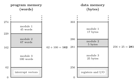
Figure 4: Three modules linked in the order 3, 2, 1, with addresses increasing up the page. Code and data are laid out separately, each in its own memory and its own units: words of program memory from 62, the first word after the interrupt vector table, and bytes of data memory from 256, the first byte of SRAM. Every module starts where the module before it in link order ends, so module 2’s code begins after module 3’s 100 words, at 162, and its data after module 3’s 25 bytes, at 281. Those two starts are module 2’s relocation constants. The heights are not to scale.
Dynamic linking
So far, all the object code, library and main program alike, is linked into one binary before the program runs. That is static linking.
Alternatively, linking can happen at run time: a library procedure is linked when it is first called. The executable contains only a reference to it, and the library stays in a file of its own. DLLs on Windows work this way.
The advantages:
- It saves space. The libraries are not linked into the binary executable, and every program that uses a library shares the one copy.
- The library can be updated independently of the programs that use it, and a fix reaches all of them without relinking.
The second is also a disadvantage. A program can break because something else installed a different version of a DLL it depends on. On earlier versions of Windows this happened often enough to be called “DLL hell”.
An AVR program has no operating system to do the run-time linking, so everything is linked statically. The two are compared side by side in compilation-and-linking.
See also
- compilation-and-linking — the reference note: the toolchain, variables in memory, the object file, both passes of the linker, libraries, dynamic linking
- assembly-process · 2026-10-08-assembly-process — the assembler’s two passes, the problem the linker repeats one level up
- procedures-and-the-stack — stack frames,
call,ret, push and pop - c-language-basics — how big each type is, and where globals, locals and statics live
- c-preprocessor-and-avr-headers —
#include, macros, and the header against the library - memory-models · avr-interrupts — the data map from 256 and the vector table that ends at 61
- 2026-10-19-floating-point-numbers — Lecture 23