Compilation and Linking
How a C program turns into the machine code in the AVR’s flash. This note covers compiling against interpreting, where the compiler puts global, local and static variables, object files and their six sections, the linker’s two jobs (relocating and resolving), libraries, how header files differ from libraries, and static against dynamic linking. The assembler’s part, with its two passes and symbol table, is in assembly-process. First met in 2026-10-15-compilation-and-linking.
Compiled or interpreted
A processor runs machine code and nothing else. The fetch-decode-execute cycle (fetch-decode-execute-cycle) reads instruction words from memory, and nothing in it knows the program was once written in C. A program in a high-level language reaches the processor in one of two ways.
- Compilation translates the whole program into machine code before it runs, often by way of assembly language. The machine code then runs directly on the processor. C works this way.
- Interpretation never turns the program into machine code. Another program, the interpreter, reads the source and carries out each statement when it gets to it. The interpreter is itself machine code, and it is the interpreter that the processor runs. Python, Java and MATLAB work this way.
| Compiled | Interpreted | |
|---|---|---|
| What the processor runs | the program’s own machine code | the interpreter’s machine code |
| When translation happens | once, before the program runs | every time a statement is executed |
| Speed | fast | slow |
| Portability | the machine code suits one processor only | runs anywhere an interpreter exists |
Why interpreting is slow. Every time a statement is executed, the interpreter has to work out again what the statement means and then carry it out. That costs many of its own instructions per statement, and inside a loop it is repeated on every pass. A compiler does that work once, ahead of time.
Why it is portable. The program never becomes machine code, so nothing in it is tied to one instruction set. Moving it to a new processor only needs an interpreter built for that processor.
Bytecode and just-in-time compilation
Java and Python take a route in between. The source is first compiled, but not into machine code. It becomes bytecode, the instruction set of an imaginary machine. Bytecode is the same on every platform, so a compiled Java program is portable across all of them.
The bytecode is then run by a virtual machine, which is an interpreter for bytecode. The Java Virtual Machine is the one for Java. Running bytecode is faster than interpreting source text, because the parsing has already been done, but it is still interpretation.
To win back the speed, the virtual machine watches which parts of the program run most often and compiles them into real machine code while the program is running. This is just-in-time (JIT) compilation. Once a part has been JIT-compiled, it runs directly on the processor like compiled code. Standard Python interprets its bytecode, and a JIT compiler such as Numba can compile chosen Python functions to machine code in the same way.
The toolchain
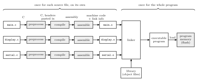
Figure 1: How a three-file C program becomes a running program. Each source file goes through the first three steps by itself. The preprocessor pastes in headers and expands macros, the compiler turns C into assembly, and the assembler turns assembly into an object file, which is machine code plus the information needed to link it. Only the linker sees the whole program. It joins the object files to each other and to the library members they use, fixes up every address, and writes one executable. That executable is then loaded into memory, which on the AVR means programming it into flash. Changing one source file means repeating the first three steps for that file alone, then linking again.
| Step | Takes | Produces | Notes |
|---|---|---|---|
| Preprocess | a .c file |
C with every #include pasted in and every macro expanded |
c-preprocessor-and-avr-headers |
| Compile | that C | assembly language | maps variables to memory, and translates each statement into instructions |
| Assemble | the assembly | an object file, .o |
assembly-process |
| Link | all the object files, plus the library | one executable | relocates and resolves addresses |
| Load | the executable | the program in memory, ready to run | on the AVR, the executable is programmed into flash |
Some compilers write machine code directly and never produce assembly text. The object file that comes out is the same either way, so the three middle steps are often just called “compiling”. In the simplified view the compiler itself does two things, mapping variables to memory and translating C into assembler instructions. Turning those instructions into machine code is the assembler’s work.
With the AVR GCC toolchain the object files and the executable are ELF files. The .hex file that gets programmed into flash is extracted from the ELF executable.
How a compiler maps variables to memory
The compiler decides where each variable goes by how long it has to exist.
| Declared | Lives | Stored | Address |
|---|---|---|---|
| outside every function: a global | for the whole run | in the fixed data area, which starts at the bottom of SRAM | fixed before the program runs |
| inside a function: a local | only while that call is running | in the call’s stack frame | depends on how deep the stack is at the call |
inside a function, marked static |
for the whole run, and it keeps its value between calls | with the globals | fixed |
nowhere: obtained from malloc() |
until it is given back | on the heap | handed out while the program runs |
Globals. A global can be used at any moment from any function, so it needs one address that never changes. The compiler reserves as many bytes as the type needs (c-language-basics), one variable after another, from the start of SRAM. On the ATmega324A that is 0x0100 = 256, because addresses 0 to 255 are taken by the registers and the I/O registers (memory-models). It is the same thing an assembly programmer does with .dseg and .byte.
Locals. A local exists only while its function is running, and a recursive function can have several calls running at once, each needing its own copy. So the compiler cannot give it a fixed address. Instead, each call builds a stack frame, a block on the stack holding that call’s arguments, its return address and its local variables. The return takes the frame away again (procedures-and-the-stack). The same local therefore sits at different addresses on different calls.
static locals. static inside a function keeps the name private to the function but gives the variable a global’s lifetime. It is stored with the globals, at a fixed address, and is never part of a frame. That is why it still holds its value the next time the function is called.
static on a global means something else. The variable is stored exactly like any global, but its name is private to its own source file. It is left out of the object file’s entry point table (below), so no other file can link to it.
The heap and the stack grow toward each other. The heap starts above the globals and grows toward higher addresses. The stack starts at the top of SRAM (RAMEND) and grows down. The free memory between them shrinks from both ends, and if the two meet, that is a stack overflow. Nothing on the chip detects it. The first sign is usually a global or heap variable changing for no reason.
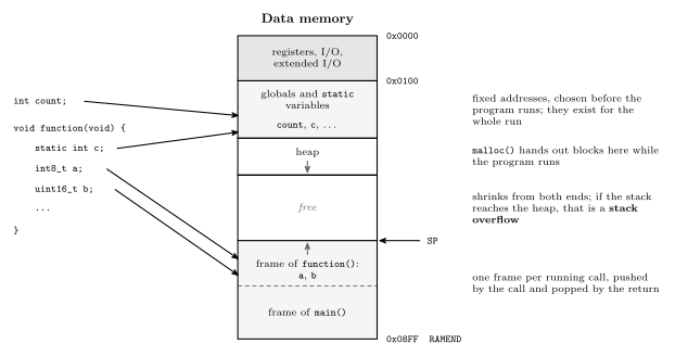
Figure 2: Where each kind of C variable ends up in the ATmega324A’s data memory, with the lowest address at the top. Globals and static variables are given fixed addresses from 0x0100, the first SRAM byte, so a static local such as c sits among the globals even though only its own function can name it. The heap, which malloc() hands out while the program runs, grows down the page toward the stack. The stack grows up the page from RAMEND. Each running call has a frame on it, and the frame of function() holds its locals a and b. When function() returns, that frame is gone. If the stack and the heap meet, the stack has overflowed.
Object files
A program of any size is split into several source files, and it pays to compile or assemble each one separately and then link them together. Change one file and only that file has to be compiled again. The others’ object files are reused as they are.
The price is that when a file is compiled, nobody knows where its code will end up. The file is translated as if it started at address 0. Every address inside it is relative to its own start, and any symbol defined in another file has no address at all yet. Once the linker has decided where everything goes, these addresses have to be fixed. A file that carries enough information for that fixing is a relocatable object module. “Object module” and “object file” mean the same thing.
So an object file is machine code plus information for the linker. There are many formats for it: a.out, COFF and ELF are object file formats, and DWARF is a format for debugging information, usually carried inside ELF files.
The six sections
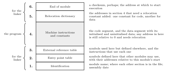
Figure 3: The six sections of a relocatable object module, numbered from the bottom. Only section 4 is program: the machine instructions and constants, assembled as if the module began at address 0. The other five are information for the linker. They say what the module is called and where its parts are in the file (1), which of its symbols other modules may use (2), which symbols it uses but does not define (3), which addresses in section 4 have to be moved when the module is moved (5), and where execution starts (6). Linking reads 1, 2, 3, 5 and 6 to decide how to rewrite 4.
1. Identification. The name of the module, where each of the other sections is in the file, and the date it was assembled.
2. Entry point table. The symbols defined in this module that other modules may refer to, with their values. A value is an address: a procedure’s entry point, or a variable’s location. It is relative to the beginning of this object module. A file that defines a procedure abs_value at its address 10 has the entry abs_value 10. Anything not listed, such as a static global or a label used only inside the module, cannot be reached from another file.
3. External reference table. The symbols used in this module but not defined in it, both procedure names and variables, and for each one the list of instructions that use it. Those instructions are the places the linker will have to fill in once it knows the address.
One module’s entry point is another module’s external reference. If module A defines SUM and module B calls it, SUM appears in A’s entry point table and in B’s external reference table.
4. Machine instructions and constants. The assembled code and constants: the code segment, and the data segment holding the initialised and the uninitialised data. An initialised global such as int n = 5; needs its starting value stored in the file. An uninitialised one needs only its size. The addresses used in this code are not yet correct. They were worked out as if the module started at 0, so they need relocation.
5. Relocation dictionary. The list of addresses in section 4 that need to be relocated. When the module is placed, a relocation constant is added to the instruction or data at each of those addresses. There is one constant for code and a different one for data, because a module’s code goes in program memory and its data in data memory, and the two start in different places.
6. End of module. Possibly a checksum, to catch a corrupted file, and the address at which execution starts.
The linker
The linker combines object modules, the program’s own and any it needs from libraries, into a single executable binary program of machine code.
Its problem is the assembler’s problem again, one level up. That is the external reference problem: symbols are used before their values are known. Module A can call a procedure in module B before the linker has even read B. So the linker, like the assembler, works in two passes (assembly-process).
Pass 1: lay the program out.
- Read each module’s sizes and give it a place, in link order. Each module’s code starts where the previous module’s code ended, and the same goes for data. These starting addresses are the module’s two relocation constants.
- Read every entry point table. Add each symbol to one global symbol table, with its final address: its value relative to its module, plus that module’s starting address.
Pass 2: copy and patch.
- Copy each module’s section 4 to its place.
- Relocate. For each address in the module’s relocation dictionary, add the module’s constant, the code constant for a code address and the data constant for a data address.
- Resolve. For each external reference, look the symbol up in the global table and write its final address into every instruction listed against it. A symbol that no module defines cannot be resolved, so linking fails with an “undefined reference” error.
The two words to keep straight:
Relocating = adding a constant: fixing an address that points into the module’s own code or data, which moved when the module moved. Resolving = finding the value of an external address: filling in an address that points into another module.
Where a module starts follows from the order alone. A module’s code starts at the program start plus the code sizes of every module linked before it, and its data starts at the data start plus the data sizes of those same modules. Code and data are counted separately, in their own units: on the AVR, words of program memory and bytes of data memory (memory-models).
Worked: linking four modules
Four object modules, each assembled from address 0. Their lengths are A = 400, B = 600, C = 500, D = 300. Each holds a branch within itself, a data move, and (apart from D) a call to the next module.
| Module | At | Instruction |
|---|---|---|
| A | 0 | BRANCH TO 200 |
| A | 200 | MOVE P TO X |
| A | 300 | CALL B |
| B | 0 | BRANCH TO 300 |
| B | 300 | MOVE Q TO X |
| B | 500 | CALL C |
| C | 0 | BRANCH TO 200 |
| C | 200 | MOVE R TO X |
| C | 400 | CALL D |
| D | 0 | BRANCH TO 200 |
| D | 200 | MOVE S TO X |
They are linked in the order A, B, C, D. The first 100 addresses hold start-up code, the code that runs before main (on the AVR it sets the stack pointer and prepares the data), so A starts at 100.
Pass 1: place the modules. Each starts where the previous one ends.
| Module | Length | Starts at | Ends at | Relocation constant |
|---|---|---|---|---|
| A | 400 | 100 | 499 | +100 |
| B | 600 | 100 + 400 = 500 | 1099 | +500 |
| C | 500 | 500 + 600 = 1100 | 1599 | +1100 |
| D | 300 | 1100 + 500 = 1600 | 1899 | +1600 |
The global symbol table holds the module names as entry points: A = 100, B = 500, C = 1100, D = 1600. The program ends at 1899, and 1900 is the first free address.
Pass 2: patch each instruction. An instruction moves to its offset plus its module’s start. A branch inside a module is relocated: the target moves by the same constant as the instruction, so it still lands on the same MOVE. A call to another module is resolved from the symbol table.
| New address | Was | Becomes | Because |
|---|---|---|---|
| 100 | A: BRANCH TO 200 |
BRANCH TO 300 |
relocate: 200 + 100 |
| 300 | A: MOVE P TO X |
MOVE P TO X |
no code address in it |
| 400 | A: CALL B |
CALL 500 |
resolve: B starts at 500 |
| 500 | B: BRANCH TO 300 |
BRANCH TO 800 |
relocate: 300 + 500 |
| 800 | B: MOVE Q TO X |
MOVE Q TO X |
no code address in it |
| 1000 | B: CALL C |
CALL 1100 |
resolve: C starts at 1100 |
| 1100 | C: BRANCH TO 200 |
BRANCH TO 1300 |
relocate: 200 + 1100 |
| 1300 | C: MOVE R TO X |
MOVE R TO X |
no code address in it |
| 1500 | C: CALL D |
CALL 1600 |
resolve: D starts at 1600 |
| 1600 | D: BRANCH TO 200 |
BRANCH TO 1800 |
relocate: 200 + 1600 |
| 1800 | D: MOVE S TO X |
MOVE S TO X |
no code address in it |
B’s constant, 500, is the start-up code plus all of A: 100 + 400. Every branch ends up pointing at the instruction it pointed at before: A’s branch at 100 reaches A’s MOVE at 300, and B’s at 500 reaches B’s MOVE at 800. The MOVEs name data, P, Q, R, S and X. Those addresses are fixed in the same way with each module’s data constant, which this example leaves out so that only the code is followed.
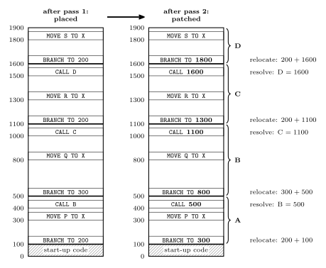
Figure 4: Linking four object modules in the order A, B, C, D, with addresses increasing up the page and start-up code in 0 to 99. Left: after the first pass. Every module has its place, each starting where the one before it ends, but the instructions are still exactly as assembled. A’s branch at 100 still names 200, its target counted from A’s own 0, and 200 is now in the middle of A, not at its MOVE. Each call still names a module, not an address. Right: after the second pass. Each branch within a module has been relocated by its module’s starting address, so it lands on that module’s MOVE again, and each call to another module has been resolved to that module’s start. The bold operands are the ones the linker rewrote.
Worked: where each module starts
Three modules have these sizes. Code is measured in words, because AVR program memory holds 16-bit words, and data in bytes.
| Module | Code size (words) | Data size (bytes) |
|---|---|---|
| 1 | 45 | 17 |
| 2 | 67 | 5 |
| 3 | 100 | 25 |
They are linked in the order 2, 1, 3, starting at program address 62 and data address 256. Where does each module’s code and data start, and where do two sample references inside module 1 end up?
Lay them out in link order, keeping a running total for each memory:
| Module | Code | Data | Code constant | Data constant |
|---|---|---|---|---|
| 2 | 62 to 62 + 67 − 1 = 128 | 256 to 256 + 5 − 1 = 260 | +62 | +256 |
| 1 | 129 to 129 + 45 − 1 = 173 | 261 to 261 + 17 − 1 = 277 | +129 | +261 |
| 3 | 174 to 174 + 100 − 1 = 273 | 278 to 278 + 25 − 1 = 302 | +174 | +278 |
The next free code word is 274 and the next free data byte is 303. Both totals come out the same as for any other order, because the same three sizes are added up. Only where each module falls changes.
Relocate inside module 1. Suppose module 1 has, at its own word 20, a branch to its own word 40, and at its own word 30, a load from its own data byte 4.
- The branch moves to 20 + 129 = 149, and its target is relocated by the same code constant, 40 + 129 = 169.
- The load moves to 30 + 129 = 159, and its operand is a data address, relocated by the data constant: 4 + 261 = 265.
Adding the code constant to the data address would give 133, and the load would read the wrong byte. This is why the relocation dictionary has to say whether each entry is a code address or a data address.
Why 62 and 256? On the ATmega324A, program words 0 to 61 (0x0000 to 0x003D) are the interrupt vector table (avr-interrupts), so 0x003E = 62 is the first free word. Data addresses 0 to 255 are registers and I/O, so 0x0100 = 256 is the first byte of SRAM.
Libraries
A library is a collection of object files with an additional index. It provides useful functions and procedures that have already been written, tested and compiled. The rule is not to reinvent the wheel: use library code where it exists.
The index maps each symbol to the member object file that defines it. When an external reference is still unresolved, say a call to printf, the linker looks the name up in the index, takes that one member, and links it in like any other module. The rest of the library stays out of the program.
The standard C library is the one every C program can count on. It covers:
- standard input and output (
stdio.h:printf,getchar, …) - string handling (
string.h:strlen,strcpy, …) - date and time functions (
time.h) - general utilities (
stdlib.h:malloc,abs,atoi, …)
On the AVR it is provided by avr-libc, which also supplies the avr/io.h and avr/interrupt.h headers.
Header files are not the library
The two are easy to mix up, because #include <stdio.h> is what lets a program call printf.
A header file (.h)
- defines useful preprocessor macros,
- declares the functions that are in the library, as function prototypes, and
- declares variables that are available externally, with
extern.
The library is the collection of object files that implement those functions.
A declaration says what a name is and what type it has, so the compiler can check every use and generate the call. It contains no code, so the call still has nowhere to go. The header is therefore read by the compiler, and the library is read by the linker. Each kind of mistake shows up at its own step:
| Missing | When it shows | Typical message |
|---|---|---|
| the header | compiling | implicit declaration of function printf |
| the library, or the file that defines the function | linking | undefined reference to printf |
How a header gets pasted in is covered in c-preprocessor-and-avr-headers.
Static and dynamic linking
Everything so far is static linking. All the object code, the library’s and the main program’s, is joined into one binary before the program ever runs.
In dynamic linking, linking happens at run time instead: a library procedure is linked when it is first called. The executable holds only a reference to it, and the library stays in a separate file that is loaded when the program needs it. DLLs (dynamic-link libraries) on Windows work this way, and so do shared libraries (.so files) on Linux.
| Static | Dynamic | |
|---|---|---|
| Library code is joined in | when the program is linked | when the procedure is first called |
| Library code is stored | inside every executable that uses it | once, in its own file, shared |
| Executable size | larger | smaller |
| Updating the library | means relinking each program | takes effect in every program at once |
Its advantages:
- It saves space. Libraries are not linked into the executable, so ten programs that use the same library share one copy of it.
- The library can be updated independently of the programs that use it. A bug fixed in the DLL is fixed in all of them, without relinking anything.
The second advantage is also its weakness. A program tested with one version of a library can break when another installation replaces that library with a version that behaves differently. On earlier versions of Windows this was common enough to be called “DLL hell”.
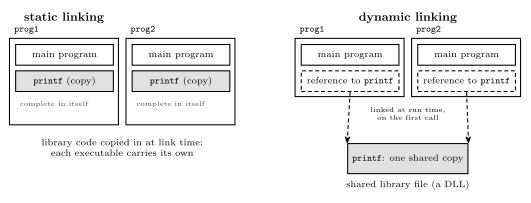
Figure 5: The same two programs, both calling printf, linked statically and dynamically. Static linking copies printf’s object code into each executable when it is linked, so each program carries its own copy and is complete in itself. Dynamic linking leaves a reference in each executable and keeps a single copy of printf in a shared library file. The reference is linked to that copy at run time, when printf is first called. That saves space, and updating the shared file changes the printf both programs get, for better or worse.
The ATmega324A has no operating system to load a library at run time, so every AVR program is linked statically. Everything it will ever call is already in flash.
Common mistakes
- Treating the header as the library.
#include <math.h>makessqrtcompile. It does not supplysqrt. Without the library the link fails with an undefined reference. - Counting from the wrong module. A module’s start depends on the modules linked before it in link order, not on its number. In the order 3, 2, 1, module 2 starts after module 3.
- Mixing code and data sizes. The code start adds up code sizes only, and the data start adds up data sizes only. On the AVR they are not even in the same unit: words against bytes.
- Off by one at a boundary. A module of size \(n\) starting at \(s\) occupies \(s\) to \(s + n - 1\), and the next module starts at \(s + n\).
- Relocating an external reference. A call into another module is not fixed by adding this module’s constant. Its address comes from the symbol table, which holds the other module’s start plus the symbol’s offset in it.
- Relocating a data address with the code constant, or the other way round.
- Expecting a local variable to keep its value between calls. The frame is gone when the function returns. Use
staticif the value must persist. - Returning a pointer to a local. The address points into a frame that no longer exists, and the next call will overwrite it.
- Thinking “interpreted” means “never compiled”. Java is compiled, to bytecode, and a JIT compiles parts of it again to machine code. What makes it interpreted is that the virtual machine, and not the processor, runs the bytecode.
See also
- assembly-process — the assembler’s two passes and symbol table, the same problem one level down
- c-preprocessor-and-avr-headers —
#include, macros, and the header against the library - procedures-and-the-stack — stack frames,
callandret, and where locals live - c-language-basics — declarations and how much memory each type takes
- memory-models · avr-architecture — the AVR’s word-addressed program memory and byte-addressed data memory
- avr-interrupts — the vector table that the program code follows
- instruction-set-architecture · 2026-09-07-introduction-to-embedded-c-programming — compiling one-to-many against assembling one-to-one
- fetch-decode-execute-cycle — what “runs on the processor” means
- 2026-10-15-compilation-and-linking — Lecture 22