State Machines
A state machine — equivalently a finite state machine (FSM) — is another name for a sequential circuit, viewed in terms of the states it can be in rather than the gates and flip-flops that implement it. See sequential-circuits for the circuit-level view and flip-flops-and-latches for the storage elements the state lives in.
What a state machine is
A state machine has:
- a finite number of possible states — \(N\) flip-flops give at most \(2^N\) of them;
- only one current state at any moment;
- the ability to transition to other states, based on the inputs and the current state.
The state is exactly the value held in the flip-flops (see sequential-circuits), so the flip-flop count bounds the state count. It does not fix it: how many flip-flops a given number of states actually costs is an encoding choice, made at the state-encoding step below.
Naming the two blocks of logic
The standard sequential-circuit structure has one combinational block computing two different things, and it is worth naming them separately:
\[\text{OUT} = g(\text{IN}, Q) \qquad\qquad D = f(\text{IN}, Q)\]
- \(Q\) is the present state (PS) — what the flip-flops hold right now.
- \(D\) is the next state (NS) — what they will hold after the next clock edge.
- \(g\) is the output logic; \(f\) is the transition logic (also called next-state logic).
Designing an FSM comes down to finding Boolean expressions for \(f\) and \(g\).
Defining the states from the problem
States are not handed to you — they come from the problem, and the useful question is what does the circuit need to remember?
Vending machine. A machine accepts 5c and 10c coins and dispenses a candy when it has received 15 cents in total. What are the states?
What the machine must remember is the running total inserted so far:
| Total inserted | 0 | 5 | 10 | 15 | 20 | 50 |
|---|---|---|---|---|---|---|
| Dispense candy? | no | no | no | yes | yes, plus change | — |
So the states are the totals 0, 5 and 10, with 15 and 20 being the ones that dispense (20 arises from inserting 10c on top of 10c, and needs change). A total of 50 is not a state at all: with only 5c and 10c coins the machine dispenses and resets long before it could get there, so it is unreachable.
Moore and Mealy machines
There are two types, differing only in what the output logic is allowed to see:
- Mealy machine — outputs depend on the current state and the inputs.
- Moore machine — outputs depend only on the current state (the flip-flop values). Consequently, outputs can only change when the state changes.
A Moore machine is a special case of a Mealy machine — the one where the output logic simply ignores its input connections. CSSE2010 sticks to Moore machines.
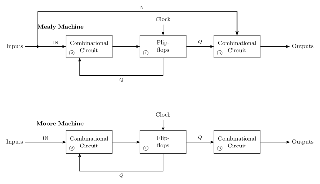
Figure 1: Mealy (top) and Moore (bottom). ① is the state, held in the flip-flops; ② is the transition logic; ③ is the output logic. The only structural difference is the branch drawn in bold: in a Mealy machine the inputs reach the output logic directly, so the outputs are a function of IN and Q; in a Moore machine the output logic sees Q alone.
State diagram notation
A state diagram draws the states as circles and the transitions as labelled arrows.
States are drawn as a circle split in two: the state name on top, the output value(s) underneath. So \(S_0\) over \(101\) is a state called \(S_0\) whose outputs are 101; the name is arbitrary and need not be \(S_n\) (a state called Alex over \(01\) is just as legal).
Transitions are arrows labelled with a logic expression over the inputs — if the expression is true, that transition is taken. Examples of labels: \(Z\), \(\overline{\text{RESET}}\), \(A + B\cdot\overline{C}\).
Two conventions worth knowing:
- No label means “true” — the transition is always taken on the next clock edge. This is what the arrows in a plain counter’s diagram look like.
- With only one input, the label may be written as just
0or1instead of a Boolean expression. This is a special case of the general form; \(1\) means the same as \(Z\) and \(0\) the same as \(\overline{Z}\).
Completeness
Each possible combination of inputs should be addressed exactly once for each state.
That is, the transition arrows leaving each state must encompass all possibilities, without overlap and without gaps. With \(N\) inputs there are \(2^N\) input combinations, so every state needs \(2^N\) transitions accounted for — though several combinations leading to the same next state can be merged onto one arrow with an OR’d label.
This is a checkable property, and checking it is the cheapest way to catch a half-finished design: if the labels on the arrows out of a state do not OR together to 1, some input combination has no defined behaviour; if any two of them can be true at once, the machine is ambiguous.
A counter is a state machine with no inputs
The design method for counters — write the sequence as a present-state/next-state table, read each \(D\) column off as a Boolean function of the \(Q\)’s, draw the gates — is steps 3, 5 and 6 of the pipeline below, applied to the degenerate case where the machine has no external inputs at all. A counter may or may not have external inputs.
Three things collapse when \(\text{IN}\) is empty:
- Transition logic. \(D = f(\text{IN}, Q)\) becomes \(D = f(Q)\), so the state table needs no input column and the excitation equations are functions of the \(Q\)’s alone.
- Output logic. A counter’s output is its state, so \(g\) is the identity and there is no second block of gates. That also makes every counter trivially a Moore machine.
- Completeness. With \(N = 0\) inputs there are \(2^0 = 1\) input combinations, so the completeness rule reduces to exactly one arrow out of each state — and by the “no label means true” convention, that arrow is unlabelled.
The state encoding step also disappears, or rather it is made for you: the states of a counter are already bit patterns, and the sequence you were given is the encoding.
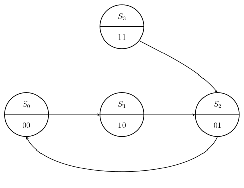
Figure 2: The 2-bit counter for \(00 \to 10 \to 01 \to 00\) drawn as a state diagram. Every arrow is unlabelled because the machine has no inputs, so each transition is taken unconditionally on the next clock edge; each state’s output half carries the count value, since a counter’s output is its state. \(S_3\) is the unused state: three states cannot fill a two-flip-flop machine, so its next state is a don’t-care, and choosing \(11 \to 01\) for it is what makes the design self-correcting.
Figure 2 read as a state table, with the unused row carrying the don’t-cares:
| Current state | Next state | \(Q_1\) | \(Q_0\) |
|---|---|---|---|
| \(S_0\) | \(S_1\) | 0 | 0 |
| \(S_1\) | \(S_2\) | 1 | 0 |
| \(S_2\) | \(S_0\) | 0 | 1 |
| \(S_3\) | (don’t care) | 1 | 1 |
The unused state is where the FSM framing pays for itself. A don’t-care is a free choice of transition, not an absence of one: the circuit will do something in state \(S_3\), and the only question is whether the arrow you have implicitly drawn leads back into the cycle or loops onto itself. An arrow from \(S_3\) to itself is a trap state — the machine leaves the intended cycle and never returns. There are two candidate simplifications for \(D_1\). The tidier one, \(D_1 = \overline{Q_1 \oplus Q_0}\), puts a self-loop on \(S_3\) and is rejected. The other sends \(11 \to 01\), back into the cycle, and is the robust design. See counters and 2026-08-17-counters for that working.
State tables
The same information as a state diagram, in tabular form. Two layouts, both in use.
One-dimensional — one row for every combination of state and inputs:
| Current State | Input \(U\) | Next State | \(Q_1\) | \(Q_0\) |
|---|---|---|---|---|
| \(S_0\) | 0 | \(S_3\) | 0 | 0 |
| \(S_0\) | 1 | \(S_1\) | 0 | 0 |
| \(S_1\) | 0 | \(S_0\) | 0 | 1 |
| \(S_1\) | 1 | \(S_2\) | 0 | 1 |
| \(S_2\) | 0 | \(S_1\) | 1 | 0 |
| \(S_2\) | 1 | \(S_3\) | 1 | 0 |
| \(S_3\) | 0 | \(S_2\) | 1 | 1 |
| \(S_3\) | 1 | \(S_0\) | 1 | 1 |
Two-dimensional — one row per state, with a next-state column for every combination of inputs:
| Current State | Next State (\(\overline{U}\)) | Next State (\(U\)) | \(Q_1\) | \(Q_0\) |
|---|---|---|---|---|
| \(S_0\) | \(S_3\) | \(S_1\) | 0 | 0 |
| \(S_1\) | \(S_0\) | \(S_2\) | 0 | 1 |
| \(S_2\) | \(S_1\) | \(S_3\) | 1 | 0 |
| \(S_3\) | \(S_2\) | \(S_0\) | 1 | 1 |
Both describe the same machine (a 2-bit up/down counter, \(U = 1\) counts up). The 2D form is more compact and makes completeness visually obvious — every input combination is a column, so a missing case is a missing column. The 1D form grows as \(2^N \times\) (number of states) but maps directly onto a truth table, which is what the next design step needs. In a Moore machine the output columns depend only on the current state, which is why they can sit in a per-state row at all.
State encoding
Each state must be encoded into flip-flop values before the design can become a circuit. Two choices to make:
- the number of flip-flops, and
- the bit patterns representing each state.
Ideally, choose the encoding that makes the combinational logic simple — for both the output logic and the next-state logic. Different encodings of the same machine give genuinely different gate counts.
Three common schemes, on a four-state machine:
| State | Binary | Gray | One-hot |
|---|---|---|---|
| \(S_0\) | 00 | 00 | 0001 |
| \(S_1\) | 01 | 01 | 0010 |
| \(S_2\) | 10 | 11 | 0100 |
| \(S_3\) | 11 | 10 | 1000 |
- Binary — the obvious count; \(\lceil \log_2 n \rceil\) flip-flops for \(n\) states.
- Gray — same width, but consecutive states differ in exactly one bit (see binary-number-representations).
- One-hot — one flip-flop per state, with only one flip-flop holding 1 at any time. Far more flip-flops, but the next-state and output logic often collapses to almost nothing, since “am I in state \(S_k\)” is just a single flip-flop’s output rather than a decoded combination.
Steps involved in FSM design
- Defining state based on the problem definition.
- Drawing the state diagram.
- Completing the state table (1D or 2D).
- State encoding, and re-doing the state table with encoded states.
- Obtaining the Boolean expressions for the next-state logic (i.e. the \(D\)’s) and for the outputs.
- Drawing the logic diagram.
- Simulating in Logisim to verify functionality.
- Building and testing the circuit in hardware.
Steps 1–6 are the pen-and-paper design; steps 7–8 are what the learning labs do with it. Steps 5 and 6 are the same techniques used to build a counter by hand — see counters and circuit-schematics.
See also
- sequential-circuits · flip-flops-and-latches · counters · shift-registers
- 2026-08-17-counters — Lecture 7, where this design method is first used (on counters)
- 2026-08-20-state-machines — Lecture 8
- week9-lab-avr-interrupts — Lab 14: a stopwatch controller designed as a Moore machine and written in C