Lecture 8 — State Machines
See state-machines for the reference material — Moore vs Mealy, the diagram and table notation, encoding schemes and the design procedure — and sequential-circuits, flip-flops-and-latches and counters for the background. The drawing conventions for state diagrams and state tables are catalogued in csse2010-diagram-notation.
Outline
- State diagrams
- State tables
- State encoding
Sequential circuits
- State = the value stored in the flip-flops.
- Output depends on the input and the state.
- Next state depends on the inputs and the state.
In the block diagram, the combinational circuit is the logic gates:
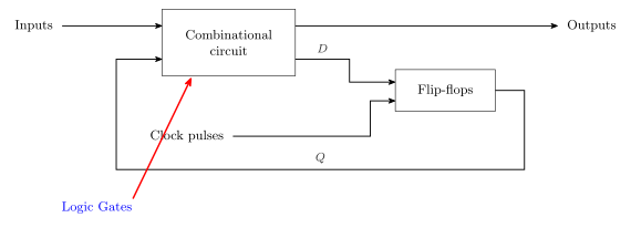
Figure 1: The sequential-circuit block diagram (from Mano, Digital Design, 3rd ed.). Flow is left to right with the state fed back around the outside, and the clock enters on its own stub reaching only the flip-flops — never the gates. The red arrow and the blue Logic Gates label mark the combinational circuit as the logic gates. D and Q name the two feedback-side wires, which is what makes the two functions below readable off the picture.
Writing \(Q\) for the present state (PS) and \(D\) for the next state (NS), the one box marked Combinational circuit is really two functions computed side by side:
\[\underbrace{\text{OUT} = g(\text{IN}, Q)}_{\text{output logic}} \qquad\qquad \underbrace{D = f(\text{IN}, Q)}_{\text{transition logic}}\]
The clock pulses reach only the flip-flops, never the gates — see sequential-circuits.
“Output depends on input and state” is the general sequential-circuit statement, i.e. the Mealy form. A Moore machine is narrower: the output depends on the state alone. Every state machine drawn in this course from here on obeys the narrower rule.
State machines
Sequential circuits can also be called state machines, or finite state machines (FSMs). A state machine has a finite number of possible states, is in only one current state at a time, and can transition to other states based on the inputs and the current state.
\(N\) flip-flops give \(2^N\) states.
Defining the states from the problem
The first step in a design is not a circuit at all — it is deciding what the states are:
A vending machine accepts 5 cent and 10 cent coins, and dispenses a candy when it receives 15 cents in total. What can be the different states?
Tabulate the running total:
| Coins inserted | 0 | 5 | 10 | 15 | 20 | 50 |
|---|---|---|---|---|---|---|
| Candy? | ✗ | ✗ | ✗ | ✓ | ✓ + change | — |
So the states are the amounts accumulated so far. 15 dispenses; 20 dispenses and owes change (reachable by putting 10c on top of 10c). 50 is ruled out — with only 5c and 10c coins the machine dispenses long before it could accumulate that much, so it is not a reachable state.
The transferable move: ask what must the circuit remember?, and the answer is the state set.
Moore vs Mealy
- Mealy — outputs depend on the current state and the inputs.
- Moore — outputs depend only on the current state (the flip-flop values), so outputs can only change when the state changes.
A Moore machine is a special case of a Mealy machine, and this course sticks to Moore machines.
The two structures have the same three-block shape: combinational circuit → flip-flops → combinational circuit, with the state fed back to the first block. The only difference is one branch — in the Mealy machine the input line also runs forward into the second (output) combinational block; in the Moore machine it does not. Both are drawn in the “Moore and Mealy machines” section of state-machines.
State diagrams
The notation for a state diagram:
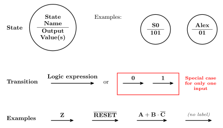
Figure 2: The state-diagram notation. A state is a circle split by a horizontal chord: state name above, output value(s) below. State names are free-form — a systematic S0 and an arbitrary word (Alex) are both allowed — and outputs are a bare bit string with no separators. A transition is a plain single-headed arrow labelled with a Boolean expression written above it; the red box marks the special case where a machine has exactly one input and the label degenerates to a bare 0 or 1. The bottom row gives example labels, including the unlabelled arrow, which means true.
Reading it off:
- A state is a circle divided by a horizontal chord — state name above, output value(s) below. Nothing else goes inside.
- Names are free-form. \(S_0\), \(S_1\), … is a convention, not a rule;
Alexis just as legal. - A transition is an arrow labelled with a logic expression. If the expression is true, the transition is made. Label algebra is the ordinary Boolean notation of boolean-algebra: overbar for NOT,
·or juxtaposition for AND,+for OR. - No label means “true” — i.e. always transition.
- Exactly one input is a special case: the label may be written as a bare
0or1rather than \(\overline{Z}\) or \(Z\). This is the red-boxed case in the figure.
The notation leaves two things unsettled — see csse2010-diagram-notation:
- how to mark the start / reset state (the diagrams below mark none: no incoming stub, no double circle, no
resetlabel), and - how to draw a self-loop (there is no set shape for one, although the completeness rule below guarantees most machines need them).
Worked: a two-state lock system
A lock with one input key and one output locked:
IN key |
OUT locked |
|---|---|
| 0 | 1 |
| 1 | 0 |
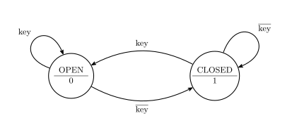
Figure 3: The two-state lock. The state name sits above the chord and the output value below it, so OPEN is the state whose locked output is 0. With one input there are two arrows out of every state, and here they account for both values of key: present the key and the lock opens or stays open, remove it and it closes or stays closed. The self-loops are needed for completeness.
Example — binary counter with 2-bit output
A counter has no inputs at all beyond the clock, so every arrow is unlabelled — the machine advances one state per clock edge regardless.
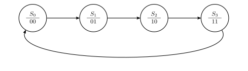
Figure 4: A 2-bit binary counter as a state machine: the four states in a left-to-right row, forward transitions between neighbours, and the wrap-around drawn as a long arc below the row. Outputs 00, 01, 10, 11, and no transition labels because there is no input to test. No state is marked as the start state. Compare the gate-level construction of the same thing in the counters note.
Example — binary up/down counter, one input
One input \(U\): 1 means count up, 0 means count down. The two output sequences:
| \(U = 1\) | 00, 01, 10, 11, 00, 01, … |
|---|---|
| \(U = 0\) | 11, 10, 01, 00, 11, 10, … |
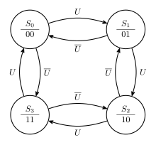
Figure 5: The up/down counter with a single input. Each state has exactly two arrows out — one for U and one for its complement — which is completeness for a one-input machine. The U arrows run clockwise through the ring and the U-bar arrows run anticlockwise. The states sit in a square ring because a straight row does not extend to a machine with arrows running both ways.
Because there is exactly one input, the one-input special case applies: these labels could equally be written as bare 1 and 0.
Example — binary up/down counter, two inputs
Two inputs \(U\) and \(D\), giving four commands:
| \(U\) | \(D\) | Meaning |
|---|---|---|
| 1 | 0 | count up |
| 0 | 1 | count down |
| 1 | 1 | set to 11 |
| 0 | 0 | reset to 00 |
With \(N\) inputs there are \(2^N\) transitions to account for out of each present state — here \(2^2 = 4\) arrows out of every state. Working the four commands through each state gives:
| Current state | \(U\overline{D}\) (up) | \(\overline{U}D\) (down) | \(UD\) (set 11) | \(\overline{U}\,\overline{D}\) (reset 00) |
|---|---|---|---|---|
| \(S_0\) (00) | \(S_1\) | \(S_3\) | \(S_3\) | \(S_0\) |
| \(S_1\) (01) | \(S_2\) | \(S_0\) | \(S_3\) | \(S_0\) |
| \(S_2\) (10) | \(S_3\) | \(S_1\) | \(S_3\) | \(S_0\) |
| \(S_3\) (11) | \(S_0\) | \(S_2\) | \(S_3\) | \(S_0\) |
Combinations sharing a destination merge onto one arrow, and the merged labels simplify:
| Transition | Merged label | Simplifies to |
|---|---|---|
| \(S_0 \to S_3\) | \(\overline{U}D + UD = D(\overline{U} + U)\) | \(D\) |
| \(S_1 \to S_0\) | \(\overline{U}D + \overline{U}\,\overline{D} = \overline{U}(D + \overline{D})\) | \(\overline{U}\) |
| \(S_2 \to S_3\) | \(U\overline{D} + UD = U(\overline{D} + D)\) | \(U\) |
| \(S_3 \to S_0\) | \(U\overline{D} + \overline{U}\,\overline{D} = \overline{D}(U + \overline{U})\) | \(\overline{D}\) |
Both steps are the complement law \(X + \overline{X} = 1\) used once each — see boolean-algebra.
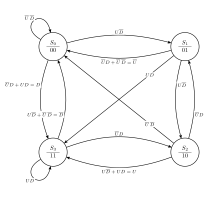
Figure 6: The up/down counter with set and reset. Every state has four input combinations to account for, drawn here as three arrows each once the combinations sharing a destination are merged. S0 keeps its reset combination as a self-loop and S3 keeps its set combination as one; the labels are shown in merged form with the simplification after the equals sign.
Completeness
Each possible combination of inputs should be addressed exactly once for each state — i.e. transition arrows from each state must encompass all possibilities (exactly once).
The two-input counter above is the check in practice: four input combinations, four accounted for out of every state, none twice. Equivalently — the labels leaving a state must OR to 1 (no gap) and no two of them can be true at once (no ambiguity).
State tables
A state diagram can equivalently be written as a state table. There are two forms; both here are filled in for the up/down counter with the single input \(U\) (1 up, 0 down) — the machine of Figure 5.
One-dimensional — a row for every combination of state and inputs:
| Current State | Input \(U\) | Next State | \(Q_1\) | \(Q_0\) |
|---|---|---|---|---|
| \(S_0\) | 0 | \(S_3\) | 0 | 0 |
| \(S_0\) | 1 | \(S_1\) | 0 | 0 |
| \(S_1\) | 0 | \(S_0\) | 0 | 1 |
| \(S_1\) | 1 | \(S_2\) | 0 | 1 |
| \(S_2\) | 0 | \(S_1\) | 1 | 0 |
| \(S_2\) | 1 | \(S_3\) | 1 | 0 |
| \(S_3\) | 0 | \(S_2\) | 1 | 1 |
| \(S_3\) | 1 | \(S_0\) | 1 | 1 |
Two-dimensional — one row per state, with a next-state column for every combination of inputs:
| Current State | Next State (\(\overline{U}\)) | Next State (\(U\)) | \(Q_1\) | \(Q_0\) |
|---|---|---|---|---|
| \(S_0\) | \(S_3\) | \(S_1\) | 0 | 0 |
| \(S_1\) | \(S_0\) | \(S_2\) | 0 | 1 |
| \(S_2\) | \(S_1\) | \(S_3\) | 1 | 0 |
| \(S_3\) | \(S_2\) | \(S_0\) | 1 | 1 |
In the full layout the last two columns sit under a single spanning Outputs header, and the \(\overline{U}\) / \(U\) columns under a spanning Next State header; the tables above repeat the header text instead. Two smaller notational points, both unresolved in csse2010-diagram-notation: the output bits are written both unsubscripted (Q1, Q0) and subscripted (\(Q_1\), \(Q_0\)), and the first column is headed both Current State and Present State. Nothing in the course picks a winner, so the subscripted form is used here for consistency with the rest of these notes.
The output columns repeat in the 1D form (both rows for \(S_0\) output 00) because this is a Moore machine — the output is a property of the state alone, which is exactly why the 2D form can give it one column per state. In a Mealy machine the 2D form’s output would have to be split by input as well.
State encoding
Each state must be encoded into flip-flop values: choose the number of flip-flops and the bit patterns representing each state. Ideally, pick the encoding that makes the combinational logic simple — for both the output logic and the next-state logic.
Two encodings of the four-state binary counter:
| State | Binary | One-hot |
|---|---|---|
| \(S_0\) | 00 | 0001 |
| \(S_1\) | 01 | 0010 |
| \(S_2\) | 10 | 0100 |
| \(S_3\) | 11 | 1000 |
One-hot coding uses one flip-flop per state, with only one flip-flop holding 1 at any time — four flip-flops here instead of two. A third scheme, Gray coding, is in state-machines.
Worked: one-hot encoding of the binary counter with 2-bit output
Call the four flip-flops \(F_3 F_2 F_1 F_0\), one per state, with state \(S_k\) encoded by \(F_k = 1\). The counter’s cycle \(S_0 \to S_1 \to S_2 \to S_3 \to S_0\) becomes
\[D_1 = F_0, \qquad D_2 = F_1, \qquad D_3 = F_2, \qquad D_0 = F_3\]
— i.e. no next-state gates at all, just four wires. That circuit is a 4-bit shift register wired end to end, otherwise known as a ring counter (see shift-registers and counters).
The outputs are no longer free, though. \(Q_1\) is 1 in \(S_2\) and \(S_3\), and \(Q_0\) is 1 in \(S_1\) and \(S_3\):
\[Q_1 = F_2 + F_3, \qquad Q_0 = F_1 + F_3\]
so two OR gates. Under binary encoding the trade runs the other way: the outputs are the flip-flops (\(Q_1, Q_0\) straight out, no gates) but the next-state logic needs \(D_1 = Q_1 \oplus Q_0\) and \(D_0 = \overline{Q_0}\). That is the point of choosing an encoding, in miniature — the encoding decides where the gates end up, and how many flip-flops you pay for.
Sequence detector example
Design a state machine which detects the pattern 101 in an incoming bit stream and outputs a 1 whenever it detects this pattern. The output is 1 for one clock cycle after the third digit is clocked in.
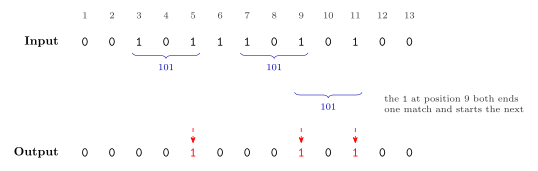
Figure 7: A worked bit stream for the 101 detector. The numbers along the top are bit positions. The braces mark the three occurrences of 101 in the input; the third is drawn on its own level because it overlaps the second. The dashed arrows show which output bit each match raises, and those output bits are red.
Three detections: the 101 finishing at position 5, the one finishing at position 9, and the overlapping one finishing at position 11 — the 1 at position 9 serves as both the end of one match and the start of the next. That is the whole difficulty of the problem: after a successful detection the machine must not go back to “seen nothing”, because it has already seen the first 1 of a possible next match.
The machine itself is one of the two examples worked through in the Blackboard recordings.
Steps involved in FSM design
- Defining state based on the problem definition.
- Drawing the state diagram.
- Completing the state table (1D or 2D).
- State encoding and re-doing the state table with encoded states.
- Obtaining the Boolean expressions for next state logic (i.e. the \(D\)’s) and for outputs.
- Drawing the logic diagram.
- Simulating in Logisim to verify functionality. ⎫ the labs
- Building and testing the circuit in hardware. ⎭
Steps 1–6 are lecture material; 7 and 8 are what the learning labs do — see week5-lab-state-machines. Steps 5 and 6 are the same derivation used to build a counter by hand — see counters and circuit-schematics.
The examples above take the up/down counter to step 3 and the plain counter to step 4; steps 5 and 6 are exercised on the sequence detector in the recordings.
Two recordings on Blackboard work through further examples, and should be watched after this lecture.
See also
- state-machines · sequential-circuits · flip-flops-and-latches · counters · shift-registers
- csse2010-diagram-notation — the state-diagram and state-table conventions
- week5-lab-state-machines — Lab 8, which is steps 7–8 of the procedure above
- 2026-08-17-counters — Lecture 7