Lecture 24 — Memory, Disks and Files
The memories a computer is built from, from the registers down to the disk, and how a disk’s sectors become named files. The note covers why computers need memory and the ways memory is classified; static and dynamic RAM; volatile and non-volatile memory and the family from ROM to flash; the ATmega324A’s three memories; when a megabyte is not a megabyte; the generations of DRAM; the memory hierarchy and cache; how a magnetic disk is organised and how long it takes to reach a sector; and files, file systems, formatting, blocks and fragmentation. The reference notes are memory-technologies, memory-hierarchy-and-cache, magnetic-disks and file-systems. The AVR’s address spaces are in memory-models.
Goals
- Classify a memory as random or sequential access, static or dynamic, volatile or non-volatile, read-only or read/write, and primary or secondary, and place SRAM, DRAM, ROM, flash, SSDs and hard disks on each axis.
- Explain how SRAM and DRAM store a bit, and why DRAM needs refreshing.
- Tell ROM, EPROM, EEPROM and flash apart by how each is erased, and say which memory on the ATmega324A holds what.
- Convert between the decimal and binary meanings of kB, MB and GB, and say which is used where.
- Describe the memory hierarchy and explain how a cache reduces the average access time.
- Describe a disk’s platters, surfaces, tracks, sectors and cylinders, and calculate its average access time.
- Explain what a file system does, what formatting and deleting change, how block size trades map size against wasted space, and why fragmentation slows access.
Why computers need memory
A computer needs memory for three different jobs. A running program needs somewhere to keep its temporary results. The program itself has to be stored somewhere the processor can fetch it from. And some things, settings above all, have to be remembered while the power is off.
They pull in different directions: fast and endlessly rewritable for the first, permanent for the third. So there are many different types of memory, and five questions sort them (memory-technologies).
Classifying memory
| Axis | Meaning | Examples |
|---|---|---|
| Random access or sequential access | any cell reached directly by its address, or the data passed over in order to get to it | almost all memory chips are random access; a tape is sequential |
| Static or dynamic | a bit held by a flip-flop, or as charge that must be refreshed | SRAM (flip-flops) is static; DRAM is dynamic |
| Volatile or non-volatile | contents lost or kept at power-off | SRAM and DRAM are volatile; flash is non-volatile |
| Read-only | cannot be written in normal use | ROM |
| Primary or secondary | addressed directly by the processor, or reached through I/O | SRAM (and DRAM) are primary; SSDs and HDDs are secondary |
Random access is what an address decoder provides (memory-models): the address bits select one cell directly, and every cell takes the same time. With 1 address bit there are 2 cells to choose from, with 2 bits 4, each address picking out its own cell.
Where SRAM, DRAM, ROM, flash, SSDs and hard disks fall on each of the five axes is charted in memory-technologies.
Static and dynamic memory
Static memory, SRAM, keeps each bit in a flip-flop or latch (flip-flops-and-latches). A flip-flop holds its bit for as long as there is power with nothing more to do, and it is fast, but it takes several transistors per bit, so SRAM is expensive.
Dynamic memory, DRAM, builds each cell from a transistor, used as a switch, and a capacitor. The bit is the charge on the capacitor. That charge leaks away, so every cell has to be refreshed, read and written back, every few tens of milliseconds (around 20 ms).
Both are kinds of RAM, random access memory. The name once meant only that any cell could be reached directly, as opposed to sequential access, which would make ROM random access too. In current use it means volatile read/write memory, and SRAM and DRAM are its two forms. The cells of each are drawn in memory-technologies.
Volatility
A volatile memory loses its contents when the power goes off, and both SRAM and DRAM are volatile. DRAM is the more forgetful of the two: even with the power on, a cell that is not refreshed loses its charge within milliseconds.
A non-volatile memory keeps its contents with the power off. ROM, EPROM, EEPROM and flash are all non-volatile, and they differ in whether, and how, they can be rewritten.
Non-volatile memory chips
The four non-volatile chips form a family, each easier to rewrite than the last.
- ROM (read-only memory) has its contents fixed in the silicon by the maker. It can never be changed.
- EPROM (erasable programmable ROM) is programmed electrically and erased with ultraviolet light. The package has a small window over the chip; a UV lamp shone through it erases the whole chip, ready to be programmed again.
- EEPROM (electrically erasable PROM) is erased by applying a voltage, so it can be rewritten in the circuit, one cell at a time.
- Flash is a newer EEPROM. The two began as different technologies and have been converging; what still separates them is that flash is written and erased in blocks, while EEPROM is written and erased one cell at a time.
The ATmega324A’s flash is split into two blocks, an application section and a boot loader section. A boot loader is a small program that writes a new program into the application section, and keeping the two in separate blocks lets one be erased and rewritten while the other is left alone. Other AVR devices have a single flash block, and some have more. The family is drawn in memory-technologies.
The ATmega324A’s memories
The chip’s block diagram has three memories among its peripherals, each a separate address space with its own assembler segment (memory-models):
| Memory | Technology | Volatile? | Holds | Segment |
|---|---|---|---|---|
| FLASH, 32 kB | flash | no | the program | .cseg |
| SRAM, 2 kB | static RAM | yes | variables and the stack | .dseg |
| EEPROM, 1 kB | EEPROM | no | data that must survive power-off | .eseg |
All three connect to the AVR CPU over the chip’s internal data bus, alongside the A/D converter, the analog comparator, SPI, TWI, JTAG and the four timer/counters. What each memory is for, and how the boot loader rewrites the application block, is drawn in memory-technologies; the address maps of program and data memory are in memory-models.
When is a megabyte not a megabyte?
A megabyte is not always \(2^{20}\) bytes: sometimes it is a million. In SI units and in physics, kilo, mega and giga are \(10^3 = 1000\), \(10^6\) and \(10^9\). In computing they have conventionally, or at least historically, been \(2^{10} = 1024\), \(2^{20}\) and \(2^{30}\). The full treatment is in memory-technologies.
Worked: 1 MB and 1 GB in their various meanings
How many bytes are in 1 MB, and in 1 GB? How big is the difference between the meanings?
1 MB.
- Conventionally: \(1\text{ MB} = 2^{10}\text{ kB} = 1{,}024\text{ kB} = 2^{20}\text{ B} = \mathbf{1{,}048{,}576}\) B.
- Sometimes: \(1\text{ MB} = 10^6\text{ B} = \mathbf{1{,}000{,}000}\) B.
- Or in between: \(1000\text{ kB} = 1000 \times 1024 = \mathbf{1{,}024{,}000}\) B.
1 GB.
- Conventionally: \(1\text{ GB} = 2^{10}\text{ MB} = 2^{20}\text{ kB} = 2^{30}\text{ B} = \mathbf{1{,}073{,}741{,}824}\) B.
- Sometimes: \(1\text{ GB} = 10^9\text{ B} = \mathbf{1{,}000{,}000{,}000}\) B.
- Or in between: \(1000 \times 2^{20} = \mathbf{1{,}048{,}576{,}000}\) B.
The difference. \(2^{30} - 10^9 = 73{,}741{,}824\) bytes, and
\[\frac{73{,}741{,}824}{10^9} = 7.37\,\% \approx 7.4\,\%.\]
So the binary gigabyte is 7.4 % bigger than the decimal one. (Measured the other way, the decimal gigabyte is \(73{,}741{,}824 / 2^{30} = 6.87\,\%\) smaller.) For the megabyte the gap is only \(48{,}576 / 10^6 = 4.86\,\%\), and for the kilobyte \(24/1000 = 2.4\,\%\): the gap grows with each prefix because each step multiplies by 1024 rather than 1000.
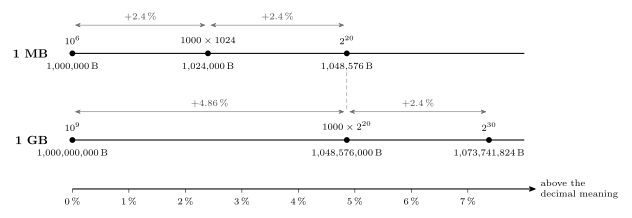
Figure 1: The three meanings of 1 MB and of 1 GB, placed on one scale by how far each lies above the decimal meaning. A binary megabyte, 1,048,576 bytes, is 4.86 per cent above a million bytes; a binary gigabyte, 1,073,741,824 bytes, is 7.37 per cent above a billion. The in-between meaning, a decimal thousand of the next binary unit down, is always one factor of 1.024 (2.4 per cent, the arrows) short of the binary one, so the in-between gigabyte lands exactly on the binary megabyte’s 4.86 per cent (dashed).
When do we use powers of 2, and when powers of 10?
- Main memory capacity is always quoted in powers of 2: \(1\text{ GB} = 1024 \times 1024 \times 1024\text{ bytes} = 2^{30}\) bytes. A memory with \(n\) address lines has exactly \(2^n\) cells (2 for one line, \(2^2 = 4\) for two, \(2^3 = 8\) for three), so memory comes in powers of 2.
- Hard disk makers quote powers of 10, \(1\text{ GB} = 1000 \times 1000 \times 1000\text{ bytes} = 10^9\) bytes, which makes a disk look bigger.
- Operating systems such as Windows count in powers of 2, which is why a new disk always shows less than its label.
- Data rates are usually powers of 10: 1 Gbps (gigabit per second) is \(10^9\) bits per second.
- Occasionally a figure mixes the two.
Worked: the 1.44 MB floppy disk
A “1.44 MB” floppy disk stores \(1.44 \times 1000 \times 1024\) bytes. How many bytes is that, and how many MB is it in each of the two pure meanings?
\[1.44 \times 1000 \times 1024 = \mathbf{1{,}474{,}560}\ \textbf{bytes}.\]
In binary megabytes that is \(1{,}474{,}560 / 2^{20} = 1.40625\) MB; in decimal megabytes, \(1{,}474{,}560 / 10^6 = 1.47456\) MB. The “1.44” is neither: it counts thousands of 1024-byte kilobytes, a decimal mega of binary kilos.
Worked: a disk in the operating system
A disk sold as 500 GB is formatted and the operating system, counting in powers of 2, reports its size. About how many “GB” does it show?
The maker’s 500 GB is \(500 \times 10^9\) bytes. The OS divides by \(2^{30}\): \(500 \times 10^9 / 1{,}073{,}741{,}824 = \mathbf{465.66}\) GB. Nothing is missing; the gigabytes differ by 7.4 %. (Formatting takes a little more, for the file system’s tables.)
Kibibytes and mebibytes
In SI units kilo, mega and giga mean powers of 10, so separate names were standardised for the binary meanings:
- 1 kibibyte \(=\) 1 KiB \(=\) 1024 bytes;
- 1 mebibyte \(=\) 1 MiB \(=\) 1024 KiB;
- 1 gibibyte \(=\) 1 GiB \(=\) 1024 MiB.
They have not caught on, and kilo, mega and giga are still used for both meanings. These notes do the same, so the context decides which is meant, and it is worth saying so when it matters.
Types of DRAM
DRAM stores bits as charge on capacitors rather than in flip-flops. Its cells are smaller, so a chip holds more bits than a static memory chip, at the cost of being slower. The cell has stayed the same while the interface has gone through many generations:
- Fast Page Mode (FPM DRAM) and Extended Data Out (EDO DRAM), a closely related pair of asynchronous designs, EDO a refinement of FPM;
- Synchronous DRAM (SDRAM), clocked, the step every later type builds on;
- Rambus DRAM (RDRAM);
- Double Data Rate DRAM (DDR DRAM), generations 1, 2, 3, 4 and now 5, which move data on both clock edges;
- and, for graphics cards, GDDR, now at GDDR7.
What each changed is in memory-technologies.
The memory hierarchy
No memory is fast, big and cheap at once, so computers use a hierarchy of them, with the CPU at the top.
| Level | Technology | Capacity | Cost per bit | Access time |
|---|---|---|---|---|
| Registers (r0 to r31 on the AVR) | flip-flops | under a kB | $$$ | ~1 ns |
| Cache, itself in levels L1, L2, L3 | SRAM | ~MB | $$ | ~10 ns |
| Main memory | DRAM | ~GB | $ | up to ~1 µs |
| Magnetic disk | HDD, or an SSD | ~TB | a fraction of a $ | ~1 to 10 ms |
| Tape, optical disk | ~PB | a smaller fraction | ~100 ms and up |
Going down the hierarchy, capacity increases, cost per bit falls, and access time grows. The values are orders of magnitude, and the point is the trend. The hierarchy is drawn as a pyramid, with the CPU at its apex, in memory-hierarchy-and-cache.
Cache memory
A CPU runs faster than its main memory can answer, and memory fast enough to keep up is too expensive to use for all of it. A CPU that waited on main memory for every access would spend most of its time idle.
A cache gets around this with a small amount of very fast memory in front of the large, slow one. It holds copies of the words in most frequent use. The CPU looks in the cache first and goes to main memory only if the word is not there, so when most accesses find their word in the cache, the average access time comes down close to the cache’s own.
Worked: why a loop runs from the cache
A program runs
for (i = 0; i < 1000; i++) { ... }, readingionce per iteration. The cache answers in 10 ns, main memory in 1 µs, and the CPU looks in the cache first. What fraction of the reads ofihit the cache, and what is their average access time?
The first read of i is a miss: i is fetched from main memory over the bus and a copy is kept in the cache. Every later read finds it there. So 999 of the 1000 reads hit, \(h = 0.999\), and
\[t_{\text{avg}} = t_c + (1 - h)\,t_m = 10 + 0.001 \times 1000 = \mathbf{11\ ns},\]
against 1000 ns with no cache. A loop that ran \(10^{20}\) times would make the single miss vanish entirely. Programs reuse the same few words like this all the time, which is why a small cache answers most accesses. The general formula, and the cases \(h\) = 90, 95 and 99 %, are in memory-hierarchy-and-cache.
Cache levels
A cache is often built in levels, each larger and a little slower than the one before. L1 is inside the CPU itself and runs at the CPU’s speed; it is small, typically 32 kB to 128 kB. L2 is bigger, typically 256 kB to 16 MB, and may be slightly slower than the CPU; it can be on the CPU’s own chip or on a separate chip, possibly in the same module. Some machines add an L3, typically 2 MB to 256 MB. The CPU tries L1, then L2, then L3, and only then main memory. These sizes are in bytes: B is a byte and b is a bit, so 32 kB is \(32 \times 1024 \times 8 = 262{,}144\) bits.
Magnetic disks
A hard disk drive (HDD) is a stack of platters with a magnetised coating, spinning together on one spindle at thousands of rpm, 10,000 rpm on a fast disk. Data is stored magnetically in circular tracks: a patch magnetised one way (north up) is a 1 and the other way (south up) a 0. The read/write heads float a few nanometres (of the order of 5 nm) above the surfaces, and both sides of each platter are usually used.
The simplified view
A disk with four platters has eight surfaces, numbered 0 to 7 from the bottom, and one read/write head per surface. The heads are on one arm assembly and move in and out together. The disk is drawn from the side, with the cylinder the heads sit over, in magnetic-disks.
Sectors, tracks and cylinders
A track is one circle on one surface, and each track is divided into sectors. A cylinder is the set of tracks at a given radial position. Assuming both sides of every platter are used,
\[\text{number of tracks in a cylinder} = 2 \times \text{number of platters},\]
so the four-platter disk has 8 tracks per cylinder. The heads move together, to a certain cylinder (magnetic-disks).
Sectors
Each track is cut into fixed-length sectors, and the sector is the smallest unit the disk handles: it always reads or writes a whole one. A sector starts with a preamble, a known pattern the head uses to synchronise to the data; then comes the data; then error correction codes (ECCs) to repair small read errors; and then an inter-sector gap before the next sector.
Laid along the track, that is PRE | DATA | ECC | GAP. It is the same pattern as a UART frame of start bit, data, parity and stop bits (serial-communication): something to synchronise on, the payload, a check, and a separator. The layout is drawn in magnetic-disks.
Worked: how much of a disk holds files
About 85 % of a disk’s capacity is usable by the operating system, and about 95 % of that is usable for user data; the remaining ~5 % is file-system overhead. What fraction of the raw capacity holds user data, and how much of a 1 TB (\(10^{12}\) byte) disk is that?
User data gets \(0.85 \times 0.95 = 0.8075\), about 81 % of the raw capacity; file-system overhead is \(0.85 \times 0.05 = 4.25\,\%\) of it. On a 1 TB disk: \(0.85 \times 10^{12} = 850\) GB for the OS, and \(0.8075 \times 10^{12} = \mathbf{807.5}\) GB for files, which an OS counting in powers of 2 shows as \(807.5 \times 10^9 / 2^{30} = 752.04\) GB.
Access time
\[\text{access time} = \text{seek time} + \text{rotational latency} + \text{transfer time}\]
The seek time is spent moving the heads to the right cylinder. The rotational latency is spent waiting for the sector to come round under the head. The transfer time is the sector passing under the head as it is read, and it is so short compared with the other two that it can be neglected.
Average seek time. Suppose seek time is proportional to the distance the heads move. Measure positions from 0 at one edge to 1 at the other, and take the start \(x\) and the target \(y\) as independent and uniformly random. The average distance is
\[\int_0^1\!\!\int_0^1 |x - y|\,dx\,dy = 2\int_0^1\!\!\int_0^x (x-y)\,dy\,dx = 2\int_0^1 \frac{x^2}{2}\,dx = \frac13,\]
so
\[\text{average seek time} = \frac13\,[\text{edge-to-edge seek time}].\]
Average rotational latency. With rotation period \(T\), the wait is anything from 0 (the sector is just arriving) to \(T\) (it has just gone by), all equally likely, so the average is
\[\text{average rotational latency} = \frac{T + 0}{2} = \frac12\,T.\]
Both are derived in more detail in magnetic-disks.
Worked: average access time of a 7200 rpm disk
What is the average access time for a hard disk which rotates at 7200 rpm and has an edge-to-edge seek time of 10 ms? (Assume that seek time is proportional to the number of tracks to seek.)
The rotation period.
\[\frac{7200}{60}\ \text{rps} = 120\ \text{rps} \quad\Rightarrow\quad T = \frac{1}{120}\ \text{s} = \frac{1000}{120}\ \text{ms} = 8.33\ \text{ms}.\]
The average access time.
\[\text{average access time} = \frac13\,[10\ \text{ms}] + \frac12\left[\frac{1000}{120}\ \text{ms}\right] + \text{negligible} = 3.33 + 4.17 \approx \mathbf{7.5\ ms}.\]
Which seek convention. This uses one third of the edge-to-edge seek, because the seek is proportional to distance and both the start and the target are random, which makes the average distance a third of the way across. Taking half instead would give \(5 + 4.17 = 9.17\) ms; half is the average only when every seek starts from an edge.
Checking “negligible”. A track holds hundreds of sectors. With 1000 sectors on the track, one passes under the head in \(8.33\ \text{ms}/1000 = 8.3\ \mu\text{s}\), about 0.1 % of the 7.5 ms.
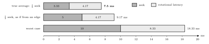
Figure 2: Three access times for the same 7200 rpm disk with a 10 ms edge-to-edge seek, drawn to scale, each a seek (dark) followed by a rotational wait (light). The true average, with both ends of the seek random, is a third of the edge-to-edge seek plus half a turn: 3.33 + 4.17 = 7.5 ms. Taking half the edge-to-edge seek, which is right only if every seek starts at an edge, overstates it at 9.17 ms. The worst case, a seek right across the disk that arrives just after the sector has passed and so waits a whole turn, is 10 + 8.33 = 18.33 ms, more than twice the average. The transfer takes microseconds and is too short to draw.
Virtual I/O: files
A program that wants to save some data should not have to know which drive, head, cylinder and sector it will land on, or what to do when a read times out and has to be retried. The operating system hides all of that behind the file, the abstraction almost all I/O goes through. To the OS a file is just a sequence of bytes; whatever structure it has, lines of text or the header of an image, is the application’s business (file-systems).
File systems
Files are far easier to use, and to program with, when they have names. A file system provides the names: it ties each file, which is really a collection of sectors, to a name in a directory. To do that it sets some sectors aside for its own index information, the File Allocation Table of the FAT file systems being one example, and uses the rest to store the files themselves. There are many file systems, differing in how they organise those tables: FAT, FAT32, exFAT, NTFS, EXT2, EXT3, EXT4, APFS, HFS+, UFS and ZFS among them.
Disk formatting
Formatting happens at two levels. A low-level format rewrites every sector from scratch, its preamble, empty data and ECC, and leaves no file system at all. A high-level format creates an empty file system by writing only the index and table sectors; the data sectors are not touched.
Deleting works the same way as a high-level format, on a smaller scale. The OS removes the file’s index entry and marks its blocks free, but it does not overwrite the sectors that hold the data. The file’s bytes are still there until something new is written over them, which is why deleted files can often be recovered (file-systems).
Files and blocks
Thanks to the OS, a file is called FinalReport.doc rather than by its cylinder and sector numbers. A program writes and reads the file as bytes; the OS keeps a map from the name to the file’s blocks, and from each block to its sectors, with the names arranged in a hierarchy of directories (folders).
Space is handed out in blocks, also called allocation units: one sector, or several consecutive sectors, typically 512 bytes to 32 kB. The block size is a trade-off. Larger blocks mean fewer of them, so a smaller map, but more space wasted at the end of each file (the EOF).
Block size and wasted space
A file fills whole blocks except the last, which is usually only partly used. The rest of that block is wasted. If the amount spilling into the last block is equally likely to be anything up to a full block,
\[\text{wasted space} \approx \frac12\,[\text{block size}]\]
per file, on average. Small blocks cut the file into many pieces with little waste at the end; large blocks cut it into few pieces with a big remainder (file-systems).
Worked: one file, three block sizes
A 10,000-byte file
test.cis stored with 512-byte, 4 kB (4096-byte) or 32 kB (32,768-byte) blocks. How many blocks does it take, and how much space is wasted? With half a block wasted per file on average, how much is wasted over 10,000 files?
The number of blocks is the size divided by the block size, rounded up.
| Block size | Blocks | Space used | Wasted at EOF | Average waste, 10,000 files |
|---|---|---|---|---|
| 512 B | \(\lceil 10000/512 \rceil = 20\) | 10,240 B | 240 B | \(10^4 \times 256 = 2{,}560{,}000\) B |
| 4096 B | \(\lceil 10000/4096 \rceil = 3\) | 12,288 B | 2,288 B | \(10^4 \times 2048 = 20{,}480{,}000\) B |
| 32,768 B | \(\lceil 10000/32768 \rceil = 1\) | 32,768 B | 22,768 B | \(10^4 \times 16384 = 163{,}840{,}000\) B |
In exchange, the map shrinks: a 1 GiB volume has \(2^{30}/512 = 2{,}097{,}152\) blocks to track at 512 B but only \(2^{30}/32768 = 32{,}768\) at 32 kB. The full comparison is in file-systems.
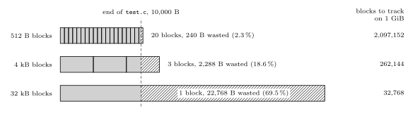
Figure 3: The 10,000-byte file test.c stored with each of the three block sizes, drawn to scale. Grey is the file and hatching the unused end of its last block; each percentage is the share of the space taken that is wasted. With 512-byte blocks the file takes 20 blocks and wastes only 240 bytes, a sliver too thin to see; with 4 kB blocks it takes 3 and wastes 2,288; with one 32 kB block it wastes 22,768 bytes, more than twice the file itself. The column on the right is the other side of the trade: the number of blocks the map must track on a 1 GiB volume falls from over two million to 32,768 as the blocks grow.
Disk allocation
Take a file of 15 sectors, with 1 block = 1 sector, on a surface of five tracks with twelve sectors each.
- (a) Contiguous: blocks 0 to 11 fill one track in order, and 12 to 14 continue on the next track. This is ideal: one seek and one rotational wait reach block 0, blocks 0 to 11 then stream past the head in a single turn, and blocks 12 to 14 cost only a step to the adjacent track and a wait for block 12 to come round.
- (b) Fragmented: the blocks are scattered over every track. That is the likely case, because disks become fragmented as files are created and deleted.
Fragmentation means slow access: each jump to another track costs a seek, and each jump to a sector that is not next under the head costs rotational latency. Both layouts are drawn on one surface in file-systems.
See also
- memory-technologies — classifying memory, SRAM and DRAM, ROM to flash, the ATmega324A’s memories, capacity units
- memory-hierarchy-and-cache — the hierarchy, cache levels, and average access time with a cache
- magnetic-disks — disk geometry, sector format, usable capacity, and the access-time derivations
- file-systems — files, formatting, deleting, block size and allocation
- memory-models · assembly-process — the ATmega324A’s address spaces and the
.cseg,.dsegand.esegsegments - 2026-10-19-floating-point-numbers — Lecture 23