CSSE2010 — Week 5 Notes
Lecture 9 — From Digital Logic to Processors: ALU and Control Unit
The first half of the course, assembled into a processor. See cpu-organisation for the blocks, arithmetic-logic-unit for the ALU and its control table, and fetch-decode-execute-cycle for the control unit’s job. The worked examples, and the thread joining them, are below.
Where this sits
Everything so far has been gates, flip-flops and state machines. They assemble into the three blocks of a CPU: a control unit, an ALU, and registers, joined by internal buses and connected to memory and IO over external buses. Full picture in cpu-organisation.
The control unit fetches instructions from memory and makes the ALU and registers carry them out. There is enough of it below to see why the ALU needs the control inputs it has. The AVR used later in the course is an 8-bit machine with 32 general purpose registers, R0–R31, and therefore an 8-bit ALU.
Registers
Registers are temporary storage inside the CPU, in two kinds:
- General purpose registers — the data being operated on and the results. Collectively the register file; their width is the CPU word size.
- Special purpose registers — used by the system. Two of them: the Program Counter (PC), holding the address of the next instruction to be fetched, and the Instruction Register (IR), holding the current instruction.
Scale varies: a small CPU might have 8 × 8-bit registers, a large one 64 × 32-bit. Drawn out in cpu-organisation.
The ALU
The ALU is versatile hardware which can perform various operations based on some control inputs. A function/control input selects between addition, increment, subtraction, bitwise AND, bitwise OR and so on, so the ALU does considerably more than adding.
Its connections are of two kinds. A, B and Output are data (each an \(n\)-bit bus), while Function/Control is control (\(m\) bits). The ALU is one piece of hardware whose behaviour is chosen by wires coming from somewhere else.
Like adders, ALUs can be made up from 1-bit slices, and an \(n\)-bit ALU is \(n\) identical slices with the carry rippling through. The bit-slice circuit, the cascade and the full table of control combinations are all in arithmetic-logic-unit.
Two levels of control
The slice’s control inputs work at two different levels, and separating them is what makes the whole combinations table make sense:
- Permutations of the data inputs —
ENA,ENB,INVAcondition A and B before any function sees them. - Function select — \(F_1 F_0\) picks which operation’s result reaches the output:
| \(F_1 F_0\) | Function |
|---|---|
| 00 | A and B |
| 01 | invert B |
| 10 | A or B |
| 11 | A plus B |
The first three are logical, the last arithmetic.
What the conditioning gates do
Call the two conditioned lines \(X\) (on the A path) and \(Y\) (on the B path). Three gates produce them, and those three gates are the entire front end of the ALU:
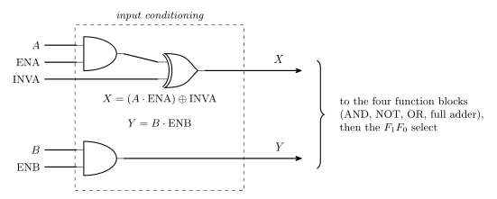
Figure 1: The input-conditioning gates of the bit slice. The two conditioned lines are X on the A path and Y on the B path. Nothing here selects an operation — these gates only decide what the four function blocks downstream get to see, which is why this is a separate level of control.
| ENA | INVA | \(X\) |
|---|---|---|
| 0 | 0 | \(0\) |
| 0 | 1 | \(1\) |
| 1 | 0 | \(A\) |
| 1 | 1 | \(\overline{A}\) |
| ENB | \(Y\) |
|---|---|
| 0 | \(0\) |
| 1 | \(B\) |
Being able to force an operand to a constant 0 or a constant 1 (all ones across the word, which is \(-1\) in two’s complement) is what lets a single ALU produce \(0\), \(1\), \(-1\), \(A+1\), \(B-1\) and \(-A\) with no dedicated hardware for any of them.
The same ALU without a multiplexer
The four-function ALU can be drawn in two forms. The simplified form routes the four results (\(A\) and \(B\), \(\overline{B}\), \(A\) or \(B\), and the adder’s sum) into a multiplexer whose select is \(F_1F_0\) (arithmetic-logic-unit). The full internal diagram, from Tanenbaum’s Structured Computer Organization, has no multiplexer at all: it feeds \(F_1F_0\) into a decoder, and the decoder’s four outputs are enable lines, one per function.
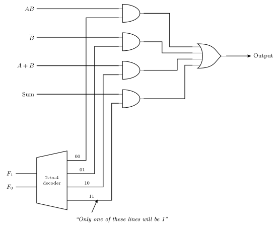
Figure 2: Selecting a function with enable lines instead of a multiplexer: a decoder turns F1 F0 into four enable lines, each function’s result is ANDed with its own enable line, and the four gated results are OR’d together. Because a decoder raises exactly one output, three of the AND gates emit 0 and the OR simply passes the fourth through. The decoder block stands for inverters plus four AND gates. The logical results are labelled AB, B-bar and A+B, but the gates actually see the conditioned X and Y of the previous figure. The enable-to-function mapping is the F1 F0 table above.
Only one of the enable lines is 1 at a time. That is the defining property of a decoder (combinational-logic-blocks), and it is what makes the final OR gate safe: three of its four inputs are guaranteed to be 0, so the OR is not combining anything, just passing the selected result through. The two drawings are therefore the same machine. A multiplexer is a decoder driving enable gates into an OR, which is exactly how the mux of combinational-logic-blocks is built inside.
Two other things the full diagram makes visible that the simplified one hides:
- the three logical functions form a logical unit and the adder is a separate full adder, so the slice is some logic, one adder, and a chooser;
- the carry-in to the adder is Carryin (INC), which is where the
INCcontrol input of the combinations table physically enters.
Example — calculating \(B - A\) using this ALU
The question is which values of \(F_1\), \(F_0\), ENA, ENB, INVA and INC make the ALU output \(B - A\).
Via two’s complement negation:
\[B - A = B + (-A) = B + (\overline{A} + 1) = B + \overline{A} + 1\]
\[\boxed{F_1 = 1 \quad F_0 = 1 \quad \text{ENA} = 1 \quad \text{INVA} = 1 \quad \text{ENB} = 1 \quad \text{INC} = 1}\]
Select the adder (\(F_1F_0 = 11\)), let \(A\) through and invert it (\(\text{ENA} = \text{INVA} = 1\), giving \(X = \overline{A}\)), let \(B\) through (\(\text{ENB} = 1\)), and set the carry into the bottom slice (\(\text{INC} = 1\)). Written as a column addition across the word for \(n = 8\):
\[\begin{array}{cccccc} & B_7 & B_6 & \cdots & B_1 & B_0 \\ + & \overline{A_7} & \overline{A_6} & \cdots & \overline{A_1} & \overline{A_0} \\ + & 0 & 0 & \cdots & 0 & 1 \end{array}\]
The bottom row is INC entering the least significant slice — so the \(+1\) of the negation costs no extra hardware at all.
Useful combinations
The full table of useful combinations of ALU inputs is in arithmetic-logic-unit. Three of its rows, worked through:
- \(B - 1\) — control input by control input: \(F_1F_0 = 11\) (adder), \(\text{ENA} = 0\) with \(\text{INVA} = 1\) so \(X\) is all ones, \(\text{ENB} = 1\) so \(Y = B\), \(\text{INC} = 0\). Across the word that is \(B_7 B_6 \dots B_0\) plus \(1\,1\,\dots\,1\), i.e. \(B + (-1)\).
- \(-1\) — the pattern \(11\dots1\). Here the same all-ones \(X\) is combined by OR with \(Y\) forced to zero, so the all-ones pattern passes straight through to the output.
- \(B + 1\) — by the same reasoning it is \(F_1F_0 = 11\), \(\text{ENA} = 0\), \(\text{ENB} = 1\), \(\text{INVA} = 0\), \(\text{INC} = 1\): force \(X\) to zero, pass \(B\), and add the carry.
The control unit
Fetch-decode-execute
The control unit operates in a continuous cycle on the datapath — fetch an instruction from memory into the CPU (PC and IR are the registers involved), decode it to resolve the opcode and operands, then execute, issuing control signals so the operation happens in the datapath. Written out as five steps, with the PC advancing before execution, and drawn as a loop, in fetch-decode-execute-cycle. The cycle is a three-stage pipeline.
Control signals
The datapath is a register file feeding two buses into the ALU, with the result returning on a destination bus. Controlling it means deciding four things:
- what the ALU does;
- which register values are placed on the A and B buses;
- which register receives the result from the destination bus;
- when to read or write memory.
Each is decided by a bundle of wires leaving the control unit, and their widths follow from the hardware they drive:
| Signal | Width | Why that width |
|---|---|---|
| A register select | 3 | \(2^3 = 8\) registers in the file (r0–r7) |
| B register select | 3 | same |
| Destination select | 3 | same |
| ALU control | 6 | the six ALU control inputs — \(F_1\), \(F_0\), ENA, INVA, ENB, INC |
| Memory read/write | 1 | one bit chooses the direction |
plus address and data lines to memory, and — coming back the other way — the ALU status lines feeding into the control unit. The whole figure is in fetch-decode-execute-cycle.
So r5 = r0 + r2 becomes: A select 0, B select 2, destination select 5, ALU control set to the \(A+B\) row of the combinations table.
Control signals come from the control unit, which must generate them in the right order for a given instruction — and the instruction is determined by the contents of the Instruction Register.
Data influencing control
The IR alone is not enough: the control unit can’t operate without knowing something about the data. If a for-loop variable is meant to run from 10 down to 0, the control unit has to know when it gets there.
That is what the status register is for. It is determined by ALU operations, stores the status of the last ALU operation, and is available to the control unit. if (x < 0) becomes, at this level, an ALU operation followed by the control unit reading a status bit.
ALU status flags
| Flag | Question |
|---|---|
| Z | zero bit — was the last result 0? |
| V | overflow bit — did the last addition/subtraction overflow, assuming a two’s complement operation? |
| C | carry bit — was a carry out generated? |
| N | negative bit — was the result negative as two’s complement, i.e. what is the sign bit? |
Typically held in a special purpose STATUS register (SREG) available to the control unit. The register is wider than four bits, and these four flags occupy its right-hand end.
Example — the flags after \(8_{10} - 9_{10}\) on a 5-bit ALU
First negate 9 in 5 bits: \(9 = 01001\), invert to \(10110\), add one to get \(10111\). Then add, keeping the carries into and out of the sign column:
\[\begin{array}{crl} \text{carry into MSB} \rightarrow & 0\phantom{0000} & \\ & 01000 & \\ + & 10111 & \\ \hline \text{carry out} = 0 \rightarrow & 11111 & \end{array}\]
\[Z = 0 \qquad C = 0 \qquad V = 0 \qquad N = 1\]
- \(Z = 0\) — the result is not zero.
- \(C = 0\) — nothing carried out of the top bit.
- \(V = 0\) — the carry into the sign column and the carry out of it are both 0, so they agree; equivalently, \(8 + (-9) = -1\) is well within 5-bit two’s complement range. See 2026-08-04-binary-arithmetic for the \(C_{in} \oplus C_{out}\) rule.
- \(N = 1\) — the sign bit is set.
And \(11111\) read as two’s complement is \(-1\), which is indeed \(8 - 9\).
See also
- cpu-organisation · arithmetic-logic-unit · fetch-decode-execute-cycle
- binary-number-representations — two’s complement, which the whole subtraction story rests on
- 2026-08-04-binary-arithmetic — the overflow rules the V flag implements
- combinational-logic-blocks — the decoder and multiplexer the function select is built from
- state-machines · logic-gates
- 2026-08-20-state-machines — Lecture 8
Lecture 10 — AVR Introduction
See instruction-set-architecture for machine instructions, the ISA and assembly language, avr-architecture for the chip, and avr-instructions for the instruction set and its encodings.
Outline
- Machine code
- Introduction to AVR — hardware, then assembly language
Recap
Basic computer organisation — ALU, control unit, registers, primary memory (cpu-organisation) — with the fetch-decode-execute cycle running over it: the instruction comes out of primary memory (F), is decoded (D), and is executed against the registers and ALU (E). Everything here is that picture made concrete on a real chip.
Machine code
Machine instructions
An example of Atmel AVR machine code: 0000 1101 0111 0111.
Instructions typically consist of:
- Opcode (operation code) — defines the operation, e.g. addition.
- Operands — what is being operated on, e.g. particular registers or a memory address.
So add rd, rr, meaning rd ← rd + rr, is an opcode (add) plus two register operands. (That example word decodes to a real instruction, worked out below.)
Instruction Set Architecture
An ISA is a specification — i.e. a document. It specifies the interface between hardware and software: software above the line is compiled without knowing how the chip works, hardware below it is built without knowing what will run. Drawn out in instruction-set-architecture.
Microarchitecture
Microarchitecture = the architecture of the control unit — i.e. the state machine (gates and flip-flops etc.) that implements the control unit.
Which is exactly the state-machines material from Lecture 8, now at processor scale.
An ISA can be implemented by many different microarchitectures. The 8086 ISA has been implemented by many processors in different ways; the Pentium ISA by Pentium, Pentium IV, Core2Duo and i7 (each differently), by various AMD devices, and by other manufacturers.
Assembly language
Machine code is too hard to program in, so we use assembly language: human readable (just!), and converted into machine code by software called an assembler.
add r3,r4 |
r3 ← r3 + r4 |
inc r22 |
r22 ← r22 + 1 |
The structural point: a high-level language compiles one-to-many, whereas assembly assembles 1:1 — one assembly instruction is exactly one machine instruction.
Introduction to Atmel AVR
Hardware
Atmel AVR devices are microcontrollers, which include lots of components on one chip: CPU, memory (RAM), program memory, input/output devices. A microprocessor is the CPU alone: an ATmega324A is not a CPU; it contains one, plus everything else needed to make a working system.
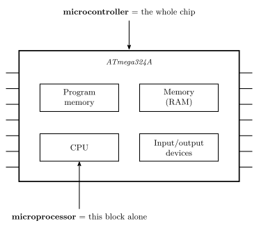
Figure 3: Microcontroller versus microprocessor. The four boxes are the four kinds of component, all in one package. The whole chip is the microcontroller, and only the CPU block is what would be sold on its own as a microprocessor. What a real ATmega324A actually contains is the chip diagram in the AVR architecture note.
On the AVR architecture diagram, the three regions of the cycle fall out of the block layout:
| Blocks | |
|---|---|
| F | Program Counter → Flash Program Memory → Instruction Register |
| D | Instruction Decoder → Control Lines |
| E | 32 × 8 general purpose registers → ALU → Status and Control |
Since those are separate hardware, they run concurrently on successive instructions — a three-stage pipeline. Drawn out, with the sizes and volatility of each memory, in avr-architecture.
Numbers worth having: program memory is 32 kB flash and non-volatile; the register file is 32 registers, R0–R31, each 8 bits wide and made of flip-flops; the ALU is 8-bit, which is what makes AVR an 8-bit machine; data SRAM is 2 kB and volatile; the data bus is 8 bits.
The peripherals on the ATmega324A datasheet block diagram fall into groups: the four 8-bit ports A–D are GPIO; USART 0, USART 1, SPI and TWI are communication; 8-bit T/C 0, 16-bit T/C 1 and 8-bit T/C 2 are the timers/counters; and the A/D converter and analog comparator go together as a fourth group. The 16-bit T/C 3 box is not in the timers/counters group: it belongs to the ATmega1284/1284P rather than the 324A. The three memories are FLASH for the program, SRAM for data, and EEPROM for non-volatile data. Those groupings are drawn out, with the package boundary and internal bus, in avr-architecture.
The AVR status register
8 bits, all R/W, all reset to 0:
| Bit | 7 | 6 | 5 | 4 | 3 | 2 | 1 | 0 |
|---|---|---|---|---|---|---|---|---|
| I | T | H | S | V | N | Z | C |
The five to know are the bottom five — S, V, N, Z, C. Four of them are the flags from Lecture 9 (fetch-decode-execute-cycle); I at bit 7 is the global interrupt enable.
AVR instructions
rd is the destination, rr the source. AVR is a two-operand machine — the destination is also an operand, so add rd, rr computes rd ← rd + rr. A three-operand ISA like ARM writes add rd, r1, r2 instead and leaves both sources alone.
| Instruction | Meaning | Example |
|---|---|---|
MOV rd, rr |
“move”, but actually copy: rd ← rr |
mov r3, r14 |
ADD rd, rr |
add rr to rd |
add r5, r6 → r5 ← r5 + r6 |
AND rd, rr |
bitwise AND into rd |
|
OR rd, rr |
bitwise OR into rd |
|
EOR rd, rr |
bitwise exclusive-OR into rd |
|
LDI rd, number |
load immediate — put the number into rd |
ldi r16, 73 |
LDI works for registers r16 to r31 only, with 8-bit numbers (00000000 to 11111111) — in decimal, the range \(-128\) to \(255\). ldi r0, 5 is not valid: r0 is below r16, so no such instruction exists. The reason is in the encoding, further down.
More instructions in coming weeks.
AVR machine code
Formats and bit-field diagrams in avr-instructions. Three encodings, each with a worked example:
ADD — 0000 11rd dddd rrrr
The 0000 11 is the opcode, bits 15–10; the remaining ten bits are the two five-bit register numbers, each torn into a single top bit and a low nibble. Watch the order in the middle: r (bit 9) comes before d (bit 8), the reverse of how the mnemonic writes them.
add r23, r7. The register numbers in binary, each split across its two fields:
- r23 \(= 16 + 4 + 2 + 1 = \texttt{10111}\), so
d= 1 anddddd=0111 - r7 \(= 4 + 2 + 1 = \texttt{00111}\), so
r= 0 andrrrr=0111
\[\texttt{0000 1101 0111 0111}\]
— which is the example word from the machine instructions section above. Drawn out field by field in avr-instructions.
COM — 1001 010d dddd 0000
Flip all bits (one’s complement). For com r19: r19 \(= 16 + 2 + 1 = \texttt{10011}\), so d = 1 and dddd = 0011:
\[\texttt{1001 0101 0011 0000}\]
LDI — 1110 KKKK dddd KKKK
K is the 8-bit constant, split into two nibbles either side of the register field, and d = register number − 16.
That subtraction is exactly why LDI is restricted to r16–r31: \(2^4 = 16\) — four bits of dddd can only name sixteen registers, and the ISA spends them on the upper half of the file.
Coming up
Instruction Set Architecture — more examples of AVR instructions.
See also
Lab 9 — Microchip Studio and AVR Assembly Introduction
Learning Lab 9, the first assembly lab. See avr-instructions for the instruction set, bit-masking for the masking technique the exercises turn on, and avr-architecture for the status register.
What the lab covers
- AVR assembly language — instruction intro, documentation, machine code equivalent
- Microchip Studio (previously Atmel Studio) — assembling and simulating code
Objectives: you should know how to create a project for the ATmega324A, enter assembly language instructions, build the project, simulate instructions and examine register values.
Documentation
- ATmega324A datasheet — have it open from the start of every remaining lab this semester.
- AVR Instruction Set Manual and AVR Instruction Set Reference
- On Blackboard: Learning resources → Atmel AVR resources
- Follow the Microchip Studio tutorial (
Intro_to_Microchip_Studio.pdf) for the lab tasks — see instruction-set-architecture.
Admin: by the end of semester two USB-A cables are needed for data (one for programming, one for serial communication), one of them from about halfway through. On a personal laptop that may mean a dongle — there are workarounds but they all have downsides, so get one sooner rather than later.
Worked: what is the result of this program?
ldi r16, 0x56
ldi r17, 0x34
add r17, r16
r17 will contain 0x8A, r16 will contain 0x56.
\(\texttt{0x34} + \texttt{0x56} = \texttt{0x8A}\) (that is \(52 + 86 = 138\)), and add rd, rr writes to rd — so r17 takes the sum and r16 is left untouched. An answer that ends with r16 = 0x90 or 0x8A has the destination backwards.
Worked: the status register after a compare
ser r17
ldi r18, 0xF0
cp r17, r18
Z = 0, N = 0, V = 0.
ser r17 sets every bit, so r17 = 0xFF; r18 = 0xF0. Neither ser nor ldi touches a flag, so everything comes from the compare, which computes \(\texttt{0xFF} - \texttt{0xF0} = \texttt{0x0F}\) and throws the result away:
- Z = 0 — the discarded result
0x0Fis not zero. - N = 0 — its MSB is 0.
- V = 0 — as signed values this is \((-1) - (-16) = 15\), comfortably in range.
(C is also 0: no borrow, since \(\texttt{0xFF} \geq \texttt{0xF0}\) unsigned.)
Boolean identities
These identities all hold, and together they are the toolkit the exercises need:
| AND | OR | XOR |
|---|---|---|
| \(X \cdot 0 = 0\) | \(X + 0 = X\) | \(X \oplus 0 = X\) |
| \(X \cdot 1 = X\) | \(X + 1 = 1\) | \(X \oplus X = 0\) |
| \(X \cdot X = X\) | \(X + X = X\) |
Each operation has one value that passes a bit through and one that forces it — which is exactly what makes masking work. \(X \oplus 1 = \overline{X}\) is the identity that makes XOR the toggling operation. Full treatment in bit-masking.
Bit masking
Sometimes only a few bits of a register matter. A bitwise AND can mask out the bits that are not of interest; masking can also selectively set, clear, toggle or extract bits. Status register flags will be set also.
Worked: which r16 values make andi r16, 0x01 set Z?
The even numbers.
0x01 is 0000 0001, so the AND clears every bit except bit 0 and the result is bit 0 alone. Z is set exactly when that result is zero — i.e. when bit 0 of r16 was 0, which is precisely when r16 is even. So a single masked AND is an even/odd test, and more generally any single-bit mask turns Z into a test of that one bit.
NoteProvided task
Exercises
Write an AVR assembly language program which performs the following operations on values 0x55 and \(23_{10}\) and puts the result in the given register:
- Bitwise AND →
r16 - Bitwise OR →
r5 - Bitwise EOR →
r17 - Addition →
r6 - Difference (subtraction) →
r7 - One’s complement (inversion) of
0x55→r8 - Two’s complement (negation) of
0x55→r9
Predict the results and status register values (Z, C, N, V) after each operation. Simulate the code in Microchip Studio and check your predictions.
Write AVR assembly language code snippets to:
- Copy the least significant three bits of register
r7to registerr8. Other bits ofr8should be 0. - Toggle the most significant four bits of register
r9. Other bits should be unchanged. - Clear the least significant four bits of register
r10. Other bits should be unchanged. - Set the most significant four bits of register
r11to be 1. Other bits should be unchanged.
Test these code snippets.
Working — the arithmetic and logic program
The two operands:
\[\texttt{0x55} = \texttt{0101 0101} = 85 \qquad 23_{10} = \texttt{0001 0111} = \texttt{0x17}\]
The constraint that shapes the program: ldi only loads into r16–r31, but five of the seven destinations (r5–r9) are low registers. So the operands are loaded into a pair of high registers and copied down with mov before each operation. mov affects no flags, so each block’s flags come only from its own operation.
The first destination, r16, is also a natural place to hold 0x55 — which would destroy it before the later operations run. Holding the operands in r18/r19 instead avoids that.
    ldi  r18, 0x55       ; first operand
    ldi  r19, 23         ; second operand

    mov  r16, r18        ; --- bitwise AND -> r16
    and  r16, r19

    mov  r5, r18         ; --- bitwise OR -> r5
    or   r5, r19

    mov  r17, r18        ; --- bitwise EOR -> r17
    eor  r17, r19

    mov  r6, r18         ; --- addition -> r6
    add  r6, r19

    mov  r7, r18         ; --- difference -> r7
    sub  r7, r19

    mov  r8, r18         ; --- one's complement of 0x55 -> r8
    com  r8

    mov  r9, r18         ; --- two's complement of 0x55 -> r9
    neg  r9
Predicted results and flags
| Operation | Result | Binary | Z | C | N | V |
|---|---|---|---|---|---|---|
and r16, r19 |
0x15 (21) |
0001 0101 |
0 | unchanged | 0 | 0 |
or r5, r19 |
0x57 (87) |
0101 0111 |
0 | unchanged | 0 | 0 |
eor r17, r19 |
0x42 (66) |
0100 0010 |
0 | unchanged | 0 | 0 |
add r6, r19 |
0x6C (108) |
0110 1100 |
0 | 0 | 0 | 0 |
sub r7, r19 |
0x3E (62) |
0011 1110 |
0 | 0 | 0 | 0 |
com r8 |
0xAA (170) |
1010 1010 |
0 | 1 | 1 | 0 |
neg r9 |
0xAB (171) |
1010 1011 |
0 | 1 | 1 | 0 |
Checking the interesting rows:
add— \(85 + 23 = 108\), no carry out of bit 7, and both operands positive giving a positive result, so V = 0.sub— \(85 - 23 = 62\); \(23 < 85\) so there is no borrow and C = 0.com— \(\overline{\texttt{0101 0101}} = \texttt{1010 1010}\). N = 1 because the MSB is now set, and C = 1 becausecomalways sets the carry flag — not a carry out of anything, just a defined convention.neg— \(\overline{\texttt{0x55}} + 1 = \texttt{0xAA} + 1 = \texttt{0xAB}\), which is \(-85\) read as two’s complement. C = 1 becausenegsets carry unless the result is$00, and V = 0 because V is only set when the result is exactly$80.
The logical operations (and, or, eor) all clear V and leave C completely alone — see avr-instructions. That is why C reads unchanged rather than 0 for the first three rows: it holds whatever it held before the program ran.
Working — the bit manipulation snippets
All four are the same shape: build a mask, pick the instruction that does what you want to the masked bits. The choice follows straight from the identities above, and andi/ori cannot be used because every target here is a low register — so the mask goes into a high scratch register (r16) and the two-register form does the work.
Copy the least significant three bits of r7 to r8, other bits of r8 zero — extract, so AND with 1s on the bits to keep:
    mov  r8, r7
    ldi  r16, 0x07       ; 0000 0111
    and  r8, r16
Toggle the most significant four bits of r9 — toggle, so EOR with 1s on the bits to flip (\(X \oplus 1 = \overline{X}\), \(X \oplus 0 = X\)):
    ldi  r16, 0xF0       ; 1111 0000
    eor  r9, r16
Clear the least significant four bits of r10 — clear, so AND with 0s on the bits to clear (\(X \cdot 0 = 0\), \(X \cdot 1 = X\)):
    ldi  r16, 0xF0       ; 1s mark what to KEEP
    and  r10, r16
Set the most significant four bits of r11 — set, so OR with 1s on the bits to set (\(X + 1 = 1\), \(X + 0 = X\)):
    ldi  r16, 0xF0
    or   r11, r16
The thing worth noticing: 0xF0 is the mask in three of the four, meaning three different things. With and it names the bits that survive; with or and eor it names the bits that change. AND’s mask is written for what you keep, the other two for what you touch — mixing that up is the standard bug.
See also
- bit-masking · avr-instructions · avr-architecture · boolean-algebra
- 2026-08-27-avr-introduction — Lecture 10, the assembly language introduction
- instruction-set-architecture — the Microchip Studio toolchain
Lab 8 — State Machines
Learning Lab 8: two FSM design exercises taken all the way from a state diagram to a Logisim circuit. See state-machines for the notation and the design procedure, and 2026-08-20-state-machines for the lecture.
Method: do the hand design first — state diagram → state table → next state logic and output logic — then implement and test in Logisim. (Also watch the LEC 08 — Example FSM Design 1 & 2 videos on Blackboard.)
Worked: the next Gray code value
0000, 0001, 0011, 0010, …
0110.
Gray code changes exactly one bit between consecutive values. From 0010, the values that differ in one bit are 0011 (already used), 0000 (used), 0110, and 1010. The standard reflected ordering takes 0110 next — after which come 0111, 0101, 0100, 1100, … 1010 is also one bit away, but flipping the most significant bit here breaks the reflection pattern. See binary-number-representations and the encoding table in state-machines.
NoteProvided task
Design Task 1 — Sequence Detector
Draw a state diagram for a system that detects the sequence 001 in a series of bits.
- Input: S
- Output: X
The output X is 1 whenever the sequence 001 is detected on the input S (i.e. 0 followed by 0 followed by 1).
Example input sequence   S = 00101010010001
Example output sequence  X = 00100000010001
Then:
- Write down a 2-dimensional state table
- Choose a state encoding — state encoding = number of flip-flops and their values in each state. Examine different options for state encoding!
- Write down a 1-dimensional state table using your encoding
- Determine Boolean expressions for the output (X) and the next state (flip-flop inputs, D’s) in terms of the current state (flip-flop outputs, Q’s) and input (S)
- Enter the circuit into Logisim and simulate it
Working — Task 1
State diagram
The state has to remember how much of 001 has been matched so far. That gives four states — and the fourth exists only because this is a Moore machine, so “I have just detected it” must be a state of its own in order to have an output of its own.
| State | Means | X |
|---|---|---|
| \(S_0\) | no useful progress (last bit was a 1, or just started) | 0 |
| \(S_1\) | seen 0 |
0 |
| \(S_2\) | seen 00 |
0 |
| \(S_3\) | just detected 001 |
1 |
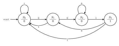
Figure 4: The 001 detector. Every state has two arrows out, one per value of S, which is completeness for a one-input machine. The self-loop on S2 is the important one: a run of three or more zeros stays ready to detect, rather than falling back. From S3 the last bit consumed was a 1, so it behaves exactly like S0 — same transitions, different output.
NoteDiagram conventions
Each state is a circle divided by a chord, with the name above and the output below. A transition is a plain single-headed arrow, labelled with a bare 0 or 1 for a one-input machine. Two more conventions in the figure above:
- The start state is marked by an incoming reset arrow from nowhere.
- A self-loop is an arrow from a state back to itself. The completeness rule (transition arrows from each state must encompass all possibilities, exactly once) guarantees most machines need them.
See csse2010-diagram-notation for the full list of conventions.
Traced against the example sequence in the task, this machine reproduces the example output exactly; the trace is worked out edge by edge below.
2-dimensional state table
| Current state | Next state (\(\overline{S}\)) | Next state (\(S\)) | X |
|---|---|---|---|
| \(S_0\) | \(S_1\) | \(S_0\) | 0 |
| \(S_1\) | \(S_2\) | \(S_0\) | 0 |
| \(S_2\) | \(S_2\) | \(S_3\) | 0 |
| \(S_3\) | \(S_1\) | \(S_0\) | 1 |
Choosing an encoding
Four states, so two flip-flops. The choice genuinely matters, which is what the instruction to examine different options is getting at.
The obvious assignment \(S_0 = 00\), \(S_1 = 01\), \(S_2 = 10\), \(S_3 = 11\) gives three product terms for \(D_1\) and three more for \(D_0\) — nothing collapses.
Now look at the 2-D table again: the \(\overline{S}\) column and the \(S\) column each contain only two distinct destinations, and on \(S = 1\) every state goes to either \(S_0\) or \(S_3\). If the encoding is arranged so that one flip-flop bit tracks the input directly, that bit’s logic disappears entirely. Assigning
\[S_0 = 01 \qquad S_1 = 00 \qquad S_2 = 10 \qquad S_3 = 11\]
does exactly that.
1-dimensional state table
| State | \(Q_1 Q_0\) | \(S\) | Next state | \(D_1 D_0\) | X |
|---|---|---|---|---|---|
| \(S_0\) | 01 | 0 | \(S_1\) = 00 | 0 0 | 0 |
| \(S_0\) | 01 | 1 | \(S_0\) = 01 | 0 1 | 0 |
| \(S_1\) | 00 | 0 | \(S_2\) = 10 | 1 0 | 0 |
| \(S_1\) | 00 | 1 | \(S_0\) = 01 | 0 1 | 0 |
| \(S_2\) | 10 | 0 | \(S_2\) = 10 | 1 0 | 0 |
| \(S_2\) | 10 | 1 | \(S_3\) = 11 | 1 1 | 0 |
| \(S_3\) | 11 | 0 | \(S_1\) = 00 | 0 0 | 1 |
| \(S_3\) | 11 | 1 | \(S_0\) = 01 | 0 1 | 1 |
Boolean expressions
Reading the \(D_0\) column: it is 1 in exactly the four rows where \(S = 1\), and 0 in the four where \(S = 0\).
\[\boxed{D_0 = S}\]
A direct wire from the input to the flip-flop — no gate at all. Reading \(D_1\), which is 1 at \((Q_1Q_0, S) = (00,0), (10,0), (10,1)\):
\[D_1 = \overline{Q_1}\,\overline{Q_0}\,\overline{S} + Q_1\overline{Q_0}\,\overline{S} + Q_1\overline{Q_0}S = \overline{Q_0}\left[\overline{S}(\overline{Q_1} + Q_1) + Q_1 S\right] = \overline{Q_0}\left[\overline{S} + Q_1 S\right]\]
and by the redundancy (simplification) theorem, \(\overline{S} + Q_1 S = \overline{S} + Q_1\):
\[\boxed{D_1 = \overline{Q_0}\,(Q_1 + \overline{S})}\]
\(X\) is 1 only in \(S_3 = 11\):
\[\boxed{X = Q_1 \cdot Q_0}\]
Checking it, edge by edge
Running the expressions against the sequence the task supplies, one column per clock edge — the state shown is the one the machine is in after that edge, and X is that state’s output:
S       =    0  0  1  0  1  0  1  0  0  1  0  0  0  1
state       S1 S2 S3 S1 S0 S1 S0 S1 S2 S3 S1 S2 S2 S3
Q1 Q0       00 10 11 00 01 00 01 00 10 11 00 10 10 11
X       =    0  0  1  0  0  0  0  0  0  1  0  0  0  1
which is X = 00100000010001, the example output sequence in the task, exactly. The three detections land on the final 1 of each 001, including the one at the very end, and the 000 at positions 11–13 shows the self-loop on \(S_2\) doing its job: a third zero keeps the machine ready instead of dropping it back to the start.
The circuit
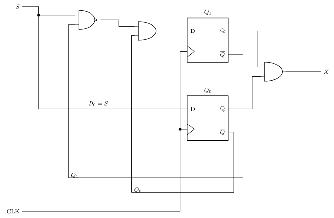
Figure 5: The 001 detector as a logic diagram, the circuit the task’s last bullet asks for (enter the circuit into Logisim and simulate it). Three things the algebra hides are visible here. D0 is a bare wire from the input S to a flip-flop, with no gate anywhere in the path. Both complements the next-state logic needs come off the flip-flops’ own Qbar pins, so the circuit contains no inverter. And the output AND sits to the right of the flip-flops, fed by Q1 and Q0 only - never by S - which is exactly what makes this a Moore machine. The two long return wires at the bottom carry Qbar1 and Qbar0 back to the gates; lines that cross without a junction dot are not connected.
Challenge — the detector in three chips
The challenge is to implement the sequence detector with just three chips: three 74-series packages, total, for Figure 5.
Two D flip-flops are one 74HCT74, leaving two chips for the logic. The trick is that \(\overline{Q_0}\) and \(\overline{Q_1}\) come free from the flip-flops’ complementary outputs, so no inverter package is needed — and De Morgan turns the OR into a NAND that can use \(\overline{Q_1}\) directly:
\[Q_1 + \overline{S} = \overline{\overline{Q_1} \cdot S} \quad\Longrightarrow\quad D_1 = \overline{Q_0} \cdot \operatorname{NAND}(\overline{Q_1},\, S)\]
| Signal | Built from |
|---|---|
| \(D_0 = S\) | a wire |
| \(D_1\) | one NAND + one AND, using \(\overline{Q_0}\) and \(\overline{Q_1}\) from the flip-flops |
| \(X = Q_1 Q_0\) | one AND |
| Chip | Used for |
|---|---|
74HCT74 dual D flip-flop |
\(Q_1\), \(Q_0\) |
74HCT00 quad NAND |
1 gate |
74HCT08 quad AND |
2 gates |
Three chips, with three of the four NAND gates and two of the four AND gates spare. See device-pinouts for the pinouts and circuit-schematics for the drawing rules.
NoteProvided task
Design Task 2 — Sequence Matching
Consider a sequence matching system with
- 2 inputs A, B
- 2 outputs X, Y
- X is 1 if A and B have been the same value (i.e. both 0 or both 1) twice or more in a row, otherwise 0
- Y is 1 if the A and B values are different, otherwise 0
- Initially the A and B values are assumed to have been different and Y should be 1
Draw a state diagram and discuss with tutoring staff. Implement: write down a 2-D state table, choose a state encoding, write down a 1-D state table, determine Boolean expressions for the outputs and the next state (flip-flop inputs, D’s) in terms of the current state (flip-flop outputs, Q’s) and inputs, and enter the circuit into Logisim and simulate.
Working — Task 2
Reducing the inputs
A and B never matter individually — only whether they agree. Define
\[M = \overline{A \oplus B} \qquad (M = 1 \text{ when } A = B)\]
so the four input combinations collapse to two cases, and 00 behaves identically to 11.
State diagram
The machine must remember how long the current run of matches is, capped at two:
| State | Means | X | Y |
|---|---|---|---|
| \(D\) | the last pair differed — the reset state | 0 | 1 |
| \(M_1\) | matched once (the pair before differed) | 0 | 0 |
| \(M_2\) | matched twice or more in a row | 1 | 0 |
That the reset state is \(D\) with \(Y = 1\) is given by the specification: initially the A and B values are assumed to have been different and Y should be 1.
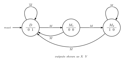
Figure 6: The sequence matcher, with M meaning A equals B. Any mismatch drops straight back to D from anywhere, so the run counter resets in one clock; a match walks D to M1 to M2, where it stays. The two outputs are each true in exactly one state, which is what makes the encoding below collapse the output logic to nothing.
2-dimensional state table
| Current state | \(AB = 00\) (\(M\)) | \(01\) (\(\overline{M}\)) | \(10\) (\(\overline{M}\)) | \(11\) (\(M\)) | X | Y |
|---|---|---|---|---|---|---|
| \(D\) | \(M_1\) | \(D\) | \(D\) | \(M_1\) | 0 | 1 |
| \(M_1\) | \(M_2\) | \(D\) | \(D\) | \(M_2\) | 0 | 0 |
| \(M_2\) | \(M_2\) | \(D\) | \(D\) | \(M_2\) | 1 | 0 |
Choosing an encoding
Three states, so two flip-flops, with one code left over. Each output is true in exactly one state, so if the two flip-flops are made to be the two outputs, the output logic vanishes entirely. Take \(Q_1 = X\) and \(Q_0 = Y\):
\[D = 01 \qquad M_1 = 00 \qquad M_2 = 10 \qquad (11 \text{ unused})\]
\[\boxed{X = Q_1} \qquad \boxed{Y = Q_0}\]
1-dimensional state table
| State | \(Q_1 Q_0\) | \(M\) | Next state | \(D_1 D_0\) | X | Y |
|---|---|---|---|---|---|---|
| \(D\) | 01 | 0 | \(D\) = 01 | 0 1 | 0 | 1 |
| \(D\) | 01 | 1 | \(M_1\) = 00 | 0 0 | 0 | 1 |
| \(M_1\) | 00 | 0 | \(D\) = 01 | 0 1 | 0 | 0 |
| \(M_1\) | 00 | 1 | \(M_2\) = 10 | 1 0 | 0 | 0 |
| \(M_2\) | 10 | 0 | \(D\) = 01 | 0 1 | 1 | 0 |
| \(M_2\) | 10 | 1 | \(M_2\) = 10 | 1 0 | 1 | 0 |
Boolean expressions
\(D_0\) is 1 in exactly the rows where \(M = 0\):
\[\boxed{D_0 = \overline{M} = A \oplus B}\]
\(D_1\) is 1 at \((Q_1Q_0, M) = (00, 1)\) and \((10, 1)\), so \(Q_1\) is a don’t-care:
\[D_1 = \overline{Q_1}\,\overline{Q_0}M + Q_1\overline{Q_0}M = \overline{Q_0}M(\overline{Q_1} + Q_1) \quad\Longrightarrow\quad \boxed{D_1 = \overline{Q_0} \cdot M}\]
Writing \(E = A \oplus B\) so that \(M = \overline{E}\), De Morgan folds \(D_1\) into a single gate:
\[D_1 = \overline{Q_0} \cdot \overline{E} = \overline{Q_0 + E} = \operatorname{NOR}(Q_0,\, A \oplus B)\]
So the whole circuit is one XOR feeding both a flip-flop input and a NOR, with the outputs taken straight off the flip-flops.
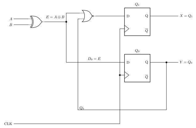
Figure 7: The sequence matcher as a logic diagram. One XOR does all of the input reduction: E = A xor B is simultaneously D0 and one input of the NOR that forms D1. Because the encoding was chosen so that the two flip-flops are the two outputs, X and Y are taken straight off Q1 and Q0 and there is no output logic at all - the entire machine is two gates and two flip-flops. The one feedback wire, Q0 back to the NOR, is the whole of the next-state logic that depends on the state. Lines crossing without a junction dot are not connected.
At chip level that NOR is the awkward part. The course’s parts list has quad NAND, AND, OR and XOR packages plus a hex inverter, but no NOR — see device-pinouts. Rewriting \(D_1 = \overline{Q_0}\cdot\overline{E}\) as an AND of two complements fixes it: \(\overline{Q_0}\) is free from the flip-flop and \(\overline{E}\) is one inverter on the XOR output, giving 74HCT86 + 74HCT04 + 74HCT08 + 74HCT74, four chips.
Checking the unused state
The encoding leaves \(Q_1Q_0 = 11\) unassigned, so it is worth confirming the machine cannot get stuck there (the same lock-up check as week4-lab-lab-7-exercises). Substituting \(Q_1Q_0 = 11\):
\[D_1 = \overline{Q_0}\cdot M = 0 \cdot M = 0 \qquad D_0 = \overline{M}\]
so from 11 the machine goes to 01 (\(D\)) when \(M = 0\), or 00 (\(M_1\)) when \(M = 1\). Both are legal states, so it self-corrects within one clock — no lock-up, and no extra logic needed to guarantee it.
See also
- state-machines · sequential-circuits · flip-flops-and-latches · [counters]
- 2026-08-20-state-machines — Lecture 8
- circuit-schematics · device-pinouts — for the three-chip challenge
- binary-number-representations — Gray code
- csse2010-diagram-notation — the state-diagram and logic-diagram conventions these figures follow
Reference material
Arithmetic Logic Unit
The ALU is versatile hardware which can perform various operations based on some control inputs — it does considerably more than adding. See cpu-organisation for where it sits in the CPU, and combinational-logic-blocks and logic-gates for the pieces it is built from.
The ALU as a block
A function/control input indicates the operation the ALU is to perform: addition, increment (\(+1\)), subtraction, bitwise AND, bitwise OR, and so on.
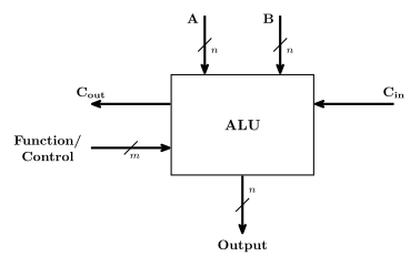
Figure 8: The ALU as a block. A and B are n-bit data inputs and Output is the n-bit result; the m-bit Function/Control input selects which operation is performed, and the carry in and out let several ALUs be chained. Slashes mark bus widths.
Like adders, ALUs can be made up from 1-bit slices — an \(n\)-bit ALU is \(n\) identical circuits, one per bit position.
The 1-bit ALU (bit slice)
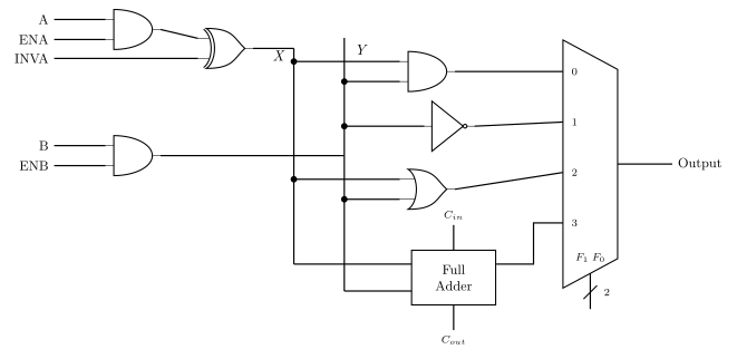
Figure 9: One bit slice. The ENA/INVA/ENB gates on the left condition the two data inputs into internal signals X and Y; the four function blocks in the middle compute AND, NOT, OR and sum from them simultaneously; the multiplexer selects which one reaches the output, under the F1 F0 select. Cin and Cout belong to the full adder, and are what chain one slice to the next.
\(F_1\) and \(F_0\) select which of the four function blocks reaches the output:
| \(F_1 F_0\) | Function | |
|---|---|---|
| 00 | A and B | logical |
| 01 | invert B | logical |
| 10 | A or B | logical |
| 11 | A plus B | arithmetic |
Two levels of control
The bit slice has control inputs at two distinct levels, and keeping them apart is what makes the combinations table below readable:
- Permutations of the data inputs —
ENA,ENBandINVAcondition A and B before any function sees them. - Function select — \(F_1 F_0\) picks which operation’s result is actually output.
The conditioning gates are worth working out explicitly, because most of the useful ALU tricks come from them rather than from the function select. Writing \(X\) for the conditioned A line and \(Y\) for the conditioned B line:
\[X = (A \cdot \text{ENA}) \oplus \text{INVA} \qquad\qquad Y = B \cdot \text{ENB}\]
| ENA | INVA | \(X\) | ENB | \(Y\) | |
|---|---|---|---|---|---|
| 0 | 0 | 0 | 0 | 0 | |
| 0 | 1 | 1 | 1 | \(B\) | |
| 1 | 0 | \(A\) | |||
| 1 | 1 | \(\overline{A}\) |
So the A line can be forced to a constant 0, a constant 1 (all ones across the whole word, i.e. \(-1\) in two’s complement), \(A\) itself, or \(\overline{A}\) — and that constant-generating ability is what lets one ALU compute \(-1\), \(B-1\) and \(B - A\) without any dedicated hardware for them.
INC is the third conditioning input: it is the carry into the least significant slice, 0 for addition and 1 for increment.
Cascading into an \(n\)-bit ALU
A machine word is \(n\) bits (often 8, 16, 32, …), and an \(n\)-bit ALU is built from \(n\) identical bit slices.
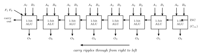
Figure 10: An 8-bit ALU as eight cascaded slices. Each slice takes its own bit of A and B and produces its own bit of the output; the carry out of one slice is the carry in of the next, rippling from right (least significant) to left. F1, F0, ENA, ENB and INVA are shared by every slice, so all eight always perform the same operation.
\(F_1\), \(F_0\), ENA, ENB and INVA are shared between all bit slices — there is one function select for the whole ALU, not one per bit. Only the carry is per-slice, and it ripples through from right to left, which is exactly the ripple-carry adder behaviour from earlier in the course.
Useful combinations of ALU inputs
Everything a single ALU can be made to do, by choosing the six control inputs. This table is worth understanding rather than memorising — each row follows from \(X\), \(Y\) and the function select above.
| \(F_1\) | \(F_0\) | ENA | ENB | INVA | INC | Function |
|---|---|---|---|---|---|---|
| 1 | 0 | 1 | 0 | 0 | 0 | \(A\) |
| 1 | 0 | 0 | 1 | 0 | 0 | \(B\) |
| 1 | 0 | 1 | 0 | 1 | 0 | \(\overline{A}\) |
| 0 | 1 | 1 | 1 | 0 | 0 | \(\overline{B}\) |
| 1 | 1 | 1 | 1 | 0 | 0 | \(A + B\) |
| 1 | 1 | 1 | 1 | 0 | 1 | \(A + B + 1\) |
| 1 | 1 | 1 | 0 | 0 | 1 | \(A + 1\) |
| 1 | 1 | 0 | 1 | 0 | 1 | \(B + 1\) |
| 1 | 1 | 1 | 1 | 1 | 1 | \(B - A\) |
| 1 | 1 | 0 | 1 | 1 | 0 | \(B - 1\) |
| 1 | 1 | 1 | 0 | 1 | 1 | \(-A\) |
| 0 | 0 | 1 | 1 | 0 | 0 | \(A\) AND \(B\) |
| 1 | 0 | 1 | 1 | 0 | 0 | \(A\) OR \(B\) |
| 1 | 0 | 0 | 0 | 0 | 0 | \(0\) |
| 1 | 1 | 0 | 0 | 0 | 1 | \(1\) |
| 1 | 0 | 0 | 0 | 1 | 0 | \(-1\) |
Reading a few rows to see the pattern:
- \(A\) — select OR (\(F_1F_0 = 10\)), pass \(A\) through (\(X = A\)), force the other side to zero (\(Y = 0\) via \(\text{ENB} = 0\)). \(A + 0 = A\) in the OR sense.
- \(-1\) — select OR, force \(X\) to all ones (\(\text{ENA}=0\), \(\text{INVA}=1\)) and \(Y\) to zero. All ones is \(-1\) in two’s complement.
- \(B - 1\) — select the adder, \(Y = B\), $X = $ all ones \(= -1\), and no extra carry. So \(B + (-1)\).
- \(1\) — select the adder with both inputs forced to zero and \(\text{INC} = 1\), so the result is the carry alone.
Worked example — computing \(B - A\)
What are the values of \(F_1\), \(F_0\), ENA, ENB, INVA and INC to calculate \(B - A\)?
The route is two’s complement negation:
\[B - A = B + (-A) = B + (\overline{A} + 1) = B + \overline{A} + 1\]
So the ALU needs \(\overline{A}\) on one adder input, \(B\) on the other, and a carry of 1 into the bottom slice:
| Control | Value | Why |
|---|---|---|
| \(F_1 F_0\) | 1, 1 | select the adder |
| ENA | 1 | let \(A\) through |
| INVA | 1 | invert it, giving \(\overline{A}\) |
| ENB | 1 | let \(B\) through |
| INC | 1 | the \(+1\) of the negation |
Laid out as a column addition across the word, this is:
\[\begin{array}{cccccc} & B_7 & B_6 & \cdots & B_1 & B_0 \\ + & \overline{A_7} & \overline{A_6} & \cdots & \overline{A_1} & \overline{A_0} \\ + & 0 & 0 & \cdots & 0 & 1 \end{array}\]
The final row is the INC carry entering at the least significant slice and rippling left — which is why the \(+1\) costs no extra hardware at all.
Overflow: the flag the carry-out does not give you
Every arithmetic row of the table above can go wrong in the same way: the true answer needs more bits than the word has. The ALU still produces a result, and it is a wrong one — so something has to say so.
The carry-out is not that something. \(C_{out}\) in Figure 8 is the correct overflow test for unsigned arithmetic and the wrong one for two’s complement. In two’s complement a carry out of the top slice is routine and is simply discarded (1111 + 1111 gives a carry out and the perfectly correct answer \(-2\)), while \(0111 + 0001\) produces no carry out at all and is nonetheless an overflow. The signed test is whether the top slice’s carry in and carry out disagree:
\[V = C_{n} \oplus C_{n-1}\]
and equivalently, in terms of signs: overflow happens exactly when the two operands share a sign and the result does not. Adding two positives cannot legitimately give a negative; adding two negatives cannot legitimately give a positive.
When \(C_{n-1}\) is not available
That formula assumes you can reach the carry into the most significant slice, which inside your own cascade of bit slices you can. On a single-package adder you cannot: a 74HCT283 wires \(C_1\), \(C_2\) and \(C_3\) stage-to-stage inside the chip and brings out only \(C_0\) and \(C_4\) (see device-pinouts). Learning Lab 3 makes exactly this its extension task — build an overflow LED using only \(A_3\), \(B_3\), \(S_3\) and \(C_4\) — so the sign form is the one you actually wire:
\[V = A_3 B_3 \overline{S_3} + \overline{A_3}\,\overline{B_3} S_3\]
Read literally: (both operands negative and the sum positive) or (both operands positive and the sum negative). With only the two-input gates the course’s parts list stocks, the same function factors into three gates — “the signs agree” AND “the sum disagrees with them”:
\[V = (A_3 \odot B_3) \cdot (A_3 \oplus S_3)\]
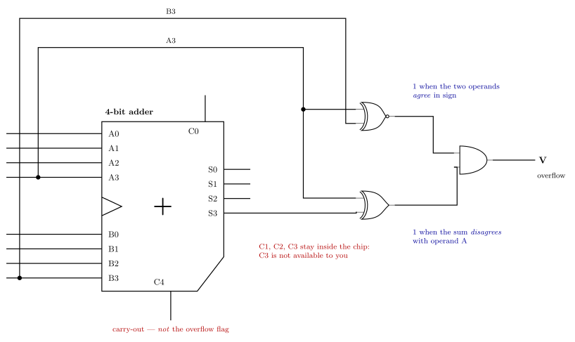
Figure 11: Two’s complement overflow detected from the pins a packaged adder actually brings out. A3 and B3 are tapped from the operand inputs and S3 from the sum output; the XNOR asks whether the two operands agree in sign and the XOR asks whether the sum disagrees with them, and overflow is both at once. C4 is deliberately left going nowhere, because the carry-out is the unsigned overflow test, not this one. The adder outline, the ‘+’ glyph and the input/output placement follow the course’s 74HCT283 schematic symbol.
There is a cheaper form still. A full adder gives \(S_3 = A_3 \oplus B_3 \oplus C_3\), so the missing internal carry can be recovered as \(C_3 = A_3 \oplus B_3 \oplus S_3\), and substituting into \(V = C_4 \oplus C_3\) leaves
\[V = C_4 \oplus A_3 \oplus B_3 \oplus S_3\]
— three two-input XOR gates, all four of which fit in a single 74HCT86.
Back to \(B - A\)
The worked example above computes \(B - A\) as \(B + \overline{A} + 1\), and it is an ordinary addition as far as the top slice is concerned — so it is the conditioned operand that the overflow test must look at. The sign bit entering the adder is \(\overline{A_{n-1}}\), not \(A_{n-1}\), which is why a subtraction of two numbers whose signs differ is the case that can overflow, while an addition of two numbers whose signs differ never can. See week2-lab-binary-arithmetic for the lab build and 2026-08-04-binary-arithmetic for the arithmetic behind the rule.
See also
- cpu-organisation · fetch-decode-execute-cycle
- binary-number-representations — two’s complement, which every subtraction row above relies on
- combinational-logic-blocks — the multiplexer and decoder used inside the slice
- 2026-08-24-alu-and-control-unit — Lecture 9
AVR Architecture
The Atmel AVR: what is on the chip, how the CPU is laid out, and where the fetch-decode-execute cycle happens in it. See cpu-organisation for the generic picture this specialises and avr-instructions for what it executes.
Microcontroller, not microprocessor
Atmel AVR devices are microcontrollers. A microcontroller includes lots of components on one chip:
- CPU
- Memory (RAM)
- Program memory
- Input/output devices
That is the distinction from a microprocessor, which is the CPU alone. An ATmega324A is not a CPU — it contains a CPU, alongside memory and a large collection of peripherals, so that a useful system can be one chip rather than a board full of them.
The AVR CPU
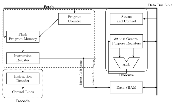
Figure 12: The AVR CPU core, with the three stages of the cycle marked. Fetch (dashed) reads the next instruction from flash under the program counter into the instruction register; decode (dotted) turns it into control lines; execute (solid) runs it over the register file, ALU and status register, with the 8-bit data bus tying everything together. The two lines dropping to the Data SRAM are the direct and indirect addressing routes — both come out of the instruction, which is why they leave from the instruction register. The execute group takes in the status register, the register file and the ALU; the Data SRAM sits outside it.
Reading the diagram as the cycle of fetch-decode-execute-cycle:
| Stage | Blocks involved |
|---|---|
| Fetch | Program Counter → Flash Program Memory → Instruction Register |
| Decode | Instruction Register → Instruction Decoder → Control Lines |
| Execute | General purpose registers → ALU → back to registers, with Status and Control updated |
Because these three groups are largely separate hardware, the AVR overlaps them: while one instruction executes, the next is being fetched. This course calls it a three-stage pipeline. The ATmega164A/324A/644A/1284P datasheet describes the core as “single level pipelining”, i.e. fetch and execute overlapping, which is two stages. Answer three-stage pipeline in the exam, but the datasheet is the authority on the hardware.
The pieces
| Block | Notes |
|---|---|
| Flash program memory | Holds the program. 32 kB on the ATmega324A, and non-volatile — it survives power loss |
| Program Counter | Addresses flash to select the next instruction — the PC of cpu-organisation |
| Instruction Register | Holds the instruction currently being worked on |
| Instruction Decoder | Turns the instruction’s bits into control lines — this is the control unit |
| 32 × 8 general purpose registers | R0–R31, each 8 bits wide, built from flip-flops |
| ALU | 8-bit, so AVR is an 8-bit machine |
| Status and Control | Holds the flags the ALU produces — N, Z, C, V among others |
| Data SRAM | 2 kB, volatile — static RAM, i.e. flip-flops |
| Data bus | 8 bits wide, tying the execute-side blocks together |
Two addressing routes reach the SRAM, drawn as the two vertical paths in Figure 12 — direct addressing (the address is in the instruction) and indirect addressing (the address is in a register). Both leave from the instruction register, because in either case it is the instruction that says which cell is wanted; they differ only in whether it says so with a literal address or with the name of a pointer. Both, and the other two modes, are in addressing-modes.
Four numbers define the chip: the flash is 32 kB and non-volatile; the SRAM is 2 kB, volatile, and made of static flip-flops; the register file is 32 registers, r0…r31, each 8 bits wide and made of flip-flops; and the ALU is 8-bit, which makes the AVR an 8-bit machine.
The register file
General purpose registers (0–31) are quite regular and can be used interchangeably. Two exceptions are worth having by heart:
- A few instructions work on half the registers (r16–r31), because only 4 bits are used to represent the operand in the instruction and \(2^4 = 16\).
LDI,SER,ANDI,ORIandCPIare among them — see avr-instructions. - X, Y and Z are register pairs that double as 16-bit pointers.
X, Y and Z
The top six registers of the file are those three pairs, low byte in the lower-numbered register:
| Pointer | High : Low | Register addresses |
|---|---|---|
| X | R27 : R26 | 0x1B : 0x1A |
| Y | R29 : R28 | 0x1D : 0x1C |
| Z | R31 : R30 | 0x1F : 0x1E |
Two 8-bit registers side by side make a 16-bit address — which is what the data space needs and no single 8-bit register can hold. They are what indirect addressing uses: ld r5, X means “load from wherever X points”, and the instruction only has to name which pointer, so it stays one word (addressing-modes).
The low byte living in the lower-numbered register is the same little-endian convention the AVR uses in memory (memory-models).
Address spaces
The AVR is a Harvard machine — separate address spaces for instructions and data — so 0x0000 names two entirely different locations depending on which space is meant, and the instruction decides.
Data address space — 0x0000 to 0x08FF
| Region | Addresses | Size |
|---|---|---|
| 32 Registers | 0x0000–0x001F |
32 |
| 64 I/O Registers | 0x0020–0x005F |
64 |
| 160 Ext I/O Reg. | 0x0060–0x00FF |
160 |
| Internal SRAM | 0x0100–0x08FF |
2048 bytes (2 kB) |
The register file and all 224 I/O registers are mapped into the data space, ahead of the SRAM. That is what lets lds/sts reach an I/O register by its data address while in/out reach the first 64 by their I/O register number — the two numbering systems differ by exactly the 0x20 the register file occupies. Details in avr-io-ports.
The datasheet draws the SRAM box as 1024/2048/4096/16384 × 8 because the diagram covers the whole ATmega164A/324A/644A/1284P family; the 324A is the 2048 entry, which is what puts the top of the data space at 0x08FF.
Program memory — 0x0000 to 0x3FFF
\(2^{14}\) 16-bit words: 16,384 instruction words = 32,768 bytes = 32 kB. The datasheet splits it into an Application Flash Section and, at the highest addresses, a Boot Flash Section.
0x3FFF \(= 2^{14} - 1\), and the sizing arithmetic — why 32 kB of program memory is 14 address bits rather than 15 — is worked through in memory-models. The short version: the cells are 16 bits wide, so there are half as many of them as there are bytes.
The AVR status register
8 bits, all readable and writable, all reset to 0:
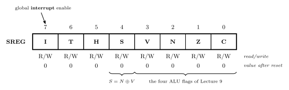
Figure 13: The status register, in the three-row form the datasheet uses: bit numbers above, flag names in the boxes, then the access row and the value each bit takes after reset. The callout names bit 7, the global interrupt enable; the braces underneath mark the four ALU flags and the sign flag \(S = N \oplus V\).
Instruction descriptions refer to these as SREG(n) by bit number:
| Flag | Bit | Meaning |
|---|---|---|
| C | SREG(0) | carry — was a carry out generated? |
| Z | SREG(1) | zero — was the result 0? |
| N | SREG(2) | negative — the sign bit of the result |
| V | SREG(3) | overflow — did a two’s complement addition/subtraction overflow? |
| S | SREG(4) | sign, \(= N \oplus V\) — the sign of the result corrected for any overflow |
| H | SREG(5) | half-carry — carry out of bit 3 |
| T | SREG(6) | transfer bit, used by BLD and BST |
| I | SREG(7) | global interrupt enable — set by sei, cleared by cli; cleared by the hardware when it takes an interrupt and set again by reti (avr-interrupts) |
C, Z, N and V are exactly the four flags of fetch-decode-execute-cycle.
S is not simply “the sign bit” — that is N. \(S = N \oplus V\) means: the result is negative (with no overflow), or would have been negative had overflow not occurred. That correction is what makes signed comparisons work, which is why the signed branches (BRLT, BRGE) test S while the unsigned ones (BRLO, BRSH) test C. The four cases — including the overflow case where N alone gives the wrong answer — are drawn in 2026-09-14-flow-of-control, and the branch pairs are tabulated in avr-branches-and-jumps.
The one-line meanings and the SREG(n) numbering are those of Atmel’s AVR Instruction Set Manual and the instruction summary in the ATmega324A datasheet. The I/O register map is the I/O register summary, pages 636–639 of the ATmega164A/324A/644A/1284P datasheet, which writes the I/O register number first and the data memory address in parentheses after it.
On-chip peripherals (ATmega324A)
Beyond the CPU and its memories, the chip carries a large set of peripherals — this is what makes it a microcontroller rather than a processor. The two figures nest: the whole of Figure 12 is what sits inside the single box marked AVR CPU in Figure 14.
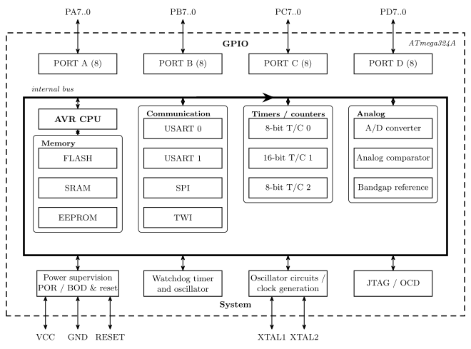
Figure 14: What is on the ATmega324A: the datasheet block diagram, rearranged into clusters by kind of thing — GPIO, memory, communication, timers/counters, analog and system. The dashed outline is the package boundary and the heavy rectangle inside it the internal bus, both as the datasheet draws them; the individual peripheral-to-port wiring is left out.
| Group | On the chip |
|---|---|
| General purpose I/O | PORT A, PORT B, PORT C, PORT D — four 8-bit ports |
| Communication | USART 0, USART 1, SPI, TWI |
| Timers/counters | 8-bit T/C 0, 16-bit T/C 1, 8-bit T/C 2 (T/C 3 is on the ATmega1284/1284P, not the 324A — the family datasheet’s block diagram covers both) |
| Analog | A/D converter, analog comparator, internal bandgap reference |
| Memory | Flash (program), SRAM (data), EEPROM (data, non-volatile) |
| System | Power supervision (POR/BOD & reset), watchdog timer and oscillator, oscillator/clock generation (XTAL1, XTAL2), JTAG/OCD |
There are three memories with three different jobs: flash for the program, SRAM for volatile working data, and EEPROM for data that must survive a power cycle. SRAM and EEPROM are the pair to keep straight: both hold data, and they differ only in surviving a power cycle.
See also
- cpu-organisation · fetch-decode-execute-cycle · instruction-set-architecture
- avr-instructions — the instruction set this hardware runs
- avr-io-ports — the I/O registers and the four GPIO ports
- avr-interrupts — the I bit, the vector table and the peripherals’ interrupt sources
- avr-timers-and-counters · avr-usart · avr-spi · analog-to-digital-conversion — four of the peripherals in detail
- memory-models · addressing-modes — the two address spaces, and how instructions name them
- assembly-process — flash, SRAM and EEPROM as the assembler’s three segments
- memory-technologies — flash, SRAM and EEPROM as technologies, and what the boot loader section is for · memory-hierarchy-and-cache — where the registers and SRAM sit by speed, and why the AVR needs no cache
- binary-number-representations — the flags’ two’s complement interpretation
- 2026-08-27-avr-introduction — Lecture 10
- 2026-08-31-instruction-set-architecture-part-1 — Lecture 11
AVR Instructions
The AVR instructions introduced so far, in assembly and in machine code. See instruction-set-architecture for what an instruction set is and avr-architecture for the hardware that runs these.
The full alphabetical instruction set — each mnemonic with its operation, description, flags affected, clock count, opcode pattern and an example — is in the AVR instruction set reference: Atmel’s AVR Instruction Set Manual, and the instruction summary in the ATmega324A datasheet the course says to keep open. The notation key immediately below and the per-instruction flag table at the end are unverified against that reference — check them against your own copy before leaning on them.
Reading the instruction set reference
Operand notation — how an operand’s allowed values map onto opcode bits:
| Notation | Meaning | Values | Opcode pattern |
|---|---|---|---|
Rd |
destination register (may be a source too) | r0…r31 | ddddd |
| r16…r31 | dddd (register number − 16) |
||
Rr |
source register | r0…r31 | rrrrr |
Rh:Rl |
register pair as a 16-bit quantity | r25:r24 / X / Y / Z | dd (00 / 01 / 10 / 11) |
K |
constant data | 0…255 | KKKKKKKK |
k |
constant address | −64…63, −2048…2047, 0…65535 | kkkkkkk … kkkk kkkk kkkk kkkk |
b |
bit number in a register | 0…7 | bbb |
s |
bit in the status register | 0…7 | sss |
P |
I/O register number | 0…63 | PPPPPP |
q |
displacement for direct addressing | 0…63 | qqqqqq |
The Rd row is the whole story behind LDI’s restriction — an instruction spending five bits on the register gets all 32; one spending four gets sixteen, and pays for it by starting at r16.
Operation notation — used in the Operation column:
M[a] / PM[a] / IO[a] |
SRAM cell / program memory (flash) byte / I/O register at address a |
PC / SP / STACK |
program counter / stack pointer / M[SP] |
← |
assigned value |
reg(a) |
bit a of register reg, numbered 7…0 most to least significant |
Flag names in the Flags Affected column are the SREG bits of avr-architecture.
Register conventions
Two operand names recur throughout the instruction set:
rd— the destination register.rr— the source register.
AVR is a two-operand machine: the destination is also one of the sources, so add rd, rr means rd ← rd + rr. (Contrast a three-operand ISA such as ARM, where add rd, r1, r2 leaves both sources untouched.) This matters when reading code — an AVR arithmetic instruction always overwrites one of its inputs.
Instructions by type
The instruction set can be cut two ways.
By what the instruction touches — the instruction-type list of instruction-set-architecture, filled in with the instructions so far:
| Type | Does | AVR so far |
|---|---|---|
| Input/Output | communicate with I/O devices/ports | IN, OUT |
| Load/Store | move data from/to memory | LD, LDS, ST, STS |
| Move | copy data between registers | MOV |
| Arithmetic | addition, subtraction, … | ADD, ADC, SUB, INC, NEG |
| Logical | Boolean operations | AND, ANDI, OR, ORI, EOR, COM |
| Branching | deciding which instruction to perform next | JMP, BREQ, BRNE |
By operand count, which splits the arithmetic and logical group instead:
| AVR examples | ||
|---|---|---|
| Dyadic | combine 2 operands to produce a result | add r5, r6 (arithmetic) · and r5, r6 (logical, bitwise) |
| Monadic | one operand → one result | ser r16 (set) · clr r5 (clear) · neg r5 (2’s complement) · com r5 (1’s complement) · the shifts and rotates |
The second cut is the one that predicts the syntax: a dyadic instruction has a comma in it, a monadic one does not.
The instructions so far
| Instruction | Meaning | Example |
|---|---|---|
MOV rd, rr |
copy contents of rr into rd — rd ← rr |
mov r3, r14 |
ADD rd, rr |
add contents of rr to rd — rd ← rd + rr |
add r5, r6 |
ADC rd, rr |
add with carry — rd ← rd + rr + C |
adc r11, r5 |
AND rd, rr |
bitwise AND, result into rd |
|
OR rd, rr |
bitwise OR, result into rd |
|
EOR rd, rr |
bitwise exclusive-OR, result into rd |
|
INC rd |
rd ← rd + 1 |
inc r22 |
LDI rd, number |
load immediate — put the number into rd |
ldi r16, 73 |
SER rd |
set all bits — rd ← $FF. Same as ldi rd, 0xFF, so r16–r31 only |
ser r17 |
CLR rd |
clear all bits — rd ← 0. Same as eor rd, rd, so any register |
clr r3 |
SUB rd, rr |
rd ← rd − rr |
sub r7, r19 |
COM rd |
one’s complement — flip all bits | com r8 |
NEG rd |
two’s complement — negate | neg r9 |
ANDI rd, K |
bitwise AND with a constant — r16–r31 only | andi r16, 0x01 |
ORI rd, K |
bitwise OR with a constant — r16–r31 only | ori r16, 0xF0 |
MOV is named misleadingly: it copies, it does not move. The source register is unchanged. It also affects no flags, which is what makes it safe to shuffle values between operations without disturbing the status register.
SER and CLR are short-hand ways of setting/clearing all bits of a register, and their restrictions differ because their expansions do:
| Exactly the same as | Reaches | |
|---|---|---|
ser rd (set register) |
ldi rd, 0xFF |
r16–r31 only — it inherits LDI’s four-bit register field |
clr rd (clear register) |
eor rd, rd |
any register, r0–r31 — EOR is a two-register instruction with five bits for each |
So clr r3 is legal and ser r3 is not, which looks arbitrary until you look at what each one assembles to. clr is also the reason \(X \oplus X = 0\) from bit-masking is worth remembering: XORing a register with itself is how the machine zeroes one.
Compare instructions
These do the arithmetic, discard the result, and keep only the flags — which is exactly what a conditional branch needs.
| Instruction | Does | Note |
|---|---|---|
CP rd, rr |
rd − rr |
compares two registers |
CPI rd, K |
rd − K |
compares against a constant — like ldi, r16–r31 only |
TST rd |
rd AND rd |
examines one register; literally the same operation as and rd, rd |
tst looks odd until you notice that ANDing a value with itself leaves it unchanged (\(X \cdot X = X\)) but still sets N and Z from it — so it is a zero/sign test that costs nothing and clobbers nothing. See bit-masking.
A comparison is the same as subtraction, with the result not saved — it exists only to set status register flags (Z, N, C, V …). And the instruction reference specifies which status register bits are set by which instructions: the flags are defined per instruction rather than falling out of one shared adder, which is the point of the table at the end of this note.
Branch instructions
Based on status register values — the flags a compare just set:
Branches to label if |
|
|---|---|
BREQ label |
Z = 1 |
BRNE label |
Z = 0 |
Together with CP that is a complete conditional: compare, which sets Z exactly when the two operands were equal, then branch on Z.
    cp   r5, r6          ; r5 - r6, result thrown away, flags kept
    breq same            ; Z = 1, i.e. r5 == r6
JMP label is the unconditional version — it tests nothing and always goes. Labels, and the program skeleton the branches live in, are in avr-program-structure.
breq/brne are two of ten: there is one branch per status flag per value, and the pairs that matter for ordering are brsh/brlo (unsigned, on C) and brge/brlt (signed, on S) — the full table, and why the signed pair reads S rather than N, are in avr-branches-and-jumps.
Control flow
The instructions that write the PC, and the two stack instructions that go with the calls (avr-branches-and-jumps, procedures-and-the-stack):
| Instruction | Does | Words | Cycles |
|---|---|---|---|
BRxx label |
branch if a flag has the wanted value; reach ±64 words | 1 | 1 (not taken) / 2 (taken) |
JMP label |
PC ← address of label |
2 | 3 |
RJMP label |
PC ← PC + offset; reach ±2 K words | 1 | 2 |
IJMP |
PC ← Z | 1 | 2 |
CALL label |
push the return address, then as JMP |
2 | 4 |
RCALL label |
push the return address, then as RJMP |
1 | 3 |
ICALL |
push the return address, then as IJMP |
1 | 3 |
RET |
pop the return address into PC | 1 | 4 |
PUSH rr |
store rr at SP, SP ← SP − 1 |
1 | 2 |
POP rd |
SP ← SP + 1, load rd from SP |
1 | 2 |
None of these touches the status register except by what the pushed and popped values happen to be; a call between a cp and its branch is safe only if the procedure preserves the flags, which in practice means it is not.
Three more belong to interrupts, and between them they are the only instructions that change the I bit (avr-interrupts):
| Instruction | Does | Words | Cycles |
|---|---|---|---|
SEI |
I ← 1: interrupts enabled | 1 | 1 |
CLI |
I ← 0: interrupts disabled | 1 | 1 |
RETI |
pop the return address into PC, and I ← 1 | 1 | 4 |
RETI is RET plus set I. A handler that ends in RET returns to the right place and leaves interrupts off for good.
Data movement
Data is usually copied, not moved — in every instruction below the source is left alone. What changes is where the two ends are:
| Direction | Called | AVR |
|---|---|---|
| register → register | move | mov |
| memory → register | load | lds, ld |
| register → memory | store | sts, st |
| I/O register → register | input | in |
| register → I/O register | output | out |
Three different places a value can live — a general purpose register, data memory, an I/O register — and a different instruction family for each. The one thing that is genuinely out of reach is SRAM from in/out: P only goes up to 0x3F, so those two never leave the first 64 I/O registers.
Everything else is a question of cost and numbering, not reachability. Because the I/O registers are mapped into the data space (avr-io-ports), lds/sts can reach one — in r16, 0x09 and lds r16, 0x29 both read PIND, the second for two instruction words instead of one. The bug to actually watch for is writing the I/O register number where the data address belongs, or the reverse.
Load and store
| Does | Addressing | Words | Cycles | |
|---|---|---|---|---|
LD rd, X |
rd ← Mem[X] |
indirect — address in the pointer register | 1 | 2 |
ST X, rr |
Mem[X] ← rr |
indirect | 1 | 2 |
LDS rd, k |
rd ← Mem[k] |
direct — 16-bit address in the instruction | 2 (32 bits) | 2 |
STS k, rr |
Mem[k] ← rr |
direct | 2 | 2 |
For example:
    ld   r5, X           ; r5 <- Mem[X]
    st   X, r5           ; Mem[X] <- r5
    lds  r5, 0x20        ; r5 <- Mem[0x20]
    sts  0x20, r5        ; Mem[0x20] <- r5
Both pairs reach the same data space — the difference is only where the address comes from (addressing-modes), and lds/sts pay a second instruction word for spelling it out. X here is the pointer pair of avr-architecture.
In and out
| Does | Words | Cycles | |
|---|---|---|---|
IN rd, P |
rd ← I/O register P |
1 | 1 |
OUT P, rr |
I/O register P ← rr |
1 | 1 |
rd/rr may be any of r0–r31 — unlike ldi, these are not restricted to the top half — and P is an I/O register number 0–63 (0x00–0x3F) or a name from m324Adef.inc. Examples: in r5, 0x26 (I/O register 0x26 is TCNT0) and out PORTD, r6. Full treatment in avr-io-ports.
One word and one cycle makes these the cheapest access on the chip — cheaper than reaching the very same register through lds/sts, which is the whole reason the first 64 I/O registers are special.
Shifts and rotates
Monadic instructions that move every bit one place. They differ only in what arrives at the vacated end and what happens to the bit that falls off — and in all five, the bit that falls off lands in C.
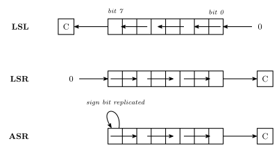
Figure 15: The three shift instructions. LSL and LSR feed a 0 into the vacated end; ASR feeds the sign bit back into itself, which is what makes it a signed division. In all three the bit shifted out lands in the carry flag.
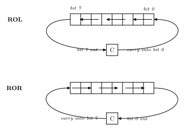
Figure 16: The two rotate instructions. A rotate is a shift whose vacated end is fed from the carry flag instead of a constant, so the register and C together behave as a nine-bit ring.
| Name | Into the vacated end | Out | |
|---|---|---|---|
LSL rd |
Logical Shift Left | 0 → bit 0 |
bit 7 → C |
LSR rd |
Logical Shift Right | 0 → bit 7 |
bit 0 → C |
ASR rd |
Arithmetic Shift Right | bit 7 replicated into itself | bit 0 → C |
ROL rd |
ROtate Left through carry | C → bit 0 | bit 7 → C |
ROR rd |
ROtate Right through carry | C → bit 7 | bit 0 → C |
What they compute
Shifting a binary number one place is multiplying or dividing it by two, which is the whole reason these exist. Using four bits for legibility:
| Worked example | ||
|---|---|---|
LSL |
× 2 | 0010 (2) → 0100 (4) → 1000 (8) |
LSR |
÷ 2, read unsigned | 0110 (6) → 0011 (3); 1000 (8 unsigned) → 0100 (4) |
ASR |
÷ 2, read signed | 1000 (\(-8\)) → 1100 (\(-4\)) |
LSR and ASR are the pair to keep straight. Given 1000, LSR produces 0100 — right if the value meant unsigned 8, wrong if it meant \(-8\). ASR replicates the sign bit into the vacated position and produces 1100 \(= -4\). The same bits go in; the instruction is where you declare which interpretation you meant (binary-number-representations).
There is no matching pair going the other way, because left shifts need no such distinction: a 0 always enters at the bottom, and the signed and unsigned readings of “× 2” agree — right up until the result stops fitting in eight bits.
Shifting a value wider than eight bits
Rotates exist to carry a bit from one byte into the next. To multiply the 16-bit unsigned value in r13:r14 by two (so r13 is the high byte, r14 the low):
    lsl  r14             ; low byte x2; bit 7 falls out into C
    rol  r13             ; high byte x2, pulling C into its bit 0
LSL on the low byte pushes its top bit into C; ROL on the high byte pulls exactly that bit back in at the bottom. The two instructions together shift a sixteen-bit quantity one place.
The wrong answers are worth naming, because each fails differently. lsl r13 (and asl r13, which is the same operation under another name — shifting left, a 0 always enters) shifts the high byte but feeds it a 0, discarding the bit the low byte just produced. rol r14 rotates the wrong byte.
Building wider operations from 8-bit ones
The AVR supports exactly one data type in hardware — an 8-bit integer (instruction-set-architecture). Everything wider is a sequence of instructions, and C is what stitches the pieces together.
Add the 16-bit quantity r5:r4 to r11:r10, result in r11:r10 — high byte named first, so r4 and r10 are the low bytes:
    add  r10, r4         ; r10 <- r10 + r4        (low bytes; carry out lands in C)
    adc  r11, r5         ; r11 <- r11 + r5 + C    (high bytes, plus that carry)
ADD on the low bytes leaves any carry out of bit 7 in C, and ADC on the high bytes adds it back in — the same column-by-column carrying as long addition on paper, one byte per column.
The order is not negotiable, and neither is what sits between the two lines: adc has to run after the add that produced the carry, and any instruction in between that touches C ruins the result. That is the general shape of multi-byte arithmetic on an 8-bit machine — low end first, and nothing allowed to disturb the flag in the middle.
Constants
Constants do not have to be hexadecimal. All five of these load the same value into r17:
| Written | Radix | |
|---|---|---|
ldi r17, 0x34 |
hexadecimal | 0x prefix |
ldi r17, $34 |
hexadecimal | $ prefix |
ldi r17, 52 |
decimal | no prefix |
ldi r17, 064 |
octal | a leading 0 |
ldi r17, 0b00110100 |
binary | 0b prefix |
\(\texttt{0x34} = 52 = 64_8 = \texttt{0b00110100}\). The octal form is the trap: a leading zero changes the radix, so 012 is 10, not 12.
LDI’s restrictions
LDI is the one with strings attached:
- Registers r16 to r31 only. Not r0–r15.
- 8-bit numbers,
00000000to11111111. Written in decimal the range is \(-128\) to \(255\) — that span covers both the signed and the unsigned reading of eight bits.
A counter-example, and the legal version of it:
    ldi  r0, 5           ; NOT legal - r0 is below r16
    ldi  r16, 5          ; the same idea, in a register ldi can reach
The register restriction is not arbitrary: it falls straight out of the encoding below, which has only four bits for the register number.
Machine code
Each instruction is a 16-bit word made of an opcode and operand bit fields — see instruction-set-architecture. In the AVR datasheet’s notation, a format like 0000 11rd dddd rrrr means the literal bits are fixed and each letter is one bit of an operand, gathered from wherever it appears.
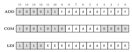
Figure 17: Three AVR instruction encodings, each 16 bits. Fixed opcode bits are shaded; letters are operand bits. In ADD and LDI the operand bits are not contiguous — the register number’s top bit sits apart from the rest, and LDI’s constant is split into two nibbles either side of the register field.
ADD — 0000 11rd dddd rrrr
The opcode is bits 15–10, 0000 11 — six fixed bits, all that is left once the two five-bit register numbers have taken ten of the sixteen. The destination register number is d dddd — five bits, so all 32 registers — and the source is r rrrr. Both have their top bit separated from the other four, and note the order in the middle nibble: the source’s top bit (r, bit 9) comes before the destination’s (d, bit 8), even though the mnemonic writes the destination first.
Worked example: add r23, r7.
| Register | In binary (5 bits) | Split as | |
|---|---|---|---|
rd |
r23 = 16 + 4 + 2 + 1 | 10111 |
d = 1, dddd = 0111 |
rr |
r7 = 4 + 2 + 1 | 00111 |
r = 0, rrrr = 0111 |
Dropping those into 0000 11rd dddd rrrr:
\[\texttt{0000 1101 0111 0111}\]
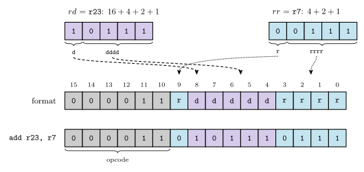
Figure 18: Assembling add r23, r7. Each register number is written as five bits, then torn in two: the top bit goes into the middle nibble and the low four into their own field. Shading, not position, is what tells the two operands apart here. The two guide lines cross because the destination’s bit sits between the source’s two pieces.
COM — 1001 010d dddd 0000
Flip all bits — one’s complement. One register operand, again as d dddd.
Worked example: com r19. r19 = 16 + 2 + 1 = 10011, so d = 1 and dddd = 0011:
\[\texttt{1001 0101 0011 0000}\]
LDI — 1110 KKKK dddd KKKK
Two operand fields:
K— the 8-bit constant, split into two nibbles: the high four bits in the firstKKKKfield, the low four in the last.d— the register number minus 16.
That subtraction is why LDI only reaches r16–r31: the field is four bits, so it can express \(2^4 = 16\) distinct registers, and the ISA spends them on the top half of the register file.
Applying the rule to ldi r16, 73: \(d = 16 - 16 = 0\), so dddd = 0000; \(73 = \texttt{0100 1001}\), so the high nibble is 0100 and the low nibble 1001:
\[\texttt{1110 0100 0000 1001}\]
Flags, by instruction
The reference’s Flags Affected column is worth reading rather than assuming — the flags are defined per instruction, not derived from a single adder. For the instructions above:
| Instruction | Z | C | N | V |
|---|---|---|---|---|
MOV, LDI, SER |
— | — | — | — |
AND, ANDI, OR, ORI, EOR, TST |
from result | unchanged | from result | cleared to 0 |
ADD, ADC, SUB, CP, CPI |
from result | from carry/borrow | from result | signed overflow |
CLR |
always 1 | unchanged | always 0 | cleared to 0 |
COM |
from result | always set to 1 | from result | cleared to 0 |
NEG |
from result | set unless the result is $00 |
from result | set only if the result is $80 |
Two of these will catch you out. The logical operations leave C alone entirely — whatever it held before an and it still holds after. And COM sets C unconditionally, which is not a carry out of anything; it is a defined convention, chosen so that com followed by an increment behaves like a negation.
The CLR row is just the logical row with a result that is guaranteed to be 0x00 — clr rd is eor rd, rd — which makes it the one instruction whose flags you can predict without knowing the operand.
For the shift, rotate and branch instructions, look the flags up in the reference rather than guessing. The one part that is visible in the diagrams above is C: every shift and rotate sets it from the bit that fell out. The rest is defined per instruction, as the paragraph opening this section warns.
For ADD specifically, the manual gives the flags as Boolean formulas over the operand and result bits, writing \(R\) for the result (which equals Rd after the operation):
\[N = R_7 \qquad Z = \overline{R_7}\cdot\overline{R_6}\cdot\overline{R_5}\cdot\overline{R_4}\cdot\overline{R_3}\cdot\overline{R_2}\cdot\overline{R_1}\cdot\overline{R_0}\] \[V = Rd_7 \cdot Rr_7 \cdot \overline{R_7} + \overline{Rd_7}\cdot\overline{Rr_7}\cdot R_7 \qquad C = Rd_7 \cdot Rr_7 + Rr_7 \cdot \overline{R_7} + \overline{R_7}\cdot Rd_7\]
\(Z\) is a NOR over every result bit. \(V\) says overflow happened exactly when both operands had the same sign and the result’s differs — two negatives giving a positive, or two positives giving a negative. And \(S = N \oplus V\), for signed tests. See avr-architecture.
See also
- instruction-set-architecture · avr-architecture · bit-masking
- avr-io-ports — the I/O registers
in/outreach - addressing-modes — the four ways an operand names its value
- avr-program-structure — labels,
jmpand the program skeleton - avr-interrupts —
sei,cli,reti, and which flags an interrupt handler must save - binary-number-representations — one’s and two’s complement, and the \(-128\) to \(255\) range
- 2026-08-27-avr-introduction — Lecture 10
- 2026-09-03-instruction-set-architecture-part-2 — Lecture 12
Binary Number Representations
Bits, bytes, and words
- Bit = binary digit (0 or 1).
- Nibble = 4 bits. It is the unit that makes hexadecimal convenient (one hex digit = one nibble).
- Byte = 8 bits, e.g.
01010111. - Modern computers deal with words, usually a power-of-2 number of bytes: 1, 2, 4, or 8 bytes = 8, 16, 32, 64 bits. The AVR used in this course is at the small end — an 8-bit (1-byte) word; modern CPUs sit at the other end, 32- or 64-bit.
Representing whole (unsigned) numbers
Each bit position has a value — a power of 2, increasing from right (least significant) to left (most significant). Binary → decimal: add the values of each position where the bit is 1.
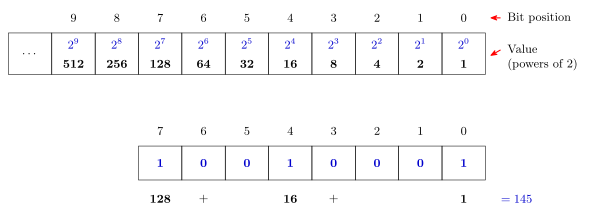
Figure 19: Place values for an unsigned binary number, and a worked conversion. Position \(i\) is worth \(2^i\), so reading a binary number is just adding the place values of the positions holding a 1: \(10010001_2 = 128 + 16 + 1 = 145\).
Most and least significant bits
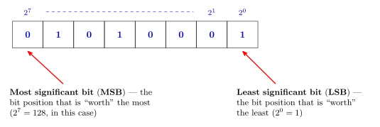
Figure 20: The two ends of a word get names, because almost every later convention (shifting, sign bits, bit numbering in AVR registers) is stated in terms of them. For an \(n\)-bit unsigned word the MSB is worth \(2^{n-1}\) — here \(2^7 = 128\) — and the LSB is always worth \(2^0 = 1\).
Converting decimal to binary
Two equivalent methods, both worked on the same number, 53.
Method 1 — sum of powers of 2. Rewrite \(n\) as a sum of powers of 2, by repeatedly subtracting the largest power of 2 not greater than \(n\) (\(53 - 32 = 21\), \(21 - 16 = 5\), \(5 - 4 = 1\), \(1 - 1 = 0\)). Then assemble the binary number from 1’s in the bit positions corresponding to those powers of 2, and 0’s everywhere else.
Figure 21: Method 1 on \(53\). Each power of two in the decomposition names one bit position — \(2^5\) is position 5, \(2^4\) is position 4, and so on — and every position with no term in the sum gets a 0. Reading the row off left to right gives \(00110101_2\).
Method 2 — repeated division. Build the bits up from the right (least significant): divide \(n\) by 2, the remainder (0 or 1) is the next bit, then repeat with \(n\) = the quotient. Stop when the quotient reaches 0, and read the remainders upwards.
Figure 22: Method 2 on \(53\). The remainders come out LSB-first, which is why the answer has to be read back up the column: \(110101_2\), or \(00110101_2\) padded to a byte. The same procedure with a divisor of 16 or 8 converts to hexadecimal or octal instead.
Number range (unsigned)
- Smallest representable value: all 0’s → 0.
- Largest representable value: all 1’s → for an \(n\)-bit word, \(2^n - 1\) (e.g. 255 for 8 bits).
The \(-1\) is the part worth understanding: an \(n\)-bit word has \(2^n\) distinct patterns, but one of them is spent on zero.
Figure 23: Why the largest unsigned value is \(2^n-1\) and not \(2^n\). Counting up from all-zeros steps through every pattern in turn — each extra bit doubles how many there are, so 8 bits give \(2^8 = 256\) patterns — and because the count starts at 0, the last one is 255.
Other radices
Radix = number system base. A radix-\(k\) number system has \(k\) distinct symbols for digits \(0\) to \(k-1\), and the value of each digit (from the right) is \(k^0, k^1, k^2, \dots\) — so a radix-\(k\) number \(d_{m}\dots d_1 d_0\) is worth \(\sum_i d_i k^i\). E.g. \(1\mathrm{A}_{16} = 1 \cdot 16^1 + 10 \cdot 16^0 = 16 + 10 = 26\).
- Octal (radix-8): symbols
0–7. One octal digit corresponds to exactly 3 bits. - Hexadecimal (radix-16): symbols
0–9,A–F. One hex digit corresponds to exactly 4 bits — very convenient for grouping binary.
| Dec | 0 | 1 | 2 | 3 | 4 | 5 | 6 | 7 | 8 | 9 | 10 | 11 | 12 | 13 | 14 | 15 | 16 | 17 |
|---|---|---|---|---|---|---|---|---|---|---|---|---|---|---|---|---|---|---|
| Oct | 0 | 1 | 2 | 3 | 4 | 5 | 6 | 7 | 10 | 11 | 12 | 13 | 14 | 15 | 16 | 17 | 20 | 21 |
| Hex | 0 | 1 | 2 | 3 | 4 | 5 | 6 | 7 | 8 | 9 | A | B | C | D | E | F | 10 | 11 |
Converting binary ↔︎ hex/octal by grouping
Because \(16 = 2^4\) and \(8 = 2^3\), no arithmetic is needed: group the bits from the right — four at a time for hex, three at a time for octal — and translate each group with the table above. Pad the leftmost group with leading zeros.
Figure 24: One bit pattern read two ways. Grouping \(00011010_2\) into nibbles from the right gives \(1\) and \(\mathrm{A}\), i.e. \(1\mathrm{A}_{16}\); grouping the same bits in threes gives \(0\), \(3\) and \(2\), i.e. \(32_{8}\). The grouping must start at the right — starting at the left gives the wrong answer whenever the width is not a multiple of 3 or 4.
The same trick read backwards is why hex is used for bit patterns at all: a full byte of 1’s, 1111 1111, is F F = \(\mathtt{0xFF}\) = 255, and any byte can be written as two hex digits.
To convert decimal → any radix, use Method 2 with that radix as the divisor: \(26 \div 16\) gives quotient 1 remainder 10 (= A), so \(26_{10} = 1\mathrm{A}_{16}\); \(26 \div 8\) gives quotient 3 remainder 2, so \(26_{10} = 32_8\). See 2026-07-27-course-intro-bits-bytes-binary for that worked exercise.
Radix notation conventions
Since a bare number like 101 or 747 is ambiguous, a radix indicator is needed. A subscript works generically (e.g. \(101_2\), \(101_{16}\)); in code/assembly, conventions vary. Bolded rows are the ones this course mostly uses:
| Radix | Convention | Example | Where used |
|---|---|---|---|
| any | subscript | \(101_2\), \(101_{16}\) | generic/mathematical |
| Hex | leading 0x |
0x101 |
C, Atmel AVR |
| Hex | trailing h |
101h |
some assembly languages |
| Hex | leading $ |
$747 |
Atmel AVR assembly |
| Octal | leading 0 |
0101 |
C, Atmel AVR |
| Octal | trailing q |
101q |
some assembly languages |
| Octal | leading @ |
@747 |
some assembly languages |
| Binary | leading 0b |
0b101 |
Atmel AVR assembly, some C |
| Binary | trailing b |
101b |
some assembly languages |
| Binary | leading % |
%101 |
some assembly languages |
The octal convention is the trap: in C, a leading 0 silently changes the radix, so 0101 is \(65_{10}\), not \(101_{10}\).
Representing signed numbers
Computers don’t store \(+\) and \(-\) signs; the sign has to be encoded in the bits themselves. Four formats have been used, and all four — plus unsigned — represent positive numbers identically. Only the negatives differ.
Signed magnitude
The leftmost bit is a sign bit (0 positive, 1 negative) and contributes nothing to the magnitude. Negate by inverting the sign bit alone.
Ones’ complement
The sign bit now also carries weight: its position value is \(-(2^{N-1}-1)\). Negate by inverting all the bits.
Two’s complement
The sign bit’s position value is \(-2^{N-1}\). Negate by inverting all the bits and adding 1. This is the one actually used in practice.
Compare the position values, 8-bit:
| bit 7 | 6 | 5 | 4 | 3 | 2 | 1 | 0 | |
|---|---|---|---|---|---|---|---|---|
| Signed magnitude | sign | 64 | 32 | 16 | 8 | 4 | 2 | 1 |
| Ones’ complement | \(-127\) | 64 | 32 | 16 | 8 | 4 | 2 | 1 |
| Two’s complement | \(-128\) | 64 | 32 | 16 | 8 | 4 | 2 | 1 |
Excess-\(2^{N-1}\)
For 8 bits, “excess 128”: the value stored is the true value plus 128. So \(-3\) is stored as \(125\) and \(3\) as \(131\).
It is exactly two’s complement with the sign bit reversed — a 0 in the MSB means bit value \(-128\), a 1 means 0. Its practical use is that comparing two signed numbers becomes simple in hardware. The exponent of an IEEE floating-point number is stored in excess notation for exactly that reason, with a bias one smaller: excess-127 for 8 bits (floating-point-numbers).
Ranges
| Format | 8-bit | \(n\)-bit |
|---|---|---|
| Unsigned | \(0\) to \(255\) | \(0\) to \(2^n - 1\) |
| Signed magnitude | \(-127\) to \(127\) | \(-(2^{n-1}-1)\) to \(2^{n-1}-1\) |
| Ones’ complement | \(-127\) to \(127\) | \(-(2^{n-1}-1)\) to \(2^{n-1}-1\) |
| Two’s complement | \(-128\) to \(127\) | \(-2^{n-1}\) to \(2^{n-1}-1\) |
| Excess-\(2^{n-1}\) | \(-128\) to \(127\) | \(-2^{n-1}\) to \(2^{n-1}-1\) |
Worked example — \(\pm 47\) in 8 bits
\(+47 = \texttt{00101111}\) in every format.
| Format | \(-47\) | How |
|---|---|---|
| Signed magnitude | 10101111 |
flip the sign bit |
| Ones’ complement | 11010000 |
invert all bits |
| Two’s complement | 11010001 |
invert all bits, add 1 |
| Excess-128 | 01010001 |
\(-47 + 128 = 81\) |
And in 4 bits, \(-3\) is 1100 in ones’ complement and 1101 in two’s complement.
Why “complement”?
A thing and its complement together make a whole — an angle and its complement make a right angle, a set and its complement a universal set.
- Ones’ complement: a number plus its negative gives a string of ones (
11111111in 8 bits). - Two’s complement: a number plus its negative gives a power of two, with overflow (
1 00000000). It would more accurately be called power-of-two’s complement.
Base 10 has the same pair — nines’ and ten’s complement — used on early mechanical adding machines to do subtraction.
Why two’s complement wins
Two representations of zero, which wastes a bit pattern that could have extended the range:
- Signed magnitude:
00000000and10000000 - Ones’ complement:
00000000and11111111
Asymmetric range: two’s complement and excess-\(2^{n-1}\) (one more negative than positive).
Arithmetic: signed-magnitude addition requires taking cases; ones’ complement addition requires an extra addition step (the end-around carry); sign extension and comparison are non-trivial in both. Two’s complement has a single zero and its addition is just binary addition — no special cases.
Format matters
The same eight bits mean different things under different formats. 10010010 reads as:
| Read as | Value |
|---|---|
| Unsigned | 146 |
| Two’s complement | \(-110\) |
| Ones’ complement | \(-109\) |
| Signed magnitude | \(-18\) |
| Excess-128 | 18 |
Or 01010101: 85 unsigned, \(-43\) in excess-128, 'U' in ASCII, or 10.625 as fixed point with 5 bits before the binary point and 3 after.
The format is not encoded in the data. It has to be known separately — by a human, by a program, or by the hardware. See week1-lab-number-representations for the full 4-bit table across all five formats, and 2026-08-04-binary-arithmetic for what happens when you add these.
Fractions: fixed and floating point
Everything above is whole numbers. Place values carry on past a binary point as \(\tfrac12, \tfrac14, \tfrac18, \dots\), and there are two ways to use them.
- Fixed point: agree where the point sits, as in the 5.3 reading of
01010101above, and read the bits as before. Ordinary integer hardware does the arithmetic, but the format fixes the range and the precision once and for all. See fixed-point-numbers. - Floating point: store the digits and the position of the point separately, as binary scientific notation: a sign, a biased exponent and a mantissa. This is IEEE 754, the
floatanddoubleof C. See floating-point-numbers.
Bit Masking
Using a bitwise operation against a constant mask to touch only the bits you care about, leaving the rest alone. See boolean-algebra for the underlying laws and avr-instructions for the instructions used here. The same masks, written from the bit names in the AVR’s header files, are how every I/O register is set up in C: see set, clear and toggle and writing register bits by name.
Sometimes you are interested in only a few bits of a register. A bitwise AND can mask out the bits that are not of interest — and more generally, masking can selectively set, clear, toggle or extract bits.
The reason any of this is possible is that a bitwise instruction is not one eight-bit operation. It is eight independent one-bit operations running in parallel, and the two operands’ bit \(i\) decide result bit \(i\) with no reference to any other column.
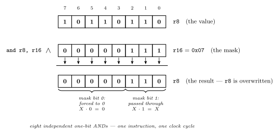
Figure 25: Why a mask works, one column at a time. Two rows of bits, an arrow down out of each column into a result row that overwrites the destination: here and r8, r16 with the mask 0x07, extracting the low three bits. The eight columns never interact — one mask bit decides one result bit, a 1 passing the value’s bit through and a 0 forcing it to zero — and all eight happen at once in a single instruction. Choosing a mask is therefore nothing more than deciding, position by position, which bits to keep.
Read Figure 25 column by column and the technique stops needing to be memorised: since the columns are independent, choosing a mask is just choosing, for each of the eight positions separately, whether that position gets passed through or forced.
The three identities that make it work
Each of AND, OR and XOR has a value that passes a bit through unchanged and a value that forces it. That pairing is the whole technique.
| \(X \cdot 0\) | \(X \cdot 1\) | \(X \cdot X\) | |
|---|---|---|---|
| AND | \(= 0\) | \(= X\) | \(= X\) |
| \(X + 0\) | \(X + 1\) | \(X + X\) | |
|---|---|---|---|
| OR | \(= X\) | \(= 1\) | \(= X\) |
| \(X \oplus 0\) | \(X \oplus 1\) | \(X \oplus X\) | |
|---|---|---|---|
| XOR | \(= X\) | \(= \overline{X}\) | \(= 0\) |
Reading off the pass-through and force columns gives the operation to reach for:
| To do this to the selected bits | Use | Mask bit = 1 on | Mask bit = 0 on |
|---|---|---|---|
| Clear them to 0 | AND |
the bits to keep — \(X \cdot 1 = X\) | the bits to clear — \(X \cdot 0 = 0\) |
| Set them to 1 | OR |
the bits to set — \(X + 1 = 1\) | everything else — \(X + 0 = X\) |
| Toggle them | EOR |
the bits to flip — \(X \oplus 1 = \overline{X}\) | everything else — \(X \oplus 0 = X\) |
| Extract them (others zeroed) | AND |
the bits to keep — \(X \cdot 1 = X\) | the bits to discard — \(X \cdot 0 = 0\) |
Note the asymmetry: AND’s mask is 1 on the bits you keep, whereas OR’s and XOR’s masks are 1 on the bits you act on. Getting that backwards is the usual bug — with AND you write the mask for what survives, with the other two for what changes.
\(X \oplus X = 0\) is the other one worth remembering: XORing a register with itself is the cheapest way to zero it.
In AVR assembly
The masks are ordinary constants, so the bitwise instructions of avr-instructions do the work. On AVR the immediate forms (andi, ori) only reach r16–r31; for a low register, load the mask into a high register and use the two-register form.
Extract the least significant three bits of r7 into r8, other bits of r8 zero.
    mov  r8, r7          ; copy the source
    ldi  r16, 0x07       ; mask 0000 0111 — keep the bottom three
    and  r8, r16         ; everything else forced to 0
Toggle the most significant four bits of r9, other bits unchanged.
    ldi  r16, 0xF0       ; 1111 0000 — flip the top four
    eor  r9, r16         ; bottom four XOR 0, so unchanged
Clear the least significant four bits of r10, other bits unchanged.
    ldi  r16, 0xF0       ; 1 on the bits to KEEP
    and  r10, r16        ; bottom four AND 0 -> 0
Set the most significant four bits of r11 to 1, other bits unchanged.
    ldi  r16, 0xF0       ; 1 on the bits to set
    or   r11, r16        ; bottom four OR 0, so unchanged
Note how 0xF0 appears as the mask in three of these with three different meanings — keep, flip, set — decided entirely by the instruction it is paired with.
In C
The same four operations with C’s bitwise operators (c-operators), which is how every AVR C program touches its ports. The masks are the same; the immediate-register restriction disappears, since the compiler chooses the registers.
| Operation | Operator | Example | Reads as |
|---|---|---|---|
| Clear particular bits | & with 0s on the bits to clear |
var = PINB & 0x0F; |
keep the low nibble, zero the high |
| Test particular bits | & with a 1 on the bit to test |
if (PINB & 0x02) … |
true if bit 1 is set |
| Set particular bits | \| with 1s on the bits to set |
PORTC = PINB \| 0x80; |
force bit 7 to 1 |
| Invert particular bits | ^ with 1s on the bits to flip |
PORTC = PINB ^ 0x0F; |
flip the low nibble |
Write the mask as a shift, not a hex constant: (1<<5) says bit 5 where 0x20 has to be decoded, and the header files name every register bit as a bit number for exactly this use (c-preprocessor-and-avr-headers):
DDRB  = (1<<5);                 /* bit 5 output, every other bit input: REPLACES the register */
DDRB |= (1<<4) | (1<<3);        /* bits 3 and 4 output, the rest unchanged: read-modify-write */
DDRB &= ~(1<<3);                /* bit 3 back to input, the rest unchanged                    */
PORTC ^= (1<<0);                /* toggle bit 0                                              */
TCCR1B = (1<<WGM12) | (1<<CS11) | (1<<CS10);   /* named bits, ORed into one value            */
The difference between the first two lines is the one that bites: = writes the whole register and silently sets the other seven bits to 0, |= ORs into what is already there. In assembly the second line is three instructions — in, ori, out — and the C compiler emits exactly those (week8-lab-avr-c-programming). For a single-bit clear the mask is the complement of the set mask, ~(1<<n), which is why clear bit 3 is &= ~(1<<3) and not &= (1<<3).
The test idiom needs no comparison. PINB & 0x02 is 0x02 when bit 1 is set and 0 when it is not, and C treats any non-zero value as true (c-control-flow) — so if (PINB & 0x02) is right and if ((PINB & 0x02) == 1) is always false, because the masked value is 2, never 1.
Set, clear and toggle on an I/O register
Changing one bit of an I/O register, and only that bit, is one of three lines. Each reads the register, combines it with a one-bit mask and writes it back:
| To | Write | The mask | Why the other bits survive |
|---|---|---|---|
| set bit n | REG \|= (1<<n); |
a 1 on bit n | \(X + 0 = X\) |
| clear bit n | REG &= ~(1<<n); |
a 0 on bit n, 1s elsewhere | \(X \cdot 1 = X\) |
| toggle bit n | REG ^= (1<<n); |
a 1 on bit n | \(X \oplus 0 = X\) |
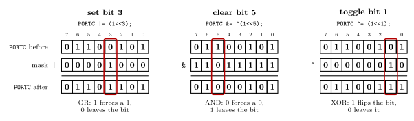
Figure 26: Set, clear and toggle on one register byte. Each panel starts from the same value of PORTC, 0110 0101, and changes one bit, outlined, with a single read-modify-write. The mask is a 1 shifted to the bit’s position, complemented for a clear. In every other column the mask holds the value that leaves a bit alone: 0 for OR and XOR, 1 for AND. Set gives 0110 1101, clear gives 0100 0101 and toggle gives 0110 0111, and each time the other seven bits are untouched.
Toggle is not enable. TIMSK2 ^= (1<<OCIE2A); turns the timer 2 compare A interrupt on only if it was off, and a second run turns it off again. To enable whatever the bit was before, set it with |=; to disable, clear it with &= ~. Toggling is for things meant to alternate, like an LED blinking.
The register has to be one that stores what is written. PORTx and DDRx do. PINx does not: it reads the pins, and on the ATmega324A a 1 written to one of its bits toggles the matching PORTx bit, so a read-modify-write on PINx changes the wrong bits (avr-io-ports).
Writing register bits by name
When setting or clearing bits of an I/O register, be explicit about which bits. Three ways to write the same value, from worst to best:
TCCR1B = 10;                          /* poor:   a number                    */
TCCR1B = 0x0A;                        /* better: the pattern, 0000 1010      */
TCCR1B = (1<<WGM12) | (1<<CS11);      /* best:   the bits, by name           */
WGM12 is bit 3 of TCCR1B and CS11 is bit 1, so all three are 0000 1010. Only the last says which bits, so a reader can check them against the datasheet without decoding anything: CTC mode, clock divided by 8 (avr-timers-and-counters). It costs nothing, either. The compiler works out (1<<WGM12) | (1<<CS11) while compiling, and all three lines become the same instructions.
The names are bit numbers. The device header that <avr/io.h> includes defines every bit name as the bit’s position in its register:
#define WGM02 3A name is not a mask; 1<< makes it one (c-preprocessor-and-avr-headers). The names are the datasheet’s, and the datasheet has errors in places, so the I/O register summary at the back is the one to check a name against.
Assembly uses the same names. In ldi r16, (1<<WGM02)|(1<<CS01) the assembler works out the constant, 0x0A, and the instruction stored is ldi r16, 0x0A.
A name belongs to one register. WGM12 and WGM02 are both 3, so (1<<WGM12) written into TCCR0B sets WGM02, and the compiler cannot notice, because all it sees is the number 3. Pair each name with the register whose datasheet entry defines it. The same byte 0x0A is CTC mode in TCCR1B and a reserved mode in TCCR0B (2026-10-05-more-io).
Masking sets the status flags too
Status register flags will be set also — a mask operation is a real ALU operation, not a free one. AND, OR and EOR all clear V and set N and Z from the result (C is untouched); see avr-architecture.
That side effect is often the actual point. andi r16, 0x01 keeps only bit 0, so:
\[Z = 1 \iff \text{bit 0 of } \texttt{r16} \text{ is } 0 \iff \texttt{r16} \text{ is even}\]
which makes a single masked AND an even/odd test. Any single-bit mask turns the Z flag into a test of that one bit — and tst rd, which is just and rd, rd, is the degenerate case that tests the whole register against zero.
Common mistakes
&= (1<<n)to clear bit n. That keeps bit n and clears the other seven. A clear’s mask is the complement,~(1<<n).=where|=was meant.DDRB = (1<<5)makes PB5 an output and every other pin of port B an input.- A bit name without the shift.
TCCR1B |= WGM12;ORs in the number 3,0000 0011, which setsCS11andCS10, clock divided by 64, and leavesWGM12alone. - A bit name in the wrong register.
(1<<WGM12)inTCCR0BsetsWGM02. ^=to enable. A toggle enables only from off; run twice, it disables.- A read-modify-write on
PINx. WritingPINxtoggles outputs, so it cannot clear or set a bit. - Getting AND’s mask backwards. With AND the 1s mark the bits to keep; with OR and XOR they mark the bits to change.
if ((x & mask) == 1). The masked value is the mask’s own value, so the test is false unless the mask is bit 0. Test for non-zero.
See also
- boolean-algebra · avr-instructions · avr-architecture
- avr-io-ports — one bit of a port in C and assembly, and why
PINxis different - avr-timers-and-counters — the
TCCRnBfields named in the examples - 2026-10-05-more-io — Lecture 19: poor, better and best,
TIMSK2toggled - week5-lab-avr-assembly-one — Lab 9, where these snippets are the exercise
- week8-lab-avr-c-programming — Lab 11, the same operations in C · c-operators · c-preprocessor-and-avr-headers
Boolean Algebra
Logic functions can be expressed as expressions of variables (literals, e.g. \(A, B, X\)) and functions (the operators \(+\), \(\cdot\), \(\oplus\), \(\bar{\ }\)) — i.e. an output written in terms of its inputs, \(X = f(A,B)\). Variables and functions can only take the values 0 or 1. Boolean algebra is the set of rules governing how such expressions can be manipulated.
Notation conventions
- Inversion: overline, e.g. \(\text{NOT}(A) = \bar A\) (pronounced “A bar”).
- AND: dot, or implied by adjacency, e.g. \(\text{AND}(A,B) = AB = A \cdot B\).
- OR: plus sign, e.g. \(\text{OR}(A,B,C) = A+B+C\).
- Other examples: \(\text{XOR}(A,B) = A \oplus B = \bar A B + A \bar B\); \(\text{NAND}(A,B,C) = \overline{ABC}\); \(\text{NOR}(A,B) = \overline{A+B}\).
\(+\) and \(\cdot\) are OR and AND, not arithmetic addition and multiplication — \(1 + 1 = 1\) here.
Boolean identities
| Name | AND form | OR form |
|---|---|---|
| Identity law | \(1A = A\) | \(0 + A = A\) |
| Null law | \(0A = 0\) | \(1 + A = 1\) |
| Idempotent law | \(AA = A\) | \(A + A = A\) |
| Inverse law | \(A\bar A = 0\) | \(A + \bar A = 1\) |
| Commutative law | \(AB = BA\) | \(A + B = B + A\) |
| Associative law | \((AB)C = A(BC)\) | \((A+B)+C = A+(B+C)\) |
| Distributive law | \(A + BC = (A+B)(A+C)\) | \(A(B+C) = AB + AC\) |
| Absorption law | \(A(A+B) = A\) | \(A + AB = A\) |
| De Morgan’s law | \(\overline{AB} = \bar A + \bar B\) | \(\overline{A+B} = \bar A \bar B\) |
Two rows in particular do the heavy lifting when simplifying: the inverse law (\(A\bar A = 0\), \(A + \bar A = 1\)) collapses whole terms to a constant, and the absorption law (\(A + AB = A\)) deletes a term outright.
The distributive law in its AND form is not the arithmetic one — \(A + BC = (A+B)(A+C)\) has no algebraic analogue and is easy to misremember.
De Morgan’s law and gate equivalents
De Morgan’s law says AND and OR can be interchanged if you invert both the inputs and the output. Drawn as gates, that gives four equivalences — every gate has a second symbol, and pushing an inversion through a gate always flips its shape:
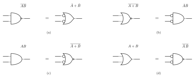
Figure 27: De Morgan’s law drawn as gate symbols. (a) a NAND is an OR with inverted inputs; (b) a NOR is an AND with inverted inputs; (c) and (d) are the same two statements read the other way. Each pair is the same function, so either symbol may be used - pick whichever makes the surrounding bubbles cancel.
Exercise: verify each of the four with a truth table.
This is also why NAND-only and NOR-only circuits can implement any function (see logic-gates) — an AND feeding an OR can always be redrawn as a NAND feeding a NAND.
Simplifying an expression
Worked example:
\[\text{CODE} = C + CD + \overline{(D + \bar D)}\]
- Apply De Morgan’s law to the last term: \(\overline{D + \bar D} = \bar D \cdot \bar{\bar D} = \bar D \cdot D = 0\) (the double overline cancels, then the inverse law \(A\bar A = 0\) applies).
- The identity law \(0 + A = A\) drops that term: \(\text{CODE} = C + CD\).
- The absorption law \(A + AB = A\) finishes it: \(\text{CODE} = C\).
The whole expression is just \(C\) — neither \(D\) nor the \(CD\) term affects the output at all.
Sum of products
Any logic function can be implemented as the OR of AND combinations of its inputs (a sum of products):
- For each row where the truth table output is 1, write the AND term of the inputs (complementing wherever the input is 0) that produces that row.
- OR all of those terms together.
Because every 1-row gets its own term, and each term is true for exactly that one row, the result is guaranteed to reproduce the table. Worked through in full, with the resulting circuit drawn out, in 2026-07-30-intro-to-logic-gates.
Sum of products always works, but does not necessarily give the minimum number of gates — the resulting expression can usually be simplified further with the identities above. E.g. \(Z = AB + AC = A(B+C)\) (distributive law) needs two gates rather than three.
Circuit Schematics
A logic diagram shows the idea of a circuit and is hardware-independent (see logic-gates). A circuit schematic goes further: it tells you how to actually build the circuit on real hardware — labelled ICs, pin numbers, power connections — so it’s hardware-specific. Schematics are drawn for practicals and assessment using 74-series logic chips and the CSSE2010/CSSE7201 IO Board (see device-pinouts for pin layouts). The rules are set out in the CSSE2010/CSSE7201 - Guide to Drawing Circuit Schematics (Blackboard, v2.3).
Required elements
Every circuit schematic must show:
- Labelled inputs and outputs — every input/output needs a sensible, unique name. Inputs and outputs use different symbols, and by convention inputs are drawn on the left, outputs on the right.
- Both symbols are the same right-pointing pentagon; what differs is which end the wire attaches to. An input has its wire leaving the point, so the signal flows out of the tip into the circuit. An output has its wire arriving at the flat back edge, with the point left free. Getting this backwards is one of the common errors below.
- Labelled devices — each physical device (chip or IO board) gets a unique identifier: one or more letters for the device type, then a sequential number starting from 1.
- Logic chips:
U1,U2,U3, … - IO board:
IO1(IO2for a second board, etc.) — when a group of inputs/outputs all belong to the same IO board, it only needs to be labelled once for the whole group, not per signal.
- Logic chips:
- Gate labels within a chip — where a chip contains multiple gates, each gate is labelled
A,B,C, … after the chip ID, separated by a colon (e.g.U1:A,U1:B). Labels can be assigned to gates in any order. A chip with only one gate/device doesn’t need a gate letter (justU3). - Device type — written on the line below the device ID (e.g.
74HCT00,74HCT04,IOBOARD). - Pin numbers — every pin used must be numbered per the actual device pinout (see device-pinouts).
- Power supply connections — shown once per device type, not per individual chip. Where two+ chip types share the same power pins, they can be grouped together. The IO board doesn’t need power connections shown.
Worked example
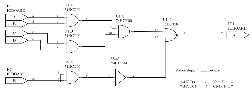
Figure 28: A correct schematic. Every rule above is visible here at once: five named inputs (A-E) and one named output (X0) on the IO board, four gates of one 74HCT00 labelled U1:A to U1:D, a fifth NAND that had to move to a second chip U2, an inverter on a third chip U3 because it is a different gate type, a pin number on every terminal, a junction dot where E splits to both inputs of U2:A, and one power-supply block covering both chip types.
Reading it against the rules:
- Naming: the inputs are
A,B,C,D,Eand the output isX0. The two IO-board groups are each labelledIO1/IOBOARDonce, not per signal. - Chip identifiers:
U1supplies four NAND gates (U1:A–U1:D). A fifth NAND is needed, so it comes from a second chip,U2:A. The inverter is a different gate type, so it needs a third chip,U3:A, of type 74HCT04. - Pin numbers: the 74HCT00’s four gates use inputs 1&2, 4&5, 9&10, 12&13 with outputs 3, 6, 8, 11 respectively — so those are the numbers written on
U1:A–U1:D.U3:Auses 1 → 2. - The junction dot:
E(pin 25) drives both inputs ofU2:A, which is what turns a NAND into an inverter. The dot at the split is what says the two wires are joined. - Power:
74HCT00and74HCT04have the same power pins, so they are braced together into one block: Vcc on pin 14, GND on pin 7. Nothing is shown per chip, and nothing at all for the IO board.
Common errors
Figure 29: The same circuit with seven deliberate mistakes ringed and numbered left to right, matching the list below. Compare each ring against the corresponding part of the correct schematic above.
- Duplicate names — two inputs given the same name (both called
A). Every input needs a unique name. - Missing junction dots — where wires join or split, a dot must mark the connection. Wires that merely cross on the page, with no dot, are not electrically connected. Here the split feeding both inputs of the NAND-as-inverter has no dot.
- Gate label exceeds chip capacity —
U1:Eon a 74HCT00, which only has four 2-input NAND gates (A–D). A fifth gate needs a new chip ID (U2:Aor similar). - Wrong device for the gate type —
U1:Fis a NOT gate, a different type from the rest ofU1, so it needs its own chip identifier (U3:A). (The figure also gives it as a74LS04while the rest of the schematic uses74HCTparts.) - Reusing pin numbers —
U1:Cis drawn with pins 1, 2 → 3, the same physical gate asU1:A. You can’t use one gate twice. - Inconsistent device type —
U1:Dis labelled74HCT47when the rest ofU1is a74HCT00. Every gate labelledU1:somethingmust show the same chip type. - Output errors — two distinct mistakes on
X0:- The input symbol is used (wire attached to the point) where the output symbol is needed (wire attached to the flat back) — see Figure 28.
- An input is wired to the output of a gate. An input should never be tied straight to a gate’s output; this may destroy the device. Gate outputs should only feed output devices (e.g. LEDs) or the inputs of other gates.
See also
- device-pinouts — the pin numbers and symbols every schematic has to match
- logic-gates — the gate symbols themselves, and the logic-diagram level above this one
- week3-lab-lab-4-pre-work — the preparation task that asks for schematics of a 2-to-1 mux, a 2-to-4 decoder and a 4-bit adder/subtractor
Combinational Logic Blocks
Reference note for the standard combinational building blocks: the adder-subtractor, the multiplexer, and the decoder. See logic-gates for the gate symbols/truth tables and boolean-algebra for the notation used below.
What makes a circuit combinational
A combinational circuit is a combination of logic gates with \(n\) inputs and \(m\) outputs:
- Each output can be expressed as a function of the \(n\) input variables.
- The output depends on the current inputs only — there is no memory of previous inputs. (Contrast with sequential-circuits, where the output also depends on stored state.)
- It can always be written as a truth table with \(n\) input columns, \(m\) output columns, and \(2^n\) rows (one per possible input combination).
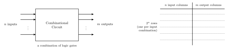
Figure 30: The general shape of a combinational circuit and the truth table it is always equivalent to. The row count \(2^n\) depends only on the number of inputs, and the output column count \(m\) only on the number of outputs — so a block with six inputs needs 64 rows however few gates are inside it.
Binary subtraction
\(A - B\) is usually implemented as \(A + (-B)\), where:
- \(A\) and \(B\) are multi-bit quantities;
- “+” here means addition, not OR;
- \(-B\) means the two’s complement of \(B\) (see binary-number-representations).
The two’s complement of \(B\) is calculated by flipping all the bits and adding 1:
\[-B = \bar B + 1\]
So a subtractor is just an adder with two extra pieces: something that conditionally inverts \(B\), and something that adds the extra 1.
The controlled inverter (XOR trick)
We need a gate that flips a bit only sometimes: given a mode bit \(M\),
\[Z = \bar B \text{ when } M = 1, \qquad Z = B \text{ when } M = 0\]
From the XOR truth table: XOR with one input held at 0 passes the other input through unchanged, and XOR with one input held at 1 inverts it. So the gate is a 2-input XOR:
\[Z = B \oplus M\]
| M | B | \(Z = B \oplus M\) | Effect |
|---|---|---|---|
| 0 | 0 | 0 | pass through |
| 0 | 1 | 1 | pass through |
| 1 | 0 | 1 | invert |
| 1 | 1 | 0 | invert |

Figure 31: The controlled inverter: one XOR gate per bit, with the mode line on the second input. The two identities on the right are the whole trick, and they hold for any signal X — XOR against a constant 0 is a wire, XOR against a constant 1 is an inverter.
This is called a controlled inverter.
Adder-subtractor circuit
A 4-bit adder-subtractor is built from a 4-bit binary adder (a ripple-carry adder — see 2026-08-04-binary-arithmetic) plus four XOR gates:
- Data input \(A\) (\(A_0 \ldots A_3\)) goes straight into the adder’s \(A\) inputs.
- Data input \(B\) (\(B_0 \ldots B_3\)) goes into the adder’s \(B\) inputs via one XOR gate per bit; the second input of every XOR gate is the shared mode select line \(M\).
- \(M = 0\) means add, \(M = 1\) means subtract.
- The adder produces the data output \(S_0 \ldots S_3\), plus a carry-out \(C_4\) and taking a carry-in \(C_0\).
The carry-in. With \(M = 1\) the XOR gates supply \(\bar B\), and two’s complement needs \(\bar B + 1\) — the extra \(+1\) is supplied by feeding it in as the carry-in. With \(M = 0\) we want plain addition, which needs a carry-in of 0. Both cases are satisfied by
\[C_0 = M\]
so the mode select line is wired to both the XOR gates and the adder’s carry-in.
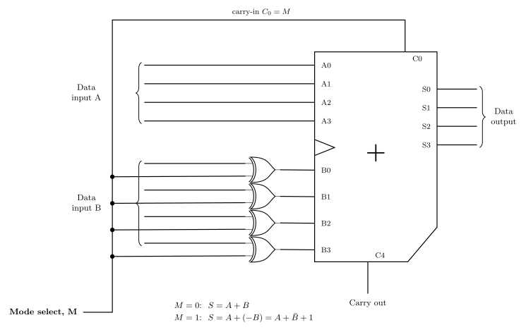
Figure 32: The 4-bit adder-subtractor. One mode line does two jobs: it conditions every bit of B through an XOR, and it is the adder’s carry-in. With M = 0 the XORs pass B through and the carry-in is 0, so the adder computes A + B; with M = 1 the XORs deliver B-bar and the carry-in is 1, so it computes A + B-bar + 1, which is A + (-B). No extra hardware is spent on the +1 at all.
The cost of subtraction is therefore four XOR gates and one wire on top of an adder — a 74HCT86 (quad 2-input XOR) plus a 74HCT283 (4-bit adder), see device-pinouts.
Multiplexer (mux)
A multiplexer — also called a data selector — has:
- \(2^n\) data inputs,
- 1 output,
- \(n\) control (or select) inputs, which select one of the data inputs to be “sent” or “steered” to the output.
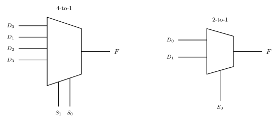
Figure 33: The multiplexer logic symbol at two sizes, 4-to-1 and 2-to-1. Data inputs enter the tall left edge, the single output leaves the short right edge, and the select inputs enter from underneath. The number of select lines is what fixes the size: n selects steer 2^n data inputs.
4-to-1 multiplexer
Data inputs \(D_0 \ldots D_3\), select inputs \(S_1 S_0\), output \(F\). The logic symbol is the characteristic trapezoid with the data inputs on the wide (left) edge, \(F\) on the narrow (right) edge, and the select inputs entering the bottom.
Function table:
| \(S_1\) | \(S_0\) | \(F\) |
|---|---|---|
| 0 | 0 | \(D_0\) |
| 0 | 1 | \(D_1\) |
| 1 | 0 | \(D_2\) |
| 1 | 1 | \(D_3\) |
This is a function table, not a full truth table — the full truth table would need \(2^6 = 64\) rows for the six inputs \(S_1, S_0, D_0, D_1, D_2, D_3\). The function table’s four rows say the same thing far more compactly, which is why it is what gets drawn.
4-to-1 mux logic circuit implementation
- \(S_1\) and \(S_0\) each feed an inverter, giving \(\bar S_1\) and \(\bar S_0\) as well as the true forms.
- Four 3-input AND gates, one per data input. Each AND gate takes its data input plus the select-literal pair that identifies it: \(D_0\) with \(\bar S_1 \bar S_0\), \(D_1\) with \(\bar S_1 S_0\), \(D_2\) with \(S_1 \bar S_0\), \(D_3\) with \(S_1 S_0\).
- The four AND outputs feed a single 4-input OR gate whose output is \(F\).
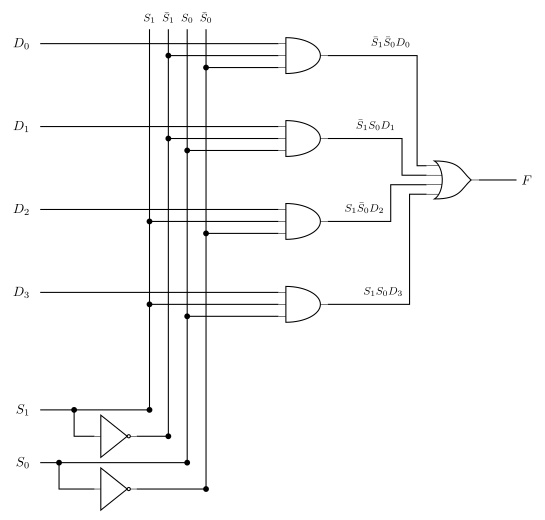
Figure 34: A 4-to-1 multiplexer built from gates. The two inverters generate the complemented selects; the four vertical rails carry S1, S1-bar, S0 and S0-bar past every AND gate; each AND gate is one data input gated by the one select combination that names it, and the OR gate collects them. Only the dots are connections — every other crossing is two wires passing.
That is exactly the sum-of-products form:
\[F = D_0 \bar S_1 \bar S_0 + D_1 \bar S_1 S_0 + D_2 S_1 \bar S_0 + D_3 S_1 S_0\]
Only the AND gate whose select literals match the current \(S_1 S_0\) can be 1, so exactly one data input reaches the OR gate at a time. The other three AND gates output 0, and \(0\) is the identity for OR, so they contribute nothing.
The gate-level version needs 3-input ANDs and a 4-input OR, neither of which exists in the lab kit (see device-pinouts) — building this from the available 2-input chips means cascading them.
2-to-1 multiplexer
Data inputs \(D_0\) and \(D_1\), one control input \(S_0\), output \(F\).
Function table:
| \(S_0\) | \(F\) |
|---|---|
| 0 | \(D_0\) |
| 1 | \(D_1\) |
Expanded to a full truth table over all three inputs (\(2^3 = 8\) rows):
| \(S_0\) | \(D_0\) | \(D_1\) | \(F\) |
|---|---|---|---|
| 0 | 0 | 0 | 0 |
| 0 | 0 | 1 | 0 |
| 0 | 1 | 0 | 1 |
| 0 | 1 | 1 | 1 |
| 1 | 0 | 0 | 0 |
| 1 | 0 | 1 | 1 |
| 1 | 1 | 0 | 0 |
| 1 | 1 | 1 | 1 |
i.e. \(F = D_0 \bar S_0 + D_1 S_0\). When \(S_0 = 0\) the output tracks \(D_0\) and ignores \(D_1\); when \(S_0 = 1\) it tracks \(D_1\) and ignores \(D_0\).
A quad 2-input multiplexer is available as an off-the-shelf IC — the 74HCT157, see device-pinouts.
Using a mux to implement a logic function
Because the data inputs can be tied to constant 0 or 1, an \(n\)-select mux with its selects wired to the function’s variables can implement any function of those \(n\) variables: set data input \(D_i\) to the value the function should take when the selects equal \(i\). The function table is the truth table of the function, read off directly. See the worked question in 2026-08-06-combinational-logic.
Decoder
A decoder converts an \(n\)-bit input to a logic 1 on exactly one of its \(2^n\) outputs (the one whose index equals the input value); all other outputs are 0.
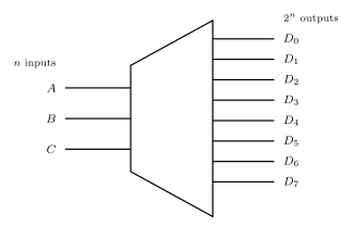
Figure 35: The decoder as a block: n inputs in, 2^n outputs out, and the shape widens accordingly. It is the mux’s opposite — a mux funnels 2^n inputs down to one output under n selects, a decoder fans n inputs out to 2^n outputs.
3-to-8 decoder
Inputs \(A, B, C\) (with \(A\) the most significant), outputs \(D_0 \ldots D_7\).
| A | B | C | \(D_0\) | \(D_1\) | \(D_2\) | \(D_3\) | \(D_4\) | \(D_5\) | \(D_6\) | \(D_7\) |
|---|---|---|---|---|---|---|---|---|---|---|
| 0 | 0 | 0 | 1 | 0 | 0 | 0 | 0 | 0 | 0 | 0 |
| 0 | 0 | 1 | 0 | 1 | 0 | 0 | 0 | 0 | 0 | 0 |
| 0 | 1 | 0 | 0 | 0 | 1 | 0 | 0 | 0 | 0 | 0 |
| 0 | 1 | 1 | 0 | 0 | 0 | 1 | 0 | 0 | 0 | 0 |
| 1 | 0 | 0 | 0 | 0 | 0 | 0 | 1 | 0 | 0 | 0 |
| 1 | 0 | 1 | 0 | 0 | 0 | 0 | 0 | 1 | 0 | 0 |
| 1 | 1 | 0 | 0 | 0 | 0 | 0 | 0 | 0 | 1 | 0 |
| 1 | 1 | 1 | 0 | 0 | 0 | 0 | 0 | 0 | 0 | 1 |
The 1 always sits in the column whose index is the binary value of \(ABC\).
Each row of the table is one minterm: the top row is \(\bar A \bar B \bar C\) and the bottom row is \(ABC\).
3-to-8 decoder logic circuit implementation
- Each of \(A\), \(B\), \(C\) is fanned out to an inverter, so all six literals \(A, \bar A, B, \bar B, C, \bar C\) are available on a vertical bus.
- Eight 3-input AND gates, one per output. Each taps the three literals matching its index:
\[D_0 = \bar A \bar B \bar C, \quad D_1 = \bar A \bar B C, \quad D_2 = \bar A B \bar C, \quad D_3 = \bar A B C\] \[D_4 = A \bar B \bar C, \quad D_5 = A \bar B C, \quad D_6 = A B \bar C, \quad D_7 = ABC\]
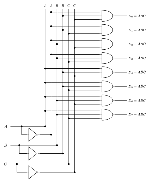
Figure 36: A 3-to-8 decoder built from gates. Three inverters generate the complements onto six vertical rails; each of the eight AND gates taps the one literal triple that matches its index, so it is the minterm for that input combination. Exactly one AND gate can be high at a time, which is the decoder’s defining property.
Each AND gate is the minterm for one input combination, so exactly one is high at any time.
Using a decoder to implement a logic function
Because a decoder hands you every minterm of its inputs on a separate wire, any function of those inputs is just an OR of the minterm outputs whose truth-table rows are 1. For example, take
\[F = \bar A \bar B \bar C + ABC\]
which is \(D_0 + D_7\) — one OR gate on two decoder outputs, with nothing else needed.
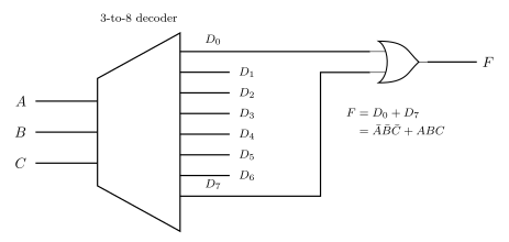
Figure 37: A function built on a decoder: F = A-bar B-bar C-bar + ABC is D0 + D7, so it costs a single OR gate on top of the decoder. Any function of A, B and C can be built this way — pick out the outputs for its true rows and OR them together.
This is the same idea as the mux trick above, approached from the other side: a mux picks one of \(2^n\) values, a decoder hands you all \(2^n\) minterms and you OR the ones you want.
See also
- 2026-08-06-combinational-logic — Lecture 4, where these blocks were introduced
- device-pinouts — the off-the-shelf parts: 74HCT157 (mux), 74HCT283 (adder), 74HCT86 (XOR)
- arithmetic-logic-unit — the ALU bit slice, which is a mux selecting between several function blocks
- binary-number-representations — two’s complement, on which the subtractor depends
Counters
A counter is a multi-bit register that goes through a determined sequence of states (values) upon the application of input (clock) pulses. It is a synchronous sequential circuit built from D flip-flops plus some combinational logic in the feedback path.
Binary counters
A counter which follows the binary number sequence is a binary counter.
An \(n\)-bit binary counter:
- has \(n\) flip-flops;
- has \(2^n\) different states;
- counts from \(0\) to \(2^n - 1\), then wraps back to \(0\).
For example, a 2-bit binary counter counts
\[00 \to 01 \to 10 \to 11 \to 00 \to \ldots\]
i.e. \(0 \to 1 \to 2 \to 3 \to 0 \to \ldots\)
4-bit binary counter — counting sequence
| Bit 3 | Bit 2 | Bit 1 | Bit 0 | Value |
|---|---|---|---|---|
| 0 | 0 | 0 | 0 | 0 |
| 0 | 0 | 0 | 1 | 1 |
| 0 | 0 | 1 | 0 | 2 |
| 0 | 0 | 1 | 1 | 3 |
| 0 | 1 | 0 | 0 | 4 |
| 0 | 1 | 0 | 1 | 5 |
| 0 | 1 | 1 | 0 | 6 |
| 0 | 1 | 1 | 1 | 7 |
| 1 | 0 | 0 | 0 | 8 |
| 1 | 0 | 0 | 1 | 9 |
| 1 | 0 | 1 | 0 | 10 |
| 1 | 0 | 1 | 1 | 11 |
| 1 | 1 | 0 | 0 | 12 |
| 1 | 1 | 0 | 1 | 13 |
| 1 | 1 | 1 | 0 | 14 |
| 1 | 1 | 1 | 1 | 15 |
| 0 | 0 | 0 | 0 | 0 |
Each bit toggles at half the rate of the bit to its right — bit 0 changes every count, bit 1 every second count, bit 2 every fourth, bit 3 every eighth.
Key points
- The next state is a function of the present state (and possibly of external inputs).
- The count sequence can be the binary numbers but does not have to be — if it is, the counter is a binary counter; otherwise it is just some arbitrary cycle through states.
- These circuits are synchronous: all flip-flops share the same clock.
- Asynchronous counters exist too, but are not discussed in this course.
State: the design idea
This is the whole trick, and it is what makes counter design mechanical:
- The values stored in the flip-flops are the current (present) state of the circuit.
- The \(D\) inputs to the flip-flops are the next state — whatever is sitting on \(D\) at the clock edge becomes the new state.
- The \(D\) inputs are some combinational function of the current state (and of any external inputs).
So for a counter with state bits \(Q_{n-1} \ldots Q_1 Q_0\), designing the counter means finding \(n\) Boolean expressions
\[D_i = f_i(Q_{n-1}, \ldots, Q_1, Q_0)\]
and building each one out of gates.
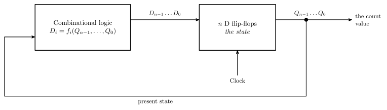
Figure 38: A counter is the general sequential-circuit block diagram with the external inputs deleted. That diagram, as Mano draws it, is a combinational circuit feeding flip-flops, the flip-flop outputs routed back round to the combinational circuit, and the clock entering the flip-flops on its own labelled stub. A counter may or may not have external inputs; removing them, as here, is what makes the design mechanical: with nothing else to depend on, each D is a function of the Q values alone, so the present-state/next-state table below is a complete specification of the circuit.
Design recipe
- Write down the count sequence you want, as a cycle of state values.
- Build a present-state / next-state table. One row per possible state — all \(2^n\) of them, not just the ones in your sequence. Columns: present state \(Q_{n-1}\ldots Q_0\), then next state \(D_{n-1}\ldots D_0\). Fill each next-state entry by reading off what follows that state in your sequence.
- Handle unused states. If your sequence doesn’t use all \(2^n\) states, the next state for the unused ones is a don’t-care (X). You may set each X to whatever makes the algebra simplest — but check afterwards where the unused state actually goes, because a self-correcting counter (one whose unused states lead back into the cycle) is nicer than one that can get stuck.
- Read each \(D\) column as a Boolean function of the \(Q\)s. The table is a truth table with the \(Q\)s as inputs and \(D_i\) as the output, so write it in sum-of-products form: OR together one AND term per row where \(D_i = 1\). See boolean-algebra.
- Simplify each expression using the Boolean algebra laws (and the don’t-cares), then draw the circuit: the combinational logic for \(D_i\) feeding flip-flop \(i\), with every flip-flop on a common clock. See circuit-schematics for schematic conventions and device-pinouts for the 74HCT74 / 74HCT175 D flip-flop packages.
The smallest case falls straight out of the recipe: a 1-bit counter counts \(0 \to 1 \to 0 \to \ldots\), so its next state is always the complement of its present state, giving \(D = \bar Q\) — a single flip-flop with its \(\bar Q\) output wired back to its own \(D\) input (a toggle).
Worked example — a 2-bit counter for \(00 \to 10 \to 01 \to 00\)
Step 1–2 — present-state / next-state table. The sequence uses three of the four states; \(11\) is unused, so its next state is a don’t-care.
| \(Q_1\) | \(Q_0\) | \(D_1\) | \(D_0\) | comment |
|---|---|---|---|---|
| 0 | 0 | 1 | 0 | \(00 \to 10\) |
| 0 | 1 | 0 | 0 | \(01 \to 00\) |
| 1 | 0 | 0 | 1 | \(10 \to 01\) |
| 1 | 1 | X | X | unused state |
Step 4 — read off the columns.
\(D_1\) is 1 only in the row \(Q_1Q_0 = 00\). Making the don’t-care 1 would give \(Q_1 \odot Q_0\) (XNOR), which is no simpler, so take the don’t-care as 0 (\(X_1 = 0\)):
\[D_1 = \bar Q_1 \bar Q_0\]
\(D_0\) is 1 only in the row \(Q_1Q_0 = 10\), which gives \(D_0 = Q_1\bar Q_0\). Here the don’t-care does help: setting it to 1 (\(X_0 = 1\)) makes \(D_0 = 1\) for both rows with \(Q_1 = 1\), so
\[D_0 = Q_1\]
Step 5 — the circuit. Two D flip-flops on a common clock. Flip-flop 0’s \(D\) input is wired directly to flip-flop 1’s \(Q_1\) output — no gate at all. Flip-flop 1’s \(D\) input is driven by a 2-input NOR of \(Q_1\) and \(Q_0\) (since \(\bar Q_1 \bar Q_0 = \overline{Q_1 + Q_0}\)), or equivalently by an AND of the two \(\bar Q\) outputs.
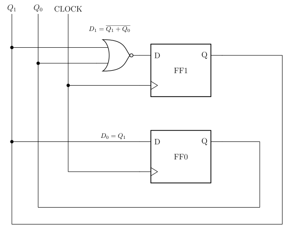
Figure 39: The whole counter, drawn from the derivation above. Each Q runs back to a vertical rail that the next-state logic taps, which is the physical form of the feedback loop in the block diagram earlier: D0 is FF1’s Q wired straight across with no gate at all, and D1 is one NOR gate. Dots are connections; where the Q0 rail and the CLOCK rail cross the D0 wire there is no dot and no connection. The circuit takes the NOR form of D1; an AND of the two Q-bar outputs is the same function and would need the flip-flops’ Q-bar pins instead.
Check, including the unused state:
| present | \(D_1 D_0\) | next |
|---|---|---|
| 00 | 1 0 | 10 |
| 10 | 0 1 | 01 |
| 01 | 0 0 | 00 |
| 11 | 0 1 | 01 |
The cycle is right, and the unused state falls into the cycle on the next clock edge, \(11 \to 01\), so the counter is self-correcting — a robust design. (Choosing \(D_0 = Q_1\bar Q_0\) instead — don’t-care set to 0 — would send \(11 \to 00\), also fine, at the cost of a whole extra gate: an AND fed from \(Q_1\) and the flip-flop’s \(\bar Q_0\) pin, where \(D_0 = Q_1\) needs no gate at all.)
Applied exercise
week4-lab-lab-7-exercises is exactly this recipe at \(n = 3\): design a 3-bit synchronous counter that steps through an allocated 7-state sequence, with the eighth (missing) state treated as a don’t-care.
CPU Organisation
Where the digital logic of the first half of the course ends up: the blocks a processor is made of, and what each one holds. See arithmetic-logic-unit for the ALU in detail and fetch-decode-execute-cycle for what the control unit does with all of it.
Computer organisation
A simplified view of a whole machine: a CPU connected by external buses to main memory, secondary storage and IO devices, with internal buses wiring together the CPU’s own blocks.
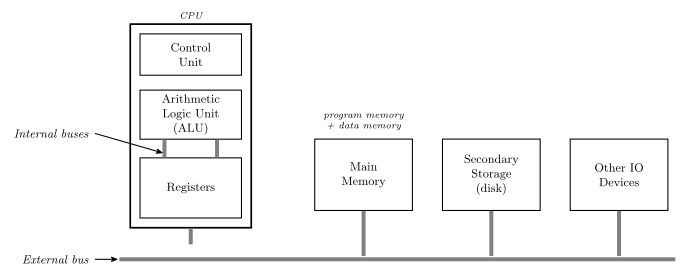
Figure 40: Simplified computer organisation. The CPU’s three blocks are joined by internal buses; a single external bus carries everything between the CPU and the rest of the machine. Main memory holds both the program and the data operated on, so it is both program memory and data memory.
Main memory holds both the program and the data: the instructions to be fetched and the values to be operated on.
Parts of a CPU
| Block | Role |
|---|---|
| Control Unit | Fetches instructions from memory, and makes the ALU and the registers perform the instruction |
| ALU | Performs arithmetic and logical operations |
| Registers | High-speed memory — stores temporary results and control information |
How many registers, and how wide, varies enormously with the machine: a small CPU may have 8 × 8-bit registers, a large one 64 × 32-bit registers. The AVR used later in this course has 32 registers (R0–R31) and an 8-bit word, so it also has an 8-bit ALU.
Registers
Registers are temporary storage locations inside the CPU. Two types:
General purpose registers hold the data to be operated on (e.g. data read from memory) and the results of operations. Collectively they are the register file, and their width is the CPU word size.
Special purpose registers are used by the system rather than by the program’s arithmetic:
| Register | Holds |
|---|---|
| Program Counter (PC) | the address of the next instruction to be fetched from memory |
| Instruction Register (IR) | the current instruction |
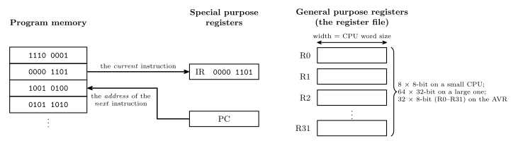
Figure 41: The two types of register, and why the distinction matters. A general purpose register is one anonymous row of the file, as wide as the machine word and picked by number; a special purpose register is named, and what it holds is interpreted — the PC as an address into program memory, the IR as an instruction to be decoded. The particular bit patterns shown in memory are illustrative only.
A third special purpose register, the status register, records what the last ALU operation did — see fetch-decode-execute-cycle. PC and IR are the two the fetch step manipulates directly.
See also
- arithmetic-logic-unit · fetch-decode-execute-cycle
- binary-number-representations — word sizes and two’s complement, which fix what the registers can hold
- avr-architecture — the same three blocks as an actual chip
- memory-hierarchy-and-cache — the registers at the top of the memory hierarchy, and the cache between the CPU and main memory
- 2026-08-24-alu-and-control-unit — Lecture 9
CSSE2010 Diagram Notation
The drawing conventions this course actually uses, inferred from its own materials. This is the reference every later diagram in CSSE2010 should be checked against.
Scope. This note covers the diagram families that the two existing notation notes do not: gate symbols and logic diagrams, timing/waveform diagrams, state diagrams and state tables, block and datapath diagrams, register/memory layout diagrams, and the AVR architecture figures. It also records the algebraic and textual notation the figures depend on. For circuit-schematic rules (device IDs, gate letters, pin numbers, junction dots, power blocks, IO-board input/output pentagons) see circuit-schematics; for the 74-series pinouts and their schematic symbols see device-pinouts. Those two are not repeated here.
What was read
An honest statement of the sample, because most of what follows is inferred from drawings rather than stated in prose.
Guides — all three read in full (9 of 9 pages):
- CSSE2010/CSSE7201 Device Pinouts and Symbols (v4), pp. 1–2
- CSSE2010/CSSE7201 — Guide to Drawing Circuit Schematics (v2.3, Semester One 2016), pp. 1–2
- I/O Board User Manual, pp. 1–5
Lecture decks — 221 of 246 pages:
| Deck | Pages read | of |
|---|---|---|
| L01 Intro and Binary Numbers | 1–20 | 21 |
| L02 Intro to Logic Gates | 1–24 | 24 |
| L03 Binary Arithmetic | 8–17 | 17 |
| L04 Combinational Logic | 1–19 | 19 |
| L05 Flip-Flops | 4–19 | 19 |
| L06 Shift Registers | 3–17 | 17 |
| L07 Counters | 3–17 | 17 |
| L08 State Machines | 2–21 | 21 |
| L09 ALU and Control Unit | 3–22 | 22 |
| L10 AVR Introduction | 3–19 | 19 |
| L11 ISA Part 1 | 3–28 | 28 |
| L12 ISA Part 2 | 2–20 | 22 |
Unread: L01 p21, L03 pp1–7, L05 pp1–3, L12 pp21–22 — title, outline and admin pages in every case except L03 pp1–7 (number-representation recap, no new diagram family). Labs, past papers and the course profile were not sampled at all.
Citation format below: “L04 s10” means lecture deck 04, slide 10. Slide numbers printed on the slides match the PDF page numbers in every deck checked.
The course ships no notation guide for these diagram families
The three guides are hardware documents. Between them they settle schematic layout, device labelling, pin numbering and the physical IO board — nothing about gate-symbol family, waveform drawing, state diagrams, block diagrams or memory layout. The Device Pinouts and Symbols sheet comes closest: it has a “Logic Diagram Symbol” column (p. 1–2) that shows the gate shapes and the flip-flop/mux/adder block symbols, but it gives no rules, only examples.
So: everything in the sections below except the schematic rules is inferred from the drawings, and every entry is cited so you can check the inference.
Figure sources the slides cite
This matters more than it looks. L01 s8 says “No textbook required” — yet four different figure sources are credited across the semester, each bringing its own drawing style. There is no single house style.
| Source, quoted as printed | Where | What it supplies |
|---|---|---|
[Figure from Mano, "Digital Design", 3rd edition] |
L03 s16, L04 s4, L04 s10, L05 s17, L08 s3 | Ripple-carry adder, 4-to-1 mux circuit, sequential-circuit block diagram |
[Mano, Digital Design, 3rd ed.] (short form) |
L06 s6, L06 s8, L06 s9 | 4-bit register, 4-bit shift register |
Images taken from Instructor Resources of Digital Fundamentals, Thomas L. Flyod, Pearson Educations Inc., 2015 (misspelling in the original) |
L07 s4, s5, s7 | Shift-register type diagrams, digital-system application block diagram |
[Figure from Tanenbaum, "Structured Computer Organization"] — no edition given |
L09 s8 | Full ALU internal logic diagram |
[From ATmega324A datasheet] |
L11 s14 | AVR data and program memory maps |
Some datasheet extracts follow (prose, not a caption) |
L10 s9, covering s10–s11 | AVR CPU architecture, ATmega324A chip block diagram |
Source: Google Images |
L01 s4 | Photo collages only, not line art |
Tanenbaum is also cited in prose twice as the source of terminology, not figures: (Tanenbaum calls this Program Status Word) (L11 s19) and These addressing mode names are as per Tanenbaum "Structured Computer Organization" (L12 s16).
Consequence for a new diagram: the block-diagram idiom the course leans on most is Mano’s (five citations across four decks). If you redraw a block diagram and want it to look native, match Mano, not Floyd. Floyd appears in exactly one deck. See Inconsistencies — this is not a settled question.
Gate symbols and logic diagrams
Symbol family
Distinctive-shape symbols throughout — no IEC rectangles anywhere. AND is a flat-backed body with a semicircular nose; OR has a concave back and a pointed nose; NOT is a triangle with a bubble on its tip; NAND/NOR/XNOR are the base shape with a bubble on the output; XOR/XNOR add a second concave arc set back from the input edge.
Evidence: the definitional table at L02 s6–s8 (all seven gates), then every working diagram in the course — L02 s14, s18, s19, s22, s23; L03 s15; L04 s10, s14; L05 s10, s11, s13; L07 s3, s12; L09 s6, s7, s8, s10; L11 s6. Also the “Logic Diagram Symbol” column of Device Pinouts and Symbols p. 1–2.
Consistency: holds without exception across all 221 deck pages and all three guides. The course never names the family; the identification as ANSI/IEEE Std 91 distinctive-shape is mine, from the shapes.
Inversion bubble
A small open circle at the symbol boundary, always. On outputs it makes NAND/NOR/XNOR/NOT (L02 s6–s8). It is also legitimate on inputs, to express a De Morgan equivalent: L02 s22 draws OR-with-inverted-inputs ≡ NAND, and AND-with-inverted-inputs ≡ NOR, with bubbles sitting on the input leads at the body edge. Active-low control pins carry it too (74HCT157 ENABLE, Device Pinouts p. 2). Consistency: every occurrence, throughout.
Flow direction and wiring
- Inputs on the left, outputs on the right. Stated in words, twice: L02 s14 (“Inputs are conventionally on left” / “Outputs are conventionally on right”) and the Guide to Drawing Circuit Schematics p. 1. Held in every logic diagram sampled.
- Orthogonal routing only — wires run horizontally and vertically, turning at right angles; no diagonal segments in any figure. (L02 s14, s18; L04 s14; L05 s13; L11 s6.)
- Junction dot = connection. Crossing with no dot = no connection. L02 s14 labels both cases explicitly on the same figure (“Indicates Electrical Connection”, “No Connection”). Restated as error 2 of the schematics guide p. 2. Consistency: the single most-repeated drawing rule in the course.
- One line weight for all signals in a gate-level diagram. Thick lines appear only in datapath block diagrams (see below).
Labelling inside a logic diagram
- Gate-type names are written above the symbol only in the definitional table (L02 s6–s8: “AND”, “OR”, “NAND”, “NOR”, “XOR”, “XNOR”; the NOT symbol on s6 is left unnamed). In every working diagram the shape alone carries the function — no type label. (L02 s14, s18, s19; L03 s15; L04 s14; L09 s6.)
- Signal names: single uppercase letters for primary inputs (
A,B,C,D,E), andX,M,ForZfor outputs (L02 s6–s8, s14, s18; L03 s15; L04 s14). Complements carry an overline (Ā). - Intermediate signals are labelled on the wire, immediately at the gate’s output, with the expression they carry:
AB,AC,AB + AC,B + C,A(B + C)(L02 s19; L05 s16; L06 s5), or written above the wire (ĀBC,AB̄C,ABC̄,ABC— L02 s18). - Numbered gates: where a figure needs to refer to individual gates it puts a bare arabic numeral inside the gate body (L02 s18: inverters 1–3, ANDs 4–7, OR 8). Seen once. Extrapolate with caution.
- Signal rails: when one variable feeds many gates, it is run as a vertical rail crossing the whole figure, tapped with junction dots, and labelled at the top of the rail (L02 s18 — rails
A B C Ā B̄ C̄; L04 s14, the 3-to-8 decoder, same idiom). Two instances, two decks. - Sub-figure labels are lowercase letters in parentheses, centred under each variant:
(a) (b) (c) (d)(L02 s22; L05 s14, s15).
Block and MSI symbols
Multiplexer — trapezoid, wide edge left
Long parallel edge on the left carrying the data inputs stacked top-to-bottom (D0 … D3, or bare 0/1/2/3 when the inputs are anonymous); short parallel edge on the right with the single output; select inputs enter through the bottom sloping edge, labelled outside the body (S1 S0, SEL, DIRN, F1 F0).
Evidence: L04 s9, s10, s11, s12; L06 s12; L09 s6, s7, s10; L11 s6; Device Pinouts p. 2 (74HCT157, with SEL and ENABLE on the bottom edge). Consistency: five decks plus the guide — solid.
Decoder — trapezoid, wide edge right
The mirror flare: short edge on the left with the n inputs (A B C), long edge on the right with the 2ⁿ outputs (D0 … D7). (L04 s13.) Consistency: one figure only. The orientation is unmistakable in it, but it is a single instance.
Adder — trapezoid with a + in the body
Long edge left with the two operand groups and the carry-in at the top corner; short edge right with the sum group and the carry-out. A large + sits in the middle of the body. (L04 s7; Device Pinouts p. 2, 74HCT283.) The Floyd figure instead labels its adder block A Σ / B C_out (L07 s7) — see Inconsistencies.
D flip-flop — plain rectangle
D inside at the top-left, Q inside at the top-right, clock entering the lower-left edge, Q̄ under Q when the complement is needed. The triangular wedge (>) at the clock input means edge-triggered; no wedge means a level-triggered latch; a bubble in front of the wedge means falling-edge, no bubble means rising-edge. L05 s14 states all four cases explicitly as figures (a)–(d) with the caption “Triangle indicates edge-triggered (therefore flip-flop)”.
Evidence: L05 s5, s6, s14; L06 s4, s10, s11, s12; L07 s3, s8, s10, s11, s12; Device Pinouts p. 1–2. Consistency: the rectangle-with-wedge is universal; only the clock label varies (see Inconsistencies).
Asynchronous set/clear, when shown, are written SET above and CLR below inside the box (L07 s3, s12) and may be omitted entirely when unused — Device Pinouts p. 1 says so in words: “(Set and clear inputs can be omitted if not needed)”. Active-low asynchronous inputs are marked by overlining the name (P̄R̄Ē, C̄L̄R̄ — L05 s13) or by a bubble on the pin (Device Pinouts p. 1, 74HCT74). L06 s4 states the rule in prose: “The SET and CLR inputs are typically active-low”.
Register — rectangle with a name plate
Rectangle with the word Register written above the box, input pin names down the left edge, output pin names down the right, a plain vertical line joining the first and last name of a contiguous range (meaning “and all the ones between”), enable name centred at the bottom inside, clock wedge on the left edge. (L06 s15, the 4-stage 8-bit queue.) One figure.
ALU
Two shapes, both used, both in the same deck — see Inconsistencies. The notched trapezoid (wide edge up, a V-notch cut into the top edge, operands entering the top, result leaving the bottom, ALU lettered in the body) is the more common: L09 s15, s16, s20; L10 s10. The plain rectangle with ALU centred and heavy arrows on all four sides is used at L09 s5 and s9.
Timing and waveform diagrams
See timing-diagrams for what a timing diagram means; this is how it is drawn.
- Time runs left to right. Where the axis is marked at all it is a short solid horizontal arrow labelled
Timeplaced under or to the right of the waveform block (L04 s15, s18). Most figures omit it (L04 s16, s17; L05 s6, s8). - One horizontal track per signal, stacked vertically. The signal name sits to the left of its track, followed by a colon:
Input:,Output:,D:,CLK:,Q:,A:,B:. (L04 s15, s16, s17; L05 s6, s8.) Consistency: every timing figure sampled. - Two horizontal dashed reference lines bound each track — upper = logic 1, lower = logic 0. Where they are labelled, the labels read
Logic 1andLogic 0and sit at the end of the rails (L04 s15, s18). In most figures the rails are drawn but left unlabelled (L04 s16, s17; L05 s6, s8). - The waveform is a heavy solid black line, noticeably heavier than the dashed rails, riding on the lower rail for 0 and the upper for 1.
- Idealised transitions are vertical (zero rise/fall time): L04 s15, s16, s17; L05 s6, s8. Sloped edges appear only in the one figure whose subject is real timing — L04 s18, “Gates Aren’t Perfect … The Reality of Timing”, where the slope is the point.
- Input waveforms enumerate every input combination exactly once, in equal-width intervals. L04 s16 states it: “All combinations of inputs are covered”. For two inputs the pattern is A =
0 0 1 1, B =0 1 0 1across four equal intervals (L04 s16, s17). - Measured intervals are marked by dropping vertical dashed lines from the two instants and drawing a red double-headed arrow between them, labelled in blue (
Propagation delay,Fall time,Rise time). L04 s18 — one figure only, so treat the colour choice as that figure’s, not a rule. - Clock waveforms come two ways, both consistent within their purpose: a train of narrow rectangular pulses (mark shorter than space, no dashed rails) when the clock is the whole subject (L05 s18; L06 s7), and a full-height square wave on its own labelled track with rails when it sits alongside data signals (L05 s6, s8).
- A vertical dashed grid aligned to the clock edges may be laid over a multi-signal figure so the waveforms can be read against each other (L05 s8). One figure.
State diagrams
L08 s9 is the one slide in the whole course that states a diagram convention rather than merely demonstrating one. Everything here comes from it, plus the worked example on s18.
- A state is a circle divided by a horizontal chord. The state name goes in the upper half (bold); the output value(s) go in the lower half. Nothing else goes in the circle. (L08 s9, which prints the empty template
State Name/Output Value(s)next to two filled examples,S0/101andAlex/01.) - State names are free-form. The same slide sanctions both a systematic
S0,S1,S2,S3scheme (used in the worked example, L08 s18) and an arbitrary word (Alex). Outputs are written as a bare bit string with no separators or subscripts:101,01,00,11. - A transition is a plain single-headed arrow, labelled with a Boolean logic expression written above the arrow. “If expression is true, state transition is made.” (L08 s9.)
- An unlabelled arrow means “true” — always transition. Stated in words on L08 s9.
- Special case, exactly one input: the label degenerates to a bare
0or1. L08 s9 boxes this case in red and annotates it “Special case for only one input”. - Transition-label algebra is the ordinary Boolean notation of L02 s12: overbar for NOT,
.or juxtaposition for AND,+for OR. L08 s9’s own examples areZ,R̄Ē S̄ĒT̄, andA+B.C̄. - Completeness: “Each possible combination of inputs should be addressed exactly once for each state — i.e. transition arrows from each state must encompass all possibilities (exactly once).” (L08 s14.) This is a correctness rule, not a drawing rule, but it constrains what you draw.
- Layout: the one worked diagram (L08 s18) puts the states in a left-to-right row with forward transitions between neighbours and the wrap-around transition drawn as a long arc below the row. Single instance — the row layout is an example, not established as required.
State tables
Two forms, both defined on their own slide, both with an empty template printed so the column structure is unambiguous.
One-dimensional (L08 s15) — one row per (current state, input) combination, annotated “Every combination of state and inputs”:
| Current State | Input U | Next State | Outputs | |
|---|---|---|---|---|
| Q1 | Q0 |
Two-dimensional (L08 s16) — one row per state (“One row per state”), with the next-state column split by input combination (“Every combination of inputs”):
| Current State | Next State | Outputs | ||
|---|---|---|---|---|
| Ū | U | Q1 | Q0 |
Structural conventions common to both: headers bold and centred; a heavy rule under the header block and heavy vertical rules between column groups, thin rules inside a group; the individual output bits are sub-columns under a single spanning Outputs header; the input name appears in the header, not just its values.
For a counter with no external input, the same table is written with the next-state columns named after the flip-flop D inputs rather than the state: Current State (Q₁, Q₀) | Next State (D₁, D₀) (L07 s11). L08 s21 lists the design pipeline these tables sit in: state definition → state diagram → state table (1D or 2D) → state encoding → Boolean expressions → logic diagram → Logisim → hardware.
The characteristic table of a flip-flop uses different headers again: D | Q(t+1), with the right-hand column glossed “What the output will be on the next clock edge” (L05 s7).
Block and datapath diagrams
- Plain rectangles. No rounded corners, no drop shadows, no fill in the line-art figures. The block name is centred inside, on one or two lines. (L04 s8; L05 s17; L06 s6; L07 s16; L08 s3, s7; L09 s15, s16.)
- Flow left to right; feedback routed around the outside, usually below the blocks, returning to the left edge of the first block (L05 s17; L06 s6; L07 s16; L08 s3, s7). Consistency: every sequential-circuit block diagram in the course, across four decks.
- Every connection gets an arrowhead at its destination.
- The clock enters on its own labelled stub, not bundled with the data inputs —
Clock pulsesentering from below-left in the Mano figures (L05 s17; L06 s6; L08 s3),Clockentering from above in the UQ redraw (L08 s7). - Multi-bit paths are drawn heavy, single-bit control thin. L09 s15/s16 draw the A, B and Dest buses as thick black arrows against thin control lines; the caption “Buses (A,B,C)” points at them. L09 s5 and s9 draw the ALU’s
A,B,OutputandFunction/Controlas heavy arrows with the width lettered beside them (n,n,n,m). - Grouped signals are collected with a curly brace and one text label rather than labelled individually:
Data input A,Data output(L04 s7);Control registers,To and from memory(L09 s15);Before/Today(L12 s2); the IO-board input/output groups (Device Pinouts p. 2). - Anonymous repetition uses a vertical ellipsis between the first and last drawn line, with the count given in words beside the group: “n inputs”, “m outputs” (L04 s8).
- Bus width is marked two ways — see Inconsistencies.
Register and memory layout diagrams
Bit fields
A single row of equal-width boxes, MSB on the left, LSB on the right. Bit positions are numbered above the boxes, descending left to right and ending at 0. Values or field names go inside the boxes.
Evidence: L01 s12 (a byte, 0 1 0 1 0 1 1 1), s13 (positions 9 8 7 … 0 above, powers 2⁹ … 2⁰ and decimal weights 512 … 1 inside), s16 (MSB/LSB called out by red arrows to the extreme boxes), s17; L10 s15. Consistency: every bit-field figure. L01 s16 states the underlying rule: “the MSB is worth 2^(n-1)”.
The AVR-datasheet register diagram
For a named hardware register the three-row datasheet form is used: bit numbers 7 … 0 above the row of boxes, flag names inside the boxes (bold), an R/W access row underneath, and an initial-value row (0) under that. (L10 s15, the AVR status register I T H S V N Z C.) One figure in the sampled decks, but it is verbatim datasheet form and is the obvious template for any other AVR register.
Memory maps
L11 s14, the one memory map with an explicit source ([From ATmega324A datasheet]):
- Vertical stack of rectangles, lowest address at the top, highest at the bottom.
- Hex addresses written outside, to the right, aligned with the region boundaries — as a range for a fully-specified region (
0x0000 - 0x001F) or as the single start address of an open region (0x0100), with the final address at the bottom (0x08FF). - Hex is written
0x+ a fixed number of digits, four for the address space (0x0000), two for the register file (0x00…0x1F, L11 s22). - Region names inside the boxes, with the size in parentheses where useful (
Internal SRAM (1024/2048/4096/16384 x 8)). - Grey fill for the large or coarsely-described regions, white for the enumerated ones.
- A diagonal break across the block shows the drawing is not to scale (between Application Flash Section and Boot Flash Section).
- Column heading above each stack (
Data,Program Memory).
The generic memory-organisation figure (L11 s5) agrees on direction — addresses 0 1 2 3 … down the left side, increasing downward — and adds a double-headed arrow across the top labelled Cell width. The alignment figure disagrees; see Inconsistencies.
The register file
L11 s22: vertical stack, R0 at the top through R31 at the bottom, hex address to the right of each row, an ellipsis row ... for the elided middle, a heavy horizontal rule at the R15/R16 boundary marking the split that matters for ldi, and free text further right for the X/Y/Z aliases (X-register Low Byte, etc.).
Shift and rotate
L12 s10, s11: the printed figure is only a row of empty boxes. The direction arrows inside the boxes, the 0 entering the vacated end, the separate small box labelled C for the carry, and the wrap-around arc for a rotate are all drawn in the lecturer’s ink. Record this as the idiom the course uses, but note that nothing about it is printed — see Not established by the source.
AVR architecture figures
- The AVR CPU architecture diagram (L10 s10) and the ATmega324A chip block diagram (L10 s11) are datasheet reproductions, introduced only by the prose line “Some datasheet extracts follow” on L10 s9. Neither carries a caption. The only in-figure datasheet attribution anywhere is on the memory maps, L11 s14.
- CPU diagram style: black line art, no fill. The 8-bit data bus is a heavy vertical black bar running the full height, labelled
Data Bus 8-bitat the top. Blocks attach to the bus with double-headed arrows; instruction and control flow use thin single-headed arrows. The ALU inside is the notched trapezoid. Path labels that run vertically are set as rotated text (Direct Addressing,Indirect Addressing). Block names are two or three centred lines (Flash Program Memory,32 x 8 General Purpose Registers,Instruction Decoder,Data SRAM). - Chip-level diagram style (L10 s11): a dashed rectangle is the package boundary, with pin and port names outside it (
VCC,GND,RESET,XTAL1,XTAL2,PA7..0,PB7..0,TOSC2/PC7). A heavy solid outline inside is the internal bus, drawn with an arrowhead to show its direction. Peripherals are plain rectangles named for the function, with the width in parentheses for ports (PORT A (8)). Pin ranges are writtenPA7..0, high first. - The generic CPU figure the AVR specialises (L09 s3, s4; L10 s3) is a heavy outer rectangle labelled
CPUcontaining three filled boxes —Control Unit,Arithmetic Logic Unit (ALU),Registers— withPrimary Memoryas a separate box outside it. This one is filled with colour (green, cyan, lilac), used only to separate adjacent blocks. See avr-architecture and cpu-organisation.
Truth tables and function tables
- Inputs first (left), outputs last (right), separated by a heavier vertical rule. (L02 s6–s10; L03 s11, s14; L04 s11, s13; L05 s10.) Consistency: every truth table sampled.
- Rows in ascending binary counting order of the input columns, starting from all-zeros, all 2ⁿ of them. (Every table sampled.) L02 s13 states the underlying instruction: “Lists output for all 2ⁿ combinations of inputs — Best to list inputs in a systematic way”.
- Column headers are the bare signal names, bold. No units, no types.
- Function tables for MSI blocks list only the selector combinations, and the output column holds the name of the selected signal, not a bit:
S1 S0 | Fwith entriesD0,D1,D2,D3(L04 s9, s11). The header is called out asFunction table(L04 s9) orFunction Table(L04 s11). - A highlighted cell or row uses a pale fill — pale orange for the active decoder output (L04 s13), pale grey for the changing bits of a counting sequence (L07 s9).
- Visual styling of tables is not fixed — see Inconsistencies. Only the column semantics and row ordering are stable.
- Multi-column comparison tables (Intel-64 vs AVR data-type support, L12 s18) use a check mark
✔for “supported” and an empty cell for “not supported” — no cross, no “N/A”.
Boolean and textual notation
L02 s12 is titled “Boolean Algebra conventions” and states them outright — the only place in the course where notation is legislated rather than demonstrated:
- Inversion: overline.
NOT(A) = Ā, “pronounced as A bar”. - AND: a dot, or implied by adjacency.
AND(A,B) = AB = A.B. - OR: a plus sign.
OR(A,B,C) = A+B+C. - XOR:
⊕.XOR(A,B) = A⊕B = ĀB + AB̄. - The overline extends over exactly the sub-expression negated:
NAND(A,B,C) = A̅B̅C̅as one bar overABC;NOR(A,B) = A̅+̅B̅as one bar overA + B. Nested negation stacks bars (L02 s22:A̿ + B̿).
Held throughout the semester (L02 s16–s23; L03 s14; L04 s10; L07 s11, s14; L08 s9; L09 s11).
Beware the operator clash the course flags itself: in an arithmetic context + means addition, not OR — L04 s5 says “‘+’ in this case means addition (not OR)”.
Indexed signals take subscripts: Q₁, Q₀, D₁, D₀, S₁, S₀, A₃…A₀, C₄, F₁, F₀ (L03 s16; L04 s9; L07 s10–s12; L09 s6, s10). Not universally — see Inconsistencies.
Numbers
- Radix by subscript:
26₁₀,101₂,101₁₆,8₁₀ - 9₁₀(L01 s19, s20; L09 s22). - Radix by prefix:
0x(C and AVR),$(AVR assembly),0b(binary), leading0(octal). L01 s20 lists every alternative in a table and marks these ones “We’ll mostly use these”, ruling out the trailing-h, trailing-q, trailing-b,@and%forms. - Binary literals are grouped in fours with a space:
0000 1101 0111 0111,00001010,1110 KKKK dddd KKKK(L01 s18; L03 s8, s9; L10 s4, s16–s18). Short literals under about 8 bits are often left ungrouped (00001111, L11 s16).
AVR assembly and machine code
- Machine-code layouts write fixed bits as
0/1and each variable field as a repeated letter, one letter per bit —0000 11rd dddd rrrr(ADD),1001 010d dddd 0000(COM),1110 KKKK dddd KKKK(LDI).d= destination register,r= source register,K= constant. Note the case split: register-field letters lowercase, the constant uppercase. (L10 s16, s17, s18.) - Register-transfer notation uses a left arrow:
r3 ← r3 + r4,r22 ← r22 + 1(L10 s8, s12, s13). - Multi-byte quantities are written as a
high:lowregister pair:r5:r4,r11:r10,r13:r14,R31:R30(L11 s22; L12 s12, s20). High byte first, always. - Code is set in a monospace font, and concrete examples in the body text are coloured red (
mov r3, r14,add r5,r6,ldi r16,73— L10 s12–s14). - Mnemonic case is not settled — see Inconsistencies.
Colour and annotation
Colour carries no defined meaning anywhere in this course. No slide and none of the three guides ever says what a colour signifies. What can be observed:
- Red is the usual colour for a callout pointing into a figure — an arrow plus a short label, sitting outside the drawing (L01 s13
Bit position,Value (Powers of 2); L01 s16MSB/LSB; L02 s14 the four connection callouts; L04 s4Full-adders; L09 s5Function/Control; L09 s15Buses (A,B,C); L11 s5Address/Cell width). - Blue is the usual colour for an explanatory label attached to a figure element (L04 s15
Logic 1/Logic 0, s18Propagation delay; L05 s15, s17Logic Gates; L09 s10Carry ripples through from right to left). - But the two are swapped freely. L04 s15 uses red for
Change in input causes output to change; L08 s15/s16 use red for both the brace and its explanation; L09 s20 uses red for theStatuscallout with a green-filled fact box beside it; L09 s15 uses purple. - Fills are decorative, used only to separate adjacent blocks: yellow for the levels-of-abstraction stack (L01 s9; L02 s5), green/cyan/lilac for the three CPU parts (L09 s3, s4; L10 s3), pale blue/green/lilac for the fetch-decode-execute fact boxes (L09 s13).
- Table highlighting is a pale fill on the cell or row of interest (L04 s13; L07 s9).
Handwritten ink on the slides is the lecturer’s live annotation, not part of the published figure. It is present on most technical slides, in red, blue, purple, green and orange, and the colour there tracks nothing but which pen was in hand — L11 s13 uses three ink colours in one worked example purely to separate three sub-workings. Nothing that exists only in ink should be treated as an established figure convention; where a convention below is ink-only it is flagged as such and repeated under Not established.
Inconsistencies
Places where the course does the same thing more than one way. None of these is resolved here — a decision is needed before a new diagram commits to one.
The ALU has two symbol shapes, in one deck. A plain rectangle with
ALUcentred and heavy arrows on four sides (L09 s5, s9), and a notched trapezoid with operands in the top and result out the bottom (L09 s15, s16, s20; also the AVR datasheet figure, L10 s10). Both are the ALU of the same machine, ten slides apart. Decision needed.The flip-flop clock input has four labels.
CLK(L05 s5, s6; L06 s4; L07 s10, s11, s12; Device Pinouts p. 2 on the 74HCT175),CK(L05 s14 — the very slide titled “D Latches and Flip-flops — Symbols Used”), italic serifC(L06 s8, s9 — the Mano figures), and lowercase italicclkas the net name on the wire (L06 s10, s11; L07 s15). Decision needed.The asynchronous inputs have three naming schemes.
SET/CLR(Device Pinouts p. 1, 74HCT74 schematic symbol; L07 s3, s12),P̄R̄Ē(preset) /C̄L̄R̄(L05 s13), andRwith a bubble (Mano’s register, L06 s8). Device Pinouts p. 2 gives the 74HCT175 only aC̄L̄R̄. Decision needed.“Current state” vs “present state”, and “next state” vs “Q(t+1)”. Printed slides say
Current State(L07 s11; L08 s15, s16); the lecturer’s worked tables sayPresent State(L07 s8, s14 — ink). The flip-flop characteristic table calls the next-state columnQ(t+1)(L05 s7) where the state table calls itNext State(L07 s11; L08 s15). Decision needed.Three textbook figure styles coexist, none declared canonical. Mano, Digital Design 3rd ed. — black-and-white line art, thin rules, italic serif signal names with subscripts (
B₃,A₃,C₄,S₀,SI,SO,CLK), plain square blocks with italicFAinside (L03 s16; L04 s4, s10; L05 s17; L06 s6, s8, s9; L08 s3). Floyd, Digital Fundamentals — pale-blue and beige filled blocks, magenta arrows and magenta text labels, serif(a) Serial in/shift right/serial outsub-captions (L07 s4, s5, s7). Tanenbaum, Structured Computer Organization — dense line art with dashed boxes grouping sub-circuits (L09 s8). And L01 s8 says there is no textbook. Decision needed: which family a redrawn figure should imitate.The same block diagram exists in two drawing styles. The sequential-circuit block diagram appears as the Mano original — thin rules, serif lowercase labels
Combinational circuit/Flip-flops/Clock pulses(L05 s17; L06 s6; L07 s16; L08 s3) — and as a UQ redraw in bold sans-serif with heavy borders (L08 s7, the Moore/Mealy slide). Same content, same course, different look. Decision needed.Memory addresses increase downward in some figures and upward in others. Downward: the generic cell diagram (L11 s5, addresses
0 1 2 3 …down the left), the AVR address-space maps (L11 s14,0x0000at the top), the register file (L11 s22,R0at the top), the endianness examples (L11 s16, s17). Upward: the alignment figure (L11 s10), where the row addresses0 8 16 24run bottom to top and the byte numbers within a row run high-to-low left to right (15 14 13 12 11 10 9 8). Decision needed.Hex is prefixed
0xin some places and$in others — sometimes on the same slide.0x: L10 s15 area, L11 s14 (0x0000), L11 s22 (0x1F), L11 s27 (“0 to 0x3F”), L12 s15 (andi r17, 0xBA).$: L11 s26 (“$20 to $FF”), L12 s15 (lds r15, $1234). L01 s20 blesses both. Decision needed.Assembly mnemonic case in the generic form. Uppercase:
MOV rd, rr,ADD rd, rr,AND rd, rr,LDI rd, K(L10 s12, s13, s14; L11 s25; L12 s4, s9). Lowercase bold-italic:in rd, P,out P, rr(L11 s27; L12 s5), and lowercase throughout the addressing-modes slide (andi,and,lds,ld— L12 s15, s16). Concrete examples are lowercase in print (mov r3, r14) but uppercase in the lecturer’s ink (ADD r10, r4, L12 s20). Decision needed.Register names:
R0–R31orr0–r31. Uppercase in the register-file figure (L11 s22) and the AVR architecture block (L10 s10,32 x 8 General Purpose Registers); lowercase everywhere in prose and code (L10 s12–s14; L11 s27; L12 s4–s6). Decision needed.Truth-table visual styling has three treatments. Dark-red header row with pink zebra striping (L02 s9, s10; L03 s11; L04 s11); plain black-on-white with a bold header and a heavy input/output divider (L02 s6, s7; L03 s14; L04 s13; L05 s10); light-grey header with grey cell highlighting (L07 s9). Column semantics and row order are stable across all three; only the appearance differs. Decision needed for a house table style.
Bus width is marked two ways. A short slash across the line with the width beside it (Device Pinouts p. 2, the
4-marked buses of the 74HCT157 and 74HCT283 logic-diagram symbols). Or the width simply lettered next to a plain arrow, no slash (L09 s5, s9 —n,n,m,n). Decision needed.The adder’s function glyph. A large
+in the trapezoid body (L04 s7; Device Pinouts p. 2). OrΣon the block’s output pin withA,B,C_outon the others (L07 s7, the Floyd figure). Decision needed.Indexed signals are subscripted inconsistently. Subscripted
Q₁,Q₀,D₁,D₀in the counter state table and its circuit (L07 s10, s11, s12). UnsubscriptedQ1,Q0in the state-table templates (L08 s15, s16) andS0,D0in the mux function table (L04 s9). Decision needed.
Not established by the source
Things a CSSE2010 diagram may well need that the materials simply do not settle. These are where invention risk lives.
- Karnaugh maps: entirely absent. No K-map appears on any of the 221 deck pages sampled, nor in any of the three guides. The course’s simplification path runs truth table → sum of products → Boolean identities → algebraic manipulation (L02 s16–s21), and De Morgan is done algebraically (L02 s21, s22). If a K-map is needed, everything about it is invention: cell ordering and whether the axes are Gray-coded, which variable goes on which axis, how variable labels are written along the edges, the style of the grouping loops, and the don’t-care mark.
- The initial/reset state of a state diagram. L08 s9 defines only the state circle and the transition arrow. The one worked diagram (s18) has no incoming arrow from nowhere, no double circle, no
resetlabel. How to mark the start state is unspecified. - Mealy outputs on a state diagram. L08 s6, s7 define both machine types, then s7 says “We’ll stick to Moore machines in this course”. The notation slide therefore supplies only the two-half circle, which is a Moore output. There is no notation for an output written on a transition (no
input/outputslash form anywhere). - Self-loop transitions. None is drawn anywhere sampled, although the completeness rule (L08 s14) guarantees most machines need them. Loop shape, side of the circle, and label placement are all unspecified.
- The don’t-care symbol.
Xis used for don’t-care next-state entries at L07 s14 and for “byte not part of this word” at L11 s10 — both in the lecturer’s ink, never in print. No printed definition of the symbol exists. - The shift/rotate register idiom. L12 s10, s11 print only a row of empty boxes; the direction arrows, the
0entering the vacated end, the separateCcarry box and the rotate wrap-arc are all ink. The idiom is clear, but it has no printed authority. - Numeric values written inside timing-diagram segments. The
0/1written in the middle of each waveform segment is always the lecturer’s ink (L04 s15, s16, s17; L05 s6), never printed. Whether a finished diagram should carry them is unsettled. - Setup and hold time. Only propagation delay, rise time and fall time are named and drawn (L04 s18). Setup/hold appear nowhere, so their marking is unspecified.
- Waveforms for multi-bit buses. The “hexagon” (split-and-rejoin) idiom for a bus carrying a value is never drawn. Every waveform in the course is a single-bit two-level trace.
- Whether a multi-bit signal in a gate-level logic diagram should be thickened or slashed. The datapath figures use heavy arrows (L09 s15, s16) and the guide’s MSI symbols use slashes (Device Pinouts p. 2), but gate-level diagrams use exactly one line weight and no slashes. Nothing bridges the two.
- Tri-state, open-collector and bidirectional signal marking. Not drawn anywhere. The AVR datasheet figures use double-headed arrows for bidirectional bus attachment (L10 s10, s11), but that idiom is inherited, not taught.
- Symbols for gates with three or more inputs. L02 s9, s10 ask for 3-input NAND and XOR truth tables but never draw a 3-input symbol, and the parts list contains only 2-input gates plus the hex inverter (Device Pinouts p. 1; see device-pinouts). How to extend the body and space the input leads is unspecified.
- Figure numbering and captioning. The decks caption almost nothing. The only figure caption in any deck is Mano’s own, retained inside a reproduced image:
Fig. 6-3 4-Bit Shift Register(L06 s9). Source credits sit as a bracketed line under the figure. There is no course figure-numbering scheme, so any new note must choose its own. - Stroke weights, arrowhead geometry, fonts and sizes. No slide or guide specifies any of these numerically.
- What colour means. Nothing in any slide or guide assigns meaning to a colour. The near-patterns recorded above are observations, not rules — and they are broken more than once. Do not attach semantic meaning to colour in a new diagram unless you define it in that diagram’s own caption.
See also
- circuit-schematics — the schematic rules this note deliberately does not repeat: device IDs, gate letters, pin numbers, junction dots, power-supply blocks, the seven common errors
- device-pinouts — 74-series pinouts, the logic-diagram vs circuit-schematic symbol columns, the IO board
- logic-gates — the seven gate types and their truth tables
- timing-diagrams — what a timing diagram means, as opposed to how it is drawn
- state-machines — state diagrams and state tables as content
- boolean-algebra — the identities the transition-label algebra uses
- avr-architecture — the AVR figures described here, read for content
Sample Mid-semester Exam #3
This is the third of UQ’s published sample mid-semester papers for CSSE2010/CSSE7201 Introduction to Computer Systems (see csse2010 for the course note). The cover sheet is dated Semester One Mid-semester Examinations, 2020, for St Lucia campus students. It allows 60 minutes of working time plus 10 minutes of reading time, and it is an open book examination — no electronic aids, but a Casio FX82-series or other UQ-approved calculator is permitted. There are 25 multiple-choice questions answered on a supplied answer sheet; a correct answer scores one mark, and an incorrect, missing or multiple answer scores zero. There is no penalty for guessing, so leaving a question blank is never the right move.
WarningAnswers are derived, not official
The source paper ships without an answer key, so every answer below was worked out during transcription rather than taken from UQ. Each one shows its reasoning so it can be checked rather than trusted; anything uncertain is flagged. Treat a disagreement between your working and the answer here as a reason to check both.
How to use this
Two ways. The first is a timed run: 25 questions in 60 minutes is a little over two minutes each, and on the website every answer is collapsed behind a disclosure triangle, so you can work the whole paper without seeing anything. The second is targeted practice — the index table below gives the week and the concept note for each question, so you can pick out just the questions covering one topic.
Note that the PDF build of this note has every answer expanded, because a PDF cannot hide them. Practise from the site version.
Question index
| Q | Topic | Week | Concept notes |
|---|---|---|---|
| 1 | Excess-256 representation | 1 | binary-number-representations |
| 2 | Hexadecimal, binary and octal | 1 | binary-number-representations |
| 3 | Signed magnitude range | 1 | binary-number-representations |
| 4 | Two’s to one’s complement | 1 | binary-number-representations |
| 5 | Reading a gate circuit | 1 | logic-gates |
| 6 | Boolean simplification | 2 | boolean-algebra |
| 7 | Building a sum of products | 2 | logic-gates · boolean-algebra |
| 8 | Expression from a truth table | 2 | boolean-algebra |
| 9 | NAND-only implementation | 2 | logic-gates · boolean-algebra |
| 10 | NAND latch behaviour | 3 | flip-flops-and-latches |
| 11 | Which circuit is a latch | 3 | flip-flops-and-latches |
| 12 | Timing diagram of a function | 2 | timing-diagrams · logic-gates |
| 13 | Multiplexer as a function | 2 | combinational-logic-blocks |
| 14 | Two’s complement addition | 2 | binary-number-representations |
| 15 | Detecting overflow | 2 | binary-number-representations |
| 16 | Interpreting an overflow | 2 | binary-number-representations |
| 17 | D flip-flop timing | 3 | flip-flops-and-latches · timing-diagrams |
| 18 | Load-or-swap register pair | 3 | sequential-circuits · shift-registers |
| 19 | Flip-flops for a sequence | 4 | [counters] · state-machines |
| 20 | Tracing a synchronous counter | 4 | [counters] |
| 21 | Counter width | 4 | [counters] |
| 22 | State diagram to state table | 4 | state-machines |
| 23 | Tracing a state machine | 4 | state-machines |
| 24 | ALU control settings | 5 | arithmetic-logic-unit |
| 25 | What the ALU cannot do | 5 | arithmetic-logic-unit |
Q1 — Excess-256 representation
What is \(-57_{10}\) expressed in 9-bit excess-256 format?
000111001
011000111
100111001
111000111
None of the above
TipAnswer
(b)
Excess-\(K\) stores a value \(v\) as the plain unsigned binary of \(v + K\). With \(K = 256\):
\[-57 + 256 = 199\]
and \(199 = 128 + 64 + 4 + 2 + 1 = 11000111_2\). Padded to nine bits that is \(011000111\).
The distractors are the recognisable wrong turns: (d) is the same magnitude bits with a leading 1 (as if the bias had been applied and then a sign bit added), and (a) and (c) are \(+57 = 00111001\) dressed up. See binary-number-representations.
Q2 — Hexadecimal, binary and octal
0xB9 is equal to
\(11001001_2\)
\(10101001_2\)
\(169_{10}\)
\(201_{10}\)
\(271_8\)
TipAnswer
(e)
Hex digits map straight onto nibbles: \(\mathrm{B} = 1011\) and \(9 = 1001\), so \(\mathrm{0xB9} = 10111001_2 = 185_{10}\).
None of (a)–(d) is 185: \(11001001_2 = 201\), \(10101001_2 = 169\), and (c) and (d) name those same two decimal values. So the paper has cross-paired its distractors — each wrong binary answer has its own decimal value sitting next to it as a separate option.
Octal groups the bits in threes from the right: \(10\,111\,001 \to 2, 7, 1\), so \(\mathrm{0xB9} = 271_8\). Checking, \(2 \times 64 + 7 \times 8 + 1 = 128 + 56 + 1 = 185\). See binary-number-representations.
Q3 — Signed magnitude range
A 6-bit binary number in signed magnitude representation can represent integers from
-32 to 32
-32 to 31
-31 to 31
0 to 31
None of the above
TipAnswer
(c)
Signed magnitude spends the most significant bit on the sign and leaves the remaining five bits as an ordinary unsigned magnitude, so the magnitude runs \(0\) to \(2^5 - 1 = 31\) and each magnitude gets both signs. The range is therefore \(-31\) to \(+31\).
Option (b) is the two’s complement range for six bits, which is the trap: two’s complement gets one extra negative value because it has no separate \(-0\). Signed magnitude wastes a code on \(100000 = -0\), which is why its range is symmetric and one value shorter. See binary-number-representations.
Q4 — Two’s to one’s complement
How can any n-bit binary number in two’s complement representation (other than \(-2^{n-1}\)) be converted to n-bit one’s complement representation?
By subtracting 1
By subtracting 1 and flipping all the bits
By subtracting the value of the most-significant bit
By adding the value of the most-significant bit
By flipping all the bits and subtracting the value of the most-significant bit
TipAnswer
(c)
Write the bit pattern as \(a_{n-1} a_{n-2} \dots a_0\). The two representations differ only in what the top bit is worth:
\[V_{2\text{'s}} = -a_{n-1}2^{n-1} + \sum_{i<n-1} a_i 2^i \qquad V_{1\text{'s}} = -a_{n-1}\left(2^{n-1}-1\right) + \sum_{i<n-1} a_i 2^i\]
So for a given bit pattern, \(V_{1\text{'s}} = V_{2\text{'s}} + a_{n-1}\). To keep the value the same while switching representation you therefore have to move the pattern down by \(a_{n-1}\) — that is, subtract the value of the most significant bit: 1 when the number is negative, 0 when it is positive.
Checking on 8 bits with \(-57\): two’s complement is \(11000111\), and subtracting 1 gives \(11000110\), which is indeed \(\overline{00111001}\), the one’s complement of \(-57\). And for \(+57 = 00111001\) the top bit is 0, so nothing is subtracted and the pattern is unchanged — which is right, because the two representations agree on positive numbers.
That last point is what rules out (a): “subtract 1” is correct for negatives but would corrupt every positive. The exclusion of \(-2^{n-1}\) in the question is because one’s complement cannot represent it at all. See binary-number-representations.
Q5 — Reading a gate circuit
What function does the following circuit implement?
Figure 42: Question 5’s circuit: a three-input NAND on A, B and C, whose output is NORed with D.
\(A.B.C + \overline{D}\)
\(\overline{A.B.C} \oplus D\)
\(\overline{\overline{A.B.C} \oplus D}\)
\(\overline{\overline{A}.\overline{B}.\overline{C} + D}\)
\(\overline{\overline{A.B.C} + D}\)
TipAnswer
(e)
Read it inside out. The first gate is a three-input AND with a bubble, i.e. a NAND, so its output is \(\overline{A.B.C}\). That feeds one input of the second gate, which is an OR with a bubble — a NOR — with \(D\) on its other input. So the output is
\[\overline{\overline{A.B.C} + D}\]
which is exactly option (e), written with no simplification at all.
It is worth pushing it one step further to see what the circuit actually does, because that also disposes of (a) and (d). By De Morgan,
\[\overline{\overline{A.B.C} + D} = \overline{\overline{A.B.C}} \cdot \overline{D} = A.B.C.\overline{D}\]
so the circuit is “all three of A, B, C are 1 and D is 0”. Option (a) is \(A.B.C + \overline{D}\), an OR where the circuit has an AND, and option (d) simplifies to \((A+B+C).\overline{D}\), which is true whenever any of A, B, C is 1. Neither matches. See logic-gates.
Q6 — Boolean simplification
Which of the following logic functions is equivalent to \((A.\overline{B} + C).(\overline{\overline{A.C} + B})\) ?
\(A.\overline{B}\)
\(A.\overline{B}.C\)
\(A.\overline{B} + \overline{B}.C\)
\(A.\overline{B}.\overline{C} + \overline{A}.\overline{B}.C\)
None of the above
TipAnswer
(a)
Disputed by review. The question stem was mis-transcribed and has now been corrected: the source prints an inner bar over the whole product \(A.C\), so the second factor is \(\overline{\overline{A.C} + B}\), not \(\overline{\overline{A}.C + B}\). With the corrected stem I make the answer (b), not (a):
\[\overline{\overline{A.C} + B} = A.C.\overline{B} \qquad\text{so}\qquad \left(A.\overline{B} + C\right).A.C.\overline{B} = A.\overline{B}.C\]
since both products of the expansion collapse to \(A.\overline{B}.C\). The reasoning below is internally sound but solves the mis-transcribed expression, which is why it lands on (a). Work it yourself before trusting either, and check the bar placement in the PDF.
Deal with the complemented bracket first, using De Morgan twice:
\[\overline{\overline{A}.C + B} = \overline{\overline{A}.C} \cdot \overline{B} = \left(A + \overline{C}\right).\overline{B}\]
So the whole expression is
\[\left(A.\overline{B} + C\right)\left(A + \overline{C}\right)\overline{B}\]
Multiply out the first two brackets:
\[\left(A.\overline{B} + C\right)\left(A + \overline{C}\right) = A.\overline{B}.A + A.\overline{B}.\overline{C} + C.A + C.\overline{C}\]
\(C.\overline{C} = 0\) and \(A.A = A\), so this is \(A.\overline{B} + A.\overline{B}.\overline{C} + A.C\). The middle term is absorbed by the first (\(X + X.Y = X\)), leaving \(A.\overline{B} + A.C\).
Now bring back the trailing \(\overline{B}\):
\[\left(A.\overline{B} + A.C\right)\overline{B} = A.\overline{B} + A.\overline{B}.C = A.\overline{B}\]
again by absorption. See boolean-algebra.
Q7 — Building a sum of products
Which of the following circuits implements the function \(A.B + C.D\) ?
Figure 43: Question 7’s four candidate circuits, laid out as in the paper: (a) top left, (b) top right, (c) bottom left, (d) bottom right. All four invert every input first; they differ only in the pair of second-stage gates (NOR or OR) and in the output gate (NAND or AND).
- None of the above
TipAnswer
(d)
Every option starts by inverting all four inputs, so the second-stage gates always see \(\overline{A}, \overline{B}, \overline{C}, \overline{D}\). That makes the two useful De Morgan identities the whole question:
\[\overline{\overline{A} + \overline{B}} = A.B \qquad \overline{A} + \overline{B} = \overline{A.B}\]
The first says a NOR fed with inverted inputs is an AND; the second says a plain OR fed with inverted inputs is a NAND. Working the four options through:
| second stage | output gate | function | |
|---|---|---|---|
| (a) | NOR, so \(A.B\) and \(C.D\) | NAND | \(\overline{A.B \cdot C.D}\) |
| (b) | OR, so \(\overline{A.B}\) and \(\overline{C.D}\) | AND | \(\overline{A.B}\cdot\overline{C.D} = \overline{A.B + C.D}\) |
| (c) | NOR, so \(A.B\) and \(C.D\) | AND | \(A.B.C.D\) |
| (d) | OR, so \(\overline{A.B}\) and \(\overline{C.D}\) | NAND | \(\overline{\overline{A.B}\cdot\overline{C.D}} = A.B + C.D\) |
Only (d) gives the required \(A.B + C.D\), and it does it the standard way: a sum of products built entirely from inverting gates, with the final NAND undoing the double complement. Note that (b) is the exact complement of the answer — an easy option to pick if you forget the final bubble. See logic-gates and boolean-algebra.
Q8 — Expression from a truth table
Consider the logic function represented by the following truth table:
| A | B | C | X |
|---|---|---|---|
| 0 | 0 | 0 | 0 |
| 0 | 0 | 1 | 1 |
| 0 | 1 | 0 | 1 |
| 0 | 1 | 1 | 0 |
| 1 | 0 | 0 | 1 |
| 1 | 0 | 1 | 0 |
| 1 | 1 | 0 | 0 |
| 1 | 1 | 1 | 0 |
Which of the following expressions is equivalent to the function represented by this table?
\((A \oplus B).\overline{C} + (\overline{A + B}).C\)
\((A \oplus B) + C\)
\((A \oplus B) + \overline{A}.\overline{B}.C\)
\(\overline{A}.\overline{B}.C + \overline{A}.B.\overline{C} + A.B.\overline{C}\)
None of the above
TipAnswer
(a)
The function is 1 for exactly three input combinations — \(001\), \(010\) and \(100\) — so it is “exactly one of A, B, C is 1”. Its canonical sum of products is
\[X = \overline{A}.\overline{B}.C + \overline{A}.B.\overline{C} + A.\overline{B}.\overline{C}\]
Option (a) splits that on the value of C. When \(C = 0\) the second term vanishes and the first leaves \(A \oplus B\), which is 1 for exactly \(01\) and \(10\) — the minterms \(010\) and \(100\). When \(C = 1\) the first term vanishes and \(\overline{A + B}.C = \overline{A}.\overline{B}.C\) picks out \(001\) alone. Together that is exactly the three rows, so (a) matches.
Checking the others against the table is quick. (b) \((A \oplus B) + C\) is 1 at \(011\), where the table says 0. (c) is 1 at \(011\) for the same reason. (d) is the canonical form with its third term mistyped: it has \(A.B.\overline{C}\) (row \(110\), where the table says 0) instead of \(A.\overline{B}.\overline{C}\) (row \(100\), where the table says 1). See boolean-algebra.
Q9 — NAND-only implementation
Which of the following circuits is a NAND-gate only implementation of the following function:
Figure 44: The function question 9 asks you to rebuild: NOR(A,B) ORed with NOR(C,D).
Figure 45: Question 9’s four candidate NAND-only circuits: (a) top left, (b) top right, (c) bottom left, (d) bottom right. A NAND with both inputs tied to the same signal — drawn here as a short fork with a junction dot — is a NAND used as an inverter.
- None of the above
TipAnswer
(d)
First write down what the target circuit computes. The two first-stage gates are NORs and the output gate is a plain OR, so
\[F = \overline{A+B} + \overline{C+D} = \overline{A}.\overline{B} + \overline{C}.\overline{D}\]
Now convert. A sum becomes a NAND of the two complemented terms, \(P + Q = \overline{\overline{P}\cdot\overline{Q}}\), so with \(P = \overline{A}.\overline{B}\) and \(Q = \overline{C}.\overline{D}\) the output gate must be a NAND fed with \(\overline{P}\) and \(\overline{Q}\). And \(\overline{P} = \overline{\overline{A}.\overline{B}}\) is itself just a NAND on \(\overline{A}\) and \(\overline{B}\). So:
\[F = \mathrm{NAND}\big(\mathrm{NAND}(\overline{A},\overline{B}),\ \mathrm{NAND}(\overline{C},\overline{D})\big)\]
The four inverters are NANDs with their inputs tied together, giving seven NAND gates in total — which is exactly circuit (d).
The others are all recognisable near-misses:
- (a) is \(\overline{\overline{A.B}\cdot\overline{C.D}} = A.B + C.D\) — the inputs are not inverted, so it computes the sum of the un-complemented products.
- (b) is (a) with an inverter, i.e. \(\overline{A.B + C.D}\). Try \(A=1, B=0, C=1, D=0\): the target gives \(0\), (b) gives \(1\).
- (c) inverts all four inputs correctly but then feeds them into a single four-input NAND, giving \(\overline{\overline{A}.\overline{B}.\overline{C}.\overline{D}}\) — an AND of all four where the target wants an OR of two pairs.
See logic-gates and boolean-algebra.
Q10 — NAND latch behaviour
Which truth table correctly captures the behaviour of the following latch circuit?
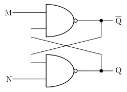
Figure 46: Question 10’s latch: two cross-coupled NAND gates, with M into the top gate (whose output is labelled Q-bar) and N into the bottom gate (whose output is labelled Q).
| M | N | Q | \(\overline{\mathrm{Q}}\) |
|---|---|---|---|
| 0 | 0 | Q | \(\overline{\mathrm{Q}}\) |
| 0 | 1 | 1 | 0 |
| 1 | 0 | 0 | 1 |
| 1 | 1 | 0 | 0 |
| M | N | Q | \(\overline{\mathrm{Q}}\) |
|---|---|---|---|
| 0 | 0 | 1 | 1 |
| 0 | 1 | 0 | 1 |
| 1 | 0 | 1 | 0 |
| 1 | 1 | Q | \(\overline{\mathrm{Q}}\) |
| M | N | Q | \(\overline{\mathrm{Q}}\) |
|---|---|---|---|
| 0 | 0 | 1 | 1 |
| 0 | 1 | 1 | 0 |
| 1 | 0 | 0 | 1 |
| 1 | 1 | Q | \(\overline{\mathrm{Q}}\) |
| M | N | Q | \(\overline{\mathrm{Q}}\) |
|---|---|---|---|
| 0 | 0 | 0 | 0 |
| 0 | 1 | 1 | 0 |
| 1 | 0 | 0 | 1 |
| 1 | 1 | Q | \(\overline{\mathrm{Q}}\) |
- None of the above
TipAnswer
(b)
This is the standard cross-coupled NAND latch, so both inputs are active low. Call the top gate’s output \(P\) (the one the paper labels \(\overline{\mathrm{Q}}\)) and the bottom gate’s output \(Q\). Then
\[P = \overline{M \cdot Q} \qquad Q = \overline{P \cdot N}\]
Work the four input combinations:
- M = 0, N = 0. A 0 on a NAND input forces its output to 1, so both gates output 1: \(Q = 1\) and \(\overline{\mathrm{Q}} = 1\). This is the forbidden combination — the two outputs are not complements.
- M = 0, N = 1. The top gate is forced, \(P = 1\). Then \(Q = \overline{1 \cdot 1} = 0\). So \(Q = 0\), \(\overline{\mathrm{Q}} = 1\) — a clear.
- M = 1, N = 0. The bottom gate is forced, \(Q = 1\). Then \(P = \overline{1 \cdot 1} = 0\). So \(Q = 1\), \(\overline{\mathrm{Q}} = 0\) — a set.
- M = 1, N = 1. Neither gate is forced, so \(P = \overline{Q}\) and \(Q = \overline{P}\), which is satisfied by either stored value. This is the hold state.
That is exactly table (b): \(1,1\) then \(0,1\) then \(1,0\) then hold.
The traps are worth naming. Table (a) puts the hold row at \(00\) and the forbidden row at \(11\) — that is the cross-coupled NOR latch, which has active-high inputs. Tables (c) and (d) get the hold row right but flip the set and clear rows, or write the forbidden state as \(0,0\) instead of \(1,1\) (NANDs cannot both output 0). See flip-flops-and-latches.
Q11 — Which circuit is a latch
Which of the following circuits is capable of acting as a latch? i.e. it has combinations of inputs (M,N) which allow a bit (0 or 1) to be stored, the latch to be set (Q=1) with a single input transition, and the latch to be cleared (Q=0) with a single input transition?
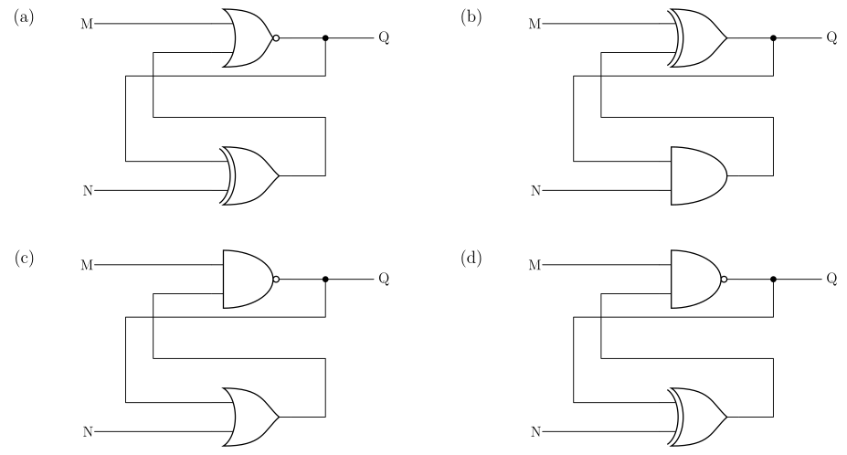
Figure 47: Question 11’s four candidate circuits, wired identically and differing only in the two gate types: (a) NOR over XOR, (b) XOR over AND, (c) NAND over OR, (d) NAND over XOR. In each, M feeds the top gate whose output is Q, N feeds the bottom gate, and the two are cross-coupled.
- None of the above
TipAnswer
(e)
All four circuits are wired the same way. Writing \(P\) for the bottom gate’s output, each is \(Q = g_{\text{top}}(M, P)\) and \(P = g_{\text{bot}}(Q, N)\), so the whole question is which pair of gate types gives a working memory element. For each circuit, substitute both equations into each other for all four \((M,N)\) and see whether the result is consistent (a stable state), forced (set or clear), or self-contradictory (the circuit oscillates).
(a) NOR over XOR — \(Q = \overline{M + P}\), \(P = Q \oplus N\).
| M N | working | result |
|---|---|---|
| 0 0 | \(P = Q\), so \(Q = \overline{Q}\) | oscillates |
| 0 1 | \(P = \overline{Q}\), so \(Q = Q\) | hold |
| 1 0 | \(Q = 0\), \(P = 0\) | clear |
| 1 1 | \(Q = 0\), \(P = 1\) | clear |
From the hold state \(01\), changing M gives \(11\) (a clear) but changing N gives \(00\) (oscillation). It can be cleared but never set.
(b) XOR over AND — \(Q = M \oplus P\), \(P = Q.N\). States: \(00\) clear, \(01\) hold, \(10\) set, \(11\) oscillates. The hold state \(01\) can reach the clear at \(00\) in one transition, but reaching the set at \(10\) needs two. Fails.
(c) NAND over OR — \(Q = \overline{M.P}\), \(P = Q + N\). With \(M = 0\) the NAND is forced, so \(Q = 1\) regardless of N; with \(M = 1, N = 1\) we get \(Q = 0\); with \(M = 1, N = 0\) it oscillates. There is no hold state at all, so this circuit has no memory.
(d) NAND over XOR — \(Q = \overline{M.P}\), \(P = Q \oplus N\). States: \(00\) and \(01\) both set (\(Q = 1\)), \(10\) oscillates, \(11\) holds. From the hold state \(11\), changing M gives a set, but changing N gives oscillation. It can be set but never cleared.
So none of the four does all three jobs, and the answer is (e). This is the point of the question: the classic latches are cross-coupled NOR pairs (hold at \(00\), set and clear on either input alone) or cross-coupled NAND pairs (hold at \(11\), as in Q10), and none of these four mixed pairs reproduces that. See flip-flops-and-latches.
Check this one. All eight gate symbols have now been read twice, independently, at high magnification against the source PDF, and both readings agree with the identifications above. The whole answer still turns on them, though: read the bottom gate of (a) as a NOR rather than an XOR and (a) becomes the textbook NOR latch, making it the answer instead.
Q12 — Timing diagram of a function
Which of the following timing diagrams represents the function \(A.B.C + \overline{B}.C\) ?
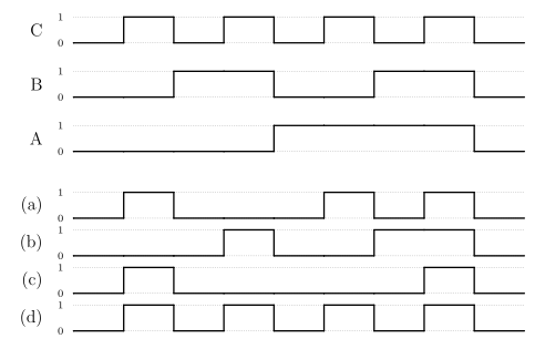
Figure 48: Question 12’s timing diagrams. The top three traces are the inputs C, B and A, which between them count 000 to 111 over the first eight slots and return to 000 in the ninth; the bottom four are the candidate outputs.
- None of the above
TipAnswer
(a)
The three input traces are a binary counter: C toggles every slot, B every two, A every four, so over the nine slots \(A B C\) runs \(000, 001, 010, 011, 100, 101, 110, 111\) and then back to \(000\). That turns the timing diagram into a truth table read left to right.
Evaluating \(F = A.B.C + \overline{B}.C\) slot by slot:
| slot | A B C | \(A.B.C\) | \(\overline{B}.C\) | F |
|---|---|---|---|---|
| 1 | 000 | 0 | 0 | 0 |
| 2 | 001 | 0 | 1 | 1 |
| 3 | 010 | 0 | 0 | 0 |
| 4 | 011 | 0 | 0 | 0 |
| 5 | 100 | 0 | 0 | 0 |
| 6 | 101 | 0 | 1 | 1 |
| 7 | 110 | 0 | 0 | 0 |
| 8 | 111 | 1 | 0 | 1 |
| 9 | 000 | 0 | 0 | 0 |
So the output is high in slots 2, 6 and 8 and low everywhere else, which is trace (a).
The other traces are each a different function of the same inputs: (d) is simply C, which would be the answer if the \(B\) terms were missing; (c) is high only in slots 2 and 8, i.e. it drops the \(101\) case; and (b) is high in slots 4, 7 and 8, which is a different function entirely. See timing-diagrams and logic-gates.
Q13 — Multiplexer as a function
Consider the following multiplexer. What must the inputs A,B,C,D be so that the multiplexer implements the function \(X = S_1 + S_0.G\)?
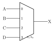
Figure 49: Question 13’s four-to-one multiplexer: inputs A, B, C and D on lines 0 to 3, selected by S1 S0, with output X.
A=0 B=G C=1 D=1
A=1 B=1 C=0 D=G
A=1 B=1 C=G D=0
A=G B=G C=1 D=1
A=G B=0 C=1 D=1
TipAnswer
(a)
A multiplexer whose select lines are the function’s own variables is just a lookup table: input \(n\) is passed through when \(S_1 S_0\) is the binary encoding of \(n\), so input \(n\) must carry whatever the function evaluates to for that combination of selects. Any variable not used as a select — here \(G\) — is allowed to appear on the data inputs.
Evaluating \(X = S_1 + S_0.G\) for each select value:
| \(S_1 S_0\) | line | \(X = S_1 + S_0.G\) | required input |
|---|---|---|---|
| 00 | 0 | \(0 + 0 \cdot G = 0\) | A = 0 |
| 01 | 1 | \(0 + 1 \cdot G = G\) | B = \(G\) |
| 10 | 2 | \(1 + 0 \cdot G = 1\) | C = 1 |
| 11 | 3 | \(1 + 1 \cdot G = 1\) | D = 1 |
So A=0, B=\(G\), C=1, D=1, which is option (a). Note how \(S_1 = 1\) makes the function true whatever \(S_0\) and \(G\) are, which is why both of the bottom two lines are hard-wired to 1. See combinational-logic-blocks.
Q14 — Two’s complement addition
What is the result of adding the 6-bit two’s complement numbers 010110 and 110011?
000001
001001
100101
101001
110111
TipAnswer
(b)
Add the bit patterns as if they were unsigned, then throw away anything past the sixth bit — that is the whole trick of two’s complement, and it is why the same adder works for signed and unsigned:
\[\begin{array}{r} 010110 \\ +\;110011 \\ \hline 1\,001001 \end{array}\]
Column by column from the right: \(0+1 = 1\); \(1+1 = 0\) carry 1; \(1+0+1 = 0\) carry 1; \(0+0+1 = 1\); \(1+1 = 0\) carry 1; \(0+1+1 = 0\) carry 1. Discarding the carry out of the top bit leaves \(001001\).
Sanity check in decimal: \(010110 = 22\), and \(110011\) is negative, with magnitude \(\overline{110011} + 1 = 001100 + 1 = 001101 = 13\), so it is \(-13\). And \(22 - 13 = 9 = 001001\). The result is positive and within range, so the discarded carry is not an overflow. See binary-number-representations.
Q15 — Detecting overflow
Which of the following operations will result in an overflow in 4-bit two’s complement arithmetic?
0100+0101
0100–0101
1001–0001
1001+0001
None of the above
TipAnswer
(a)
Four-bit two’s complement covers \(-8\) to \(+7\). Overflow means the true mathematical result falls outside that range; equivalently, it happens only when the two operands have the same sign and the result has the opposite sign.
| decimal | result | in range? | |
|---|---|---|---|
| (a) \(0100 + 0101\) | \(4 + 5\) | \(9\) | no — overflow |
| (b) \(0100 - 0101\) | \(4 - 5\) | \(-1\) | yes |
| (c) \(1001 - 0001\) | \(-7 - 1\) | \(-8\) | yes, just |
| (d) \(1001 + 0001\) | \(-7 + 1\) | \(-6\) | yes |
Only (a) escapes. Its bit sum is \(0100 + 0101 = 1001\), which reads as \(-7\) — two positives adding to a negative, the classic signature of overflow.
Option (c) is the near miss worth checking carefully: \(-8\) is representable in four bits (it is the one asymmetry of two’s complement), so \(1001 - 0001 = 1000 = -8\) is a legitimate result. Note also that (b) and (d) can never overflow at all, since adding numbers of opposite signs always produces a result no larger in magnitude than the larger operand. See binary-number-representations.
These same four operations also come up in Learning Lab 3 (Binary Arithmetic), in a different order and with the same answer, so this is a question the course drills rather than a one-off. See week2-lab-binary-arithmetic.
Q16 — Interpreting an overflow
Consider the binary addition operation 1001 + 1110. Which of the following statements is true if the numbers are interpreted as two’s complement?
The result is negative and no overflow occurs
The result should be negative but overflow occurs
The result is positive and no overflow occurs
The result should be positive but overflow occurs
The result is zero
TipAnswer
(b)
As two’s complement values, \(1001 = -7\) and \(1110 = -2\), so the true answer is \(-9\) — outside the \(-8\) to \(+7\) range, hence an overflow. The correct answer “should be negative”, which rules out (d).
Doing the addition confirms it:
\[\begin{array}{r} 1001 \\ +\;1110 \\ \hline 1\,0111 \end{array}\]
Discarding the carry leaves \(0111 = +7\): two negatives have produced a positive, which is precisely the overflow signature and is why (a) and (c) are wrong. The carry out of the top bit is not itself the overflow flag here — a two’s complement addition can produce a carry out with no overflow at all (as in Q14). See binary-number-representations.
Q17 — D flip-flop timing
Consider the flip-flop circuit shown below and the associated CLK and output (Q) signals. Which timing diagram shows input (A) values over time which would have resulted in the given output (Q).
Figure 50: Question 17’s positive-edge-triggered D flip-flop, the given CLK and Q traces, and the five candidate A inputs.
TipAnswer
(d)
The clock triangle on the symbol has no bubble, so this is a positive-edge-triggered D flip-flop: at each rising clock edge, Q takes the value D had just before that edge, and between edges Q holds. There are four rising edges in the diagram. Reading the Q trace against them:
| edge | Q before | Q after | so A just before the edge must be |
|---|---|---|---|
| 1 | 0 | 1 | 1 |
| 2 | 1 | 1 | 1 |
| 3 | 1 | 0 | 0 |
| 4 | 0 | 1 | 1 |
So the requirement is \(A = 1, 1, 0, 1\) at the four edges. Checking each candidate:
- (a) goes low right at the first edge and only comes back high at the second, so it reads \(1, 0, \dots\) — wrong at edge 2. (Its transitions also land exactly on the clock edges, which would be a setup-time violation in real hardware.)
- (b) is high at edges 1, 2 and 3, so Q would stay high at edge 3 instead of falling.
- (c) gets edges 1, 2 and 3 right but is low at edge 4, so Q would not rise again.
- (d) is high until part-way through the third clock cycle and low until part-way through the fifth, giving \(1, 1, 0, 1\) — a match, and with every transition comfortably away from a clock edge.
- (e) has already gone low before edge 2, so Q would fall there.
Only (d) works. The useful habit here is to ignore the shape of A between edges entirely: a D flip-flop samples, so only the four instants matter. See flip-flops-and-latches and timing-diagrams.
Q18 — Load-or-swap register pair
Consider the following circuit. If \(A_1\) is 1 and \(A_0\) is 0, what will be the values of \(Q_1\) and \(Q_0\) after three rising clock edges if FN is 0 for one rising clock edge then 1 for two rising clock edges?
Figure 51: Question 18’s circuit: two D flip-flops, each fed by a multiplexer selected by FN. With FN=0 each flip-flop loads its own A input; with FN=1 each loads the other flip-flop’s output, so the pair swaps.
\(Q_1 = 0\) \(Q_0 = 0\)
\(Q_1 = 0\) \(Q_0 = 1\)
\(Q_1 = 1\) \(Q_0 = 0\)
\(Q_1 = 1\) \(Q_0 = 1\)
Insufficient information is provided to determine the values
TipAnswer
(c)
Read the two multiplexers first. Both take their select from FN, so FN picks one of two behaviours for the whole circuit:
- FN = 0 selects line 0 on each multiplexer, which is \(A_1\) for the left flip-flop and \(A_0\) for the right one. This is a parallel load.
- FN = 1 selects line 1. The left multiplexer’s line 1 comes from the long feedback rail running back from \(Q_0\), and the right multiplexer’s line 1 comes from \(Q_1\). So \(D_1 = Q_0\) and \(D_0 = Q_1\) — the two bits swap.
Both flip-flops share the clock, so the swap happens simultaneously and there is no race: each captures the other’s old value.
Now trace the three edges with \(A_1 A_0 = 10\):
| edge | FN | action | \(Q_1 Q_0\) after |
|---|---|---|---|
| 1 | 0 | load \(A_1 A_0\) | 1 0 |
| 2 | 1 | swap | 0 1 |
| 3 | 1 | swap | 1 0 |
After three edges \(Q_1 = 1\) and \(Q_0 = 0\), which is option (c). Two swaps cancel, so the pair is back to what the load put there — which is the real point of the question.
Option (e) is the trap for anyone who worries about the initial contents of the flip-flops, but the first edge loads both of them from \(A_1\) and \(A_0\), so whatever they held beforehand is irrelevant. See sequential-circuits and shift-registers.
Q19 — Flip-flops for a sequence
A sequential circuit has four outputs (\(X_3,X_2,X_1,X_0\)) which advance through the following repeating sequence:
\[X_3X_2X_1X_0: \quad 0000 \to 0001 \to 0011 \to 0111 \to 1111 \to 1100 \to 0000 \to \dots\]
What is the minimum number of flip-flops needed to implement this circuit?
2
3
4
6
8
TipAnswer
(b)
Count the distinct values in the cycle: \(0000\), \(0001\), \(0011\), \(0111\), \(1111\), \(1100\) — six of them, and then it repeats. The flip-flops have to hold the state, not the outputs, and \(n\) flip-flops give \(2^n\) states, so we need the smallest \(n\) with \(2^n \ge 6\):
\[2^2 = 4 < 6 \le 8 = 2^3\]
so three flip-flops, which is (b).
The obvious answer is (c), four — one flip-flop per output bit. That works, and it is what you would build if you wanted the outputs straight off the flip-flops with no extra logic. But the question asks for the minimum, and with only six states in the cycle you can encode the state in three bits and derive the four outputs combinationally from that encoding. The cost is a block of output logic; the saving is a flip-flop.
Note that two would not do: four states cannot distinguish six points in the cycle, and each state must have a unique successor, so distinct steps need distinct encodings. See [counters] and state-machines.
Q20 — Tracing a synchronous counter
What sequence will the following synchronous counter count through, if it starts at \(Q_1Q_0 = 00\)?
Figure 52: Question 20’s counter. The XOR is drawn mirrored, as in the paper: its output faces left into the first flip-flop’s D input and its two inputs face right onto the Q1 and Q0 lines. The NAND takes the same two signals and drives the second flip-flop.
\(Q_1Q_0\): \(00 \to 01 \to 10 \to 11 \to 00 \to \dots\)
\(Q_1Q_0\): \(00 \to 01 \to 11 \to 00 \to \dots\)
\(Q_1Q_0\): \(00 \to 01 \to 11 \to 10 \to 00 \to \dots\)
\(Q_1Q_0\): \(00 \to 10 \to 11 \to 00 \to \dots\)
\(Q_1Q_0\): \(00 \to 11 \to 00 \to \dots\)
TipAnswer
(b)
Both gates see the same two signals — the top rail carries \(Q_0\) back from the second flip-flop, and the vertical line carries \(Q_1\) from the first — so the excitation equations are
\[D_1 = Q_1 \oplus Q_0 \qquad D_0 = \overline{Q_1 \cdot Q_0}\]
Both flip-flops share the clock, so on each edge they update together from the current state. Building the state table:
| \(Q_1Q_0\) | \(D_1 = Q_1 \oplus Q_0\) | \(D_0 = \overline{Q_1.Q_0}\) | next |
|---|---|---|---|
| 00 | 0 | 1 | 01 |
| 01 | 1 | 1 | 11 |
| 11 | 0 | 0 | 00 |
| 10 | 1 | 1 | 11 |
Starting at \(00\) the counter goes \(00 \to 01 \to 11 \to 00\), a three-state cycle, which is option (b).
The fourth row is the unused state. It is worth checking because a counter that can lock up in an unused state is broken: \(10 \to 11\), which is inside the main cycle, so the circuit self-corrects within one clock. See [counters].
Q21 — Counter width
What’s the minimum number of flip-flops needed to build a synchronous binary counter capable of counting from 0 to 16 (inclusive)?
3
4
5
16
17
TipAnswer
(c)
“0 to 16 inclusive” is seventeen values, not sixteen — that is the whole question. With \(n\) flip-flops a binary counter has \(2^n\) distinct states, so we need \(2^n \ge 17\):
\[2^4 = 16 < 17 \le 32 = 2^5\]
so five flip-flops. Four would get to 15 and no further.
Option (b) is what you get by reading “16” as the count of values rather than the last value, and options (d) and (e) confuse flip-flops with states — a one-hot ring counter would need one flip-flop per state, but a binary counter encodes the count in binary, which is exactly why it only needs \(\lceil \log_2 17 \rceil = 5\). See [counters].
Q22 — State diagram to state table
Consider the state diagram below.
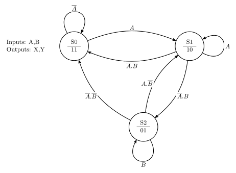
Figure 53: Question 22’s state diagram. Three states, each labelled with its name over its X,Y output pair; every arc carries the condition on the inputs A and B under which it is taken.
Which of the following is an equivalent state table?
| Current State | AB=00 | AB=01 | AB=10 | AB=11 | Outputs (X,Y) |
|---|---|---|---|---|---|
| S0 | S0 | S0 | S1 | S1 | 11 |
| S1 | S0 | S2 | S1 | S2 | 10 |
| S2 | S0 | S2 | S1 | S2 | 01 |
| Current State | AB=00 | AB=01 | AB=10 | AB=11 | Outputs (X,Y) |
|---|---|---|---|---|---|
| S0 | S0 | S1 | S0 | S1 | 11 |
| S1 | S0 | S2 | S1 | S1 | 10 |
| S2 | S0 | S1 | S2 | S2 | 01 |
| Current State | AB=00 | AB=01 | AB=10 | AB=11 | Outputs (X,Y) |
|---|---|---|---|---|---|
| S0 | S0 | S1 | S0 | S1 | 00 |
| S1 | S0 | S2 | S1 | S1 | 01 |
| S2 | S0 | S2 | S1 | S2 | 10 |
| Current State | AB=00 | AB=01 | AB=10 | AB=11 | Outputs (X,Y) |
|---|---|---|---|---|---|
| S0 | S0 | S0 | S1 | S1 | 11 |
| S1 | S0 | S2 | S1 | S1 | 10 |
| S2 | S0 | S2 | S1 | S2 | 01 |
- None of the above
TipAnswer
(d)
Take each state’s outgoing arcs and expand their conditions into the four values of \(AB\). Note that the diagram’s labels do not all name both inputs — \(A\) on its own covers \(AB = 10\) and \(AB = 11\), and \(B\) on its own covers \(01\) and \(11\) — which is where most of the difference between the options lives.
S0 has two arcs: a self-loop on \(\overline{A}\) and an arc to S1 on \(A\). So \(AB = 00, 01 \to\) S0 and \(AB = 10, 11 \to\) S1.
S1 has three arcs: a self-loop on \(A\), an arc to S0 on \(\overline{A}.\overline{B}\), and an arc to S2 on \(\overline{A}.B\). So \(AB = 00 \to\) S0, \(01 \to\) S2, and \(10, 11 \to\) S1 (both covered by the bare \(A\)).
S2 has three arcs: a self-loop on \(B\), an arc to S1 on \(A.\overline{B}\), and an arc to S0 on \(\overline{A}.\overline{B}\). So \(AB = 01, 11 \to\) S2 (both covered by the bare \(B\)), \(10 \to\) S1 and \(00 \to\) S0.
Each state’s arcs cover all four combinations exactly once, which is the completeness check worth doing before comparing anything. The outputs are read straight off the bottom half of each circle: S0 is 11, S1 is 10, S2 is 01.
That gives table (d). The near-miss is (a), which is identical except that it sends S1 to S2 on \(AB = 11\) — that would be right if S1’s self-loop were labelled \(A.\overline{B}\) rather than plain \(A\). Table (b) mangles S0’s row (sending it to S1 on \(01\) instead of \(10\)), and (c) has the outputs shifted onto the wrong states. See state-machines.
The table you have just built is the 2-dimensional state table of the lab’s design pipeline — one row per state, one next-state column per input combination. It is step 2 of six; Beyond the paper below walks the remaining four on a machine of the same size, ending in the waveforms that circuit produces.
Q23 — Tracing a state machine
Consider the state machine represented by the state diagram shown in question 22 (see Q22). What sequence of states is traversed if the machine starts in state S0 and A goes through the sequence 1010101 and B is always the inverse of A?
S0→S0→S1→S2→S1→S2→S1→S2
S0→S1→S1→S2→S1→S2→S1→S2
S0→S1→S2→S2→S1→S2→S1→S2
S0→S1→S2→S1→S2→S1→S2→S1
None of the above
TipAnswer
(d)
B is the inverse of A, so the input pairs alternate between \(AB = 10\) and \(AB = 01\): seven values of A give the sequence \(10, 01, 10, 01, 10, 01, 10\).
From the state table derived in Q22, only two columns are ever used:
- \(AB = 10\): S0 → S1, S1 → S1, S2 → S1
- \(AB = 01\): S0 → S0, S1 → S2, S2 → S2
Starting in S0:
| step | AB | from | to |
|---|---|---|---|
| 1 | 10 | S0 | S1 |
| 2 | 01 | S1 | S2 |
| 3 | 10 | S2 | S1 |
| 4 | 01 | S1 | S2 |
| 5 | 10 | S2 | S1 |
| 6 | 01 | S1 | S2 |
| 7 | 10 | S2 | S1 |
So the machine goes S0→S1→S2→S1→S2→S1→S2→S1, which is (d) — eight states listed, being the start state plus one per input.
The trap is (a), which begins S0→S0 as if the first input left the machine where it was; but the first input has \(A = 1\), and S0 only stays put on \(\overline{A}\). Options (b) and (c) each stutter once in the middle, which cannot happen because the input never repeats. See state-machines. For what a traced machine looks like once it is built out of flip-flops and gates, see Beyond the paper below.
Q24 — ALU control settings
Consider the ALU bit slice below (not the same as seen previously).
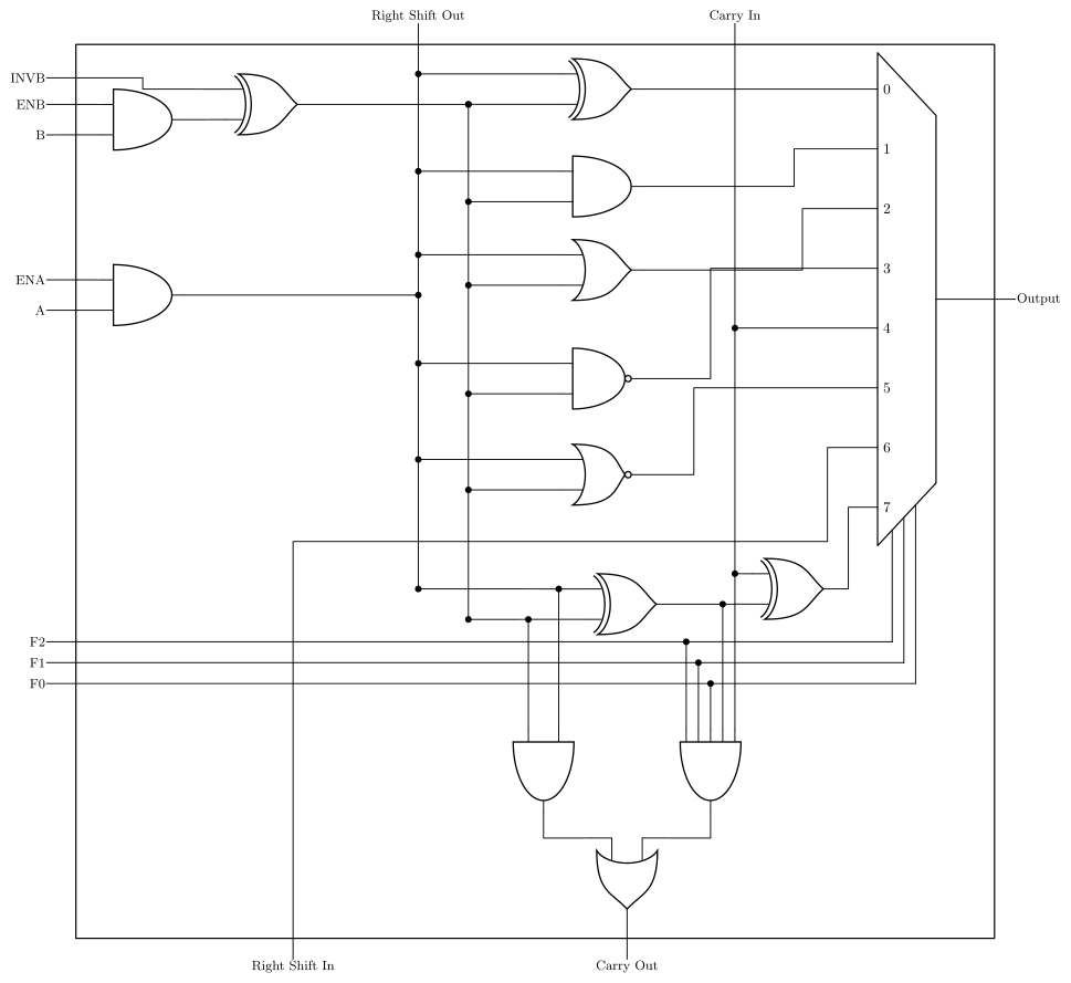
Figure 54: Question 24’s ALU bit slice. ENA/ENB/INVB condition A and B into the internal X and Y rails; five gates and the adder compute their functions in parallel, and the eight-way multiplexer picks one under F2 F1 F0. Right Shift Out is the X rail itself, so selecting input 6 (Right Shift In) hands each slice the bit from the slice to its left.
For an ALU made up of 8 of the bit slices above, which of the following control input settings will result in the ALU output being \(\overline{A}.B\) (bitwise)? (The “Right Shift In” control input refers to that for the most significant bit; the “Carry in” control input refers to that for the least significant bit.)
ENA=1 ENB=1 INVB=0 \(F_2\)=0 \(F_1\)=0 \(F_0\)=0 Right Shift In=1 Carry in=1
ENA=1 ENB=1 INVB=0 \(F_2\)=0 \(F_1\)=0 \(F_0\)=1 Right Shift In=1 Carry in=1
ENA=1 ENB=1 INVB=1 \(F_2\)=0 \(F_1\)=0 \(F_0\)=1 Right Shift In=1 Carry in=1
ENA=1 ENB=1 INVB=0 \(F_2\)=0 \(F_1\)=1 \(F_0\)=1 Right Shift In=1 Carry in=1
ENA=1 ENB=1 INVB=1 \(F_2\)=1 \(F_1\)=0 \(F_0\)=1 Right Shift In=1 Carry in=1
TipAnswer
(e)
Two things have to be read off the figure: what the conditioning gates do to A and B, and which function each value of \(F_2F_1F_0\) selects.
Conditioning. A goes through one AND gate with ENA and nothing else — note there is no INVA on this slice — so the internal signal is
\[X = A \cdot \text{ENA}\]
B goes through an AND with ENB and then an XOR with INVB, and XORing with 1 is inversion, so
\[Y = (B \cdot \text{ENB}) \oplus \text{INVB}\]
Every option sets ENA = ENB = 1, so \(X = A\) and \(Y = B \oplus \text{INVB}\); INVB is the only thing left that can change the data.
Function select. Following each mux input back to its source in the figure gives:
| \(F_2F_1F_0\) | input | function |
|---|---|---|
| 000 | 0 | \(X \oplus Y\) |
| 001 | 1 | \(X \cdot Y\) |
| 010 | 2 | \(X + Y\) |
| 011 | 3 | \(\overline{X \cdot Y}\) |
| 100 | 4 | Carry In |
| 101 | 5 | \(\overline{X + Y}\) |
| 110 | 6 | Right Shift In |
| 111 | 7 | \(X \oplus Y \oplus C_{in}\) (the sum) |
Now, how do you get \(\overline{A}.B\) from a slice that cannot invert A? Push the complement onto the other side with De Morgan:
\[\overline{A}.B = \overline{A + \overline{B}}\]
So take \(X = A\) and \(Y = \overline{B}\) (which needs INVB = 1) and select the NOR, which is \(F_2F_1F_0 = 101\). That is option (e).
Checking the others: (a) is INVB = 0 with the XOR, giving \(A \oplus B\); (b) is INVB = 0 with the AND, giving \(A.B\); (c) is INVB = 1 with the AND, giving \(A.\overline{B}\) — the mirror image of what was asked, and the most tempting wrong answer; (d) is INVB = 0 with the NAND (\(F_2F_1F_0 = 011\)), giving \(\overline{A.B}\), which is the complement of (b) rather than anything with a single complemented variable.
Right Shift In and Carry in are set to 1 in every option, so they cannot distinguish the answers — and neither reaches the output anyway once \(F_2F_1F_0\) selects a logic function. See arithmetic-logic-unit.
Q25 — What the ALU cannot do
For an ALU made up of 8 of the bit slices shown in question 24 above (see Q24), which of the following control input function settings can NOT be used to output \(\overline{B}\) (bitwise) — assuming other control inputs are chosen appropriately?
\(F_2\)=0 \(F_1\)=0 \(F_0\)=0 XOR
\(F_2\)=0 \(F_1\)=1 \(F_0\)=0 OR
\(F_2\)=0 \(F_1\)=1 \(F_0\)=1 NAND
\(F_2\)=1 \(F_1\)=0 \(F_0\)=1 NOR
None of the above
TipAnswer
(c)
The question hands you the function each select code picks, so the work is in what the conditioning gates can produce. From Q24, the two internal signals are \(X = A \cdot \text{ENA}\) and \(Y = (B \cdot \text{ENB}) \oplus \text{INVB}\), so the reachable values are:
| ENA | \(X\) | ENB | INVB | \(Y\) | |
|---|---|---|---|---|---|
| 0 | \(0\) | 0 | 0 | \(0\) | |
| 1 | \(A\) | 0 | 1 | \(1\) | |
| 1 | 0 | \(B\) | |||
| 1 | 1 | \(\overline{B}\) |
The critical asymmetry is that X can be forced to 0 but never to 1, because there is no INVA on this slice. Y, having the INVB stage, can be forced to either constant.
With that in hand:
- (a) XOR, \(X \oplus Y\). Set ENA = 0 so \(X = 0\), and ENB = INVB = 1 so \(Y = \overline{B}\). Then \(0 \oplus \overline{B} = \overline{B}\), so this one works.
- (b) OR, \(X + Y\). Same settings: \(0 + \overline{B} = \overline{B}\), so this one works too.
- (d) NOR, \(\overline{X + Y}\). Set \(X = 0\) and \(Y = B\) (ENB = 1, INVB = 0). Then \(\overline{0 + B} = \overline{B}\), which works.
- (c) NAND, \(\overline{X \cdot Y}\). To get \(\overline{B}\) out of a NAND you need \(X \cdot Y = B\), which requires \(X = 1\) with \(Y = B\) (or \(X = B\), which is not available either — A and B cannot be swapped). But \(X \in \{0, A\}\), so \(X\) can never be a constant 1. Every reachable combination fails: \(X = 0\) gives a constant 1; \(X = A\) gives \(\overline{A.B}\), \(\overline{A.\overline{B}}\), \(\overline{A}\) or 1, none of which is \(\overline{B}\). This is the one that cannot be done.
So (c) is the setting that cannot produce \(\overline{B}\). The general lesson is the one from arithmetic-logic-unit: forcing a data input to a constant is what lets one ALU compute unary functions, and here that trick works on the B side but only half-works on the A side.
Beyond the paper — from state diagram to wired circuit
Q22 asks for one step of a longer road — state diagram to state table — and Q23 asks you to walk the machine along it. Learning Lab 8 (State Machines) names the whole road and makes you travel all of it: “do hand design first — state diagram → state table → next state logic and output logic”, and then “enter the circuit into Logisim and simulate it”.
This follows the design task of Learning Lab 8 (State Machines). Its Design Task 1, a detector for the sequence
001, is worked through state diagram, state tables, encoding, Boolean expressions and logic diagram in week5-lab-state-machines. This section maps the lab’s design steps onto this paper’s questions and adds a timing diagram of the finished design, using the encoding and expressions from that note.
The pipeline, and where this paper cuts into it
| Step | What Lab 8 asks for | Tested here by |
|---|---|---|
| 1 | Draw the state diagram — one circle per state, name over output, an arrow per input condition | Q22 reads one; Q23 walks one |
| 2 | Write the 2-dimensional state table — one row per state, one next-state column per input combination | Q22, which is exactly this conversion |
| 3 | Choose a state encoding — the number of flip-flops and their values in each state. “Examine different options for state encoding!” | Q19, Q21 — both are the “how many flip-flops” half of this step |
| 4 | Write the 1-dimensional state table — one row per (state, input) combination, with the D inputs spelled out | not examined directly; it is the working for step 5 |
| 5 | Derive Boolean expressions for the outputs and the flip-flop D inputs, in terms of the Q outputs and the inputs | Q20 runs this backwards, reading a counter’s next-state logic off its circuit |
| 6 | Enter the circuit and simulate | the timing diagram below is what that simulation shows |
Step 3 is the one the lab shouts about, and it is worth seeing why. For the 001 detector, the obvious binary assignment \(S_0S_1S_2S_3 = 00,01,10,11\) leaves several product terms in each next-state expression and nothing collapses; the assignment week5-lab-state-machines settles on instead —
\[S_0 = 01 \qquad S_1 = 00 \qquad S_2 = 10 \qquad S_3 = 11\]
— makes one flip-flop input collapse to a bare wire. Nothing about the state diagram changed; only the numbers written on the states did.
What the machine does on a clock
\[D_0 = S \qquad D_1 = \overline{Q_0}\,(Q_1 + \overline{S}) = \overline{Q_0} \cdot \overline{\overline{Q_1}\,.\,S} \qquad X = Q_1 . Q_0\]
Three chips build that: a 74HCT74 for the two flip-flops, one NAND of a 74HCT00, and two ANDs of a 74HCT08 — which is the lab’s “are you a bad enough dude to implement a sequence detector with just three chips?” challenge, answered. The logic diagram is drawn in week5-lab-state-machines; what is worth adding here is the other view of the same machine, because it is the one Q23 and Q17 are really asking about — where each value sits in time.
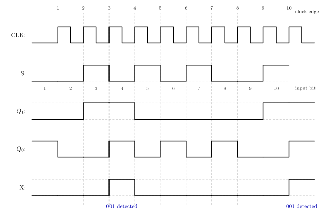
Figure 55: The 001 detector running on the first ten bits of the input sequence from Lab 8’s Design Task 1. Read it in columns: the dashed verticals are the ten rising clock edges, the number under the S track is which input bit is being presented, and each of Q1, Q0 and X holds the value it took at the previous edge. The offset is the whole point. Bit 3 completes the first 001 while it sits in the interval before edge 3, but X only goes high after edge 3 has been taken, so the pulse on X appears one column to the right of the bit that caused it - even though the lab’s S and X strings are written aligned by index. Q0 is a delayed copy of S, which is what D0 = S means in the time domain, and X is high exactly where Q1 and Q0 are both high. The two blue notes are added here, not on the slide.
Three things come off that picture, and each is an exam trap somewhere:
- The input is sampled, not watched. Nothing happens to \(Q_1\) or \(Q_0\) between edges, however \(S\) wriggles. This is the whole content of Q17, where the question is which candidate \(A\) waveform could have produced the given \(Q\) — and the answer only ever depends on what \(A\) was doing at the edges.
- A Moore output lags the input that caused it. Bit 3 completes the first
001, but the machine is only in \(S_3\) after edge 3 has happened, so \(X\) rises after that edge and stays up for one clock period. The lab’s two bit strings are aligned by index, not by time. - \(Q_0\) is \(S\) delayed by one clock, which is exactly what \(D_0 = S\) means once the flip-flop is in the path. Encoding choices that make a D input equal an existing signal turn a gate into a wire, and that is why step 3 of the pipeline is worth the effort.
Two more questions the same design answers
- “How many flip-flops does this machine need?” — Q19 and Q21. Count the states, then count the flip-flops: \(N\) flip-flops hold \(2^N\) distinct patterns, so \(N = \lceil \log_2(\text{number of states}) \rceil\). Four states here, hence the two tracks \(Q_1\) and \(Q_0\) in the waveform.
- “Moore or Mealy?” — \(X = Q_1 . Q_0\) mentions the state and nothing else, which is what makes this Moore. A Mealy output would have \(S\) in its expression too, and would then be free to change part-way through a clock period rather than only just after an edge — the flat-topped one-period-wide pulses on the \(X\) track are the visible signature of Moore. CSSE2010 sticks to Moore; see state-machines.
Your score
Reload the page to clear your answers.
Device Pinouts
Pin numbers for the 74-series logic chips and IO board used in circuit-schematics. All quad 2-input gate chips (74HCT00, 08, 32, 86) share the same pin layout — only the gate function differs.
Source: CSSE2010/CSSE7201 Device Pinouts and Symbols (Blackboard, v4). This is the whole parts list: every gate chip in it is 2-input (plus the hex inverter), so a design needing a 3-or-more-input gate has to be built up from 2-input ones. There is no 3-input AND/OR/NAND in the kit.
The source sheet gives up to three things per device, and they are not interchangeable:
| Column | What it is | Where it is used |
|---|---|---|
| Device pinout | the physical package: which signal is on which numbered pin | wiring the breadboard; checking a schematic’s pin numbers |
| Logic diagram symbol | the hardware-independent shape | logic-gates and logic diagrams |
| Circuit schematic symbol | the shape plus device ID, device type and pin numbers | circuit-schematics |
Power and ground
Power and ground connections for devices are shown separately from the gate pins on a schematic, once per device type. The symbols below are also what you use to tie a device input directly to logic low or logic high.
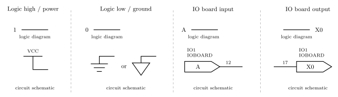
Figure 56: The four non-gate symbols. Logic high and logic low are a bare 1 or 0 on a logic diagram, and a VCC bar or a ground symbol (either of the two accepted forms) on a circuit schematic. The IO board input and output symbols are the same pentagon; the difference is that an input’s wire leaves the point and an output’s wire arrives at the flat back.
Quad 2-input gates (74HCT00 / 08 / 32 / 86)
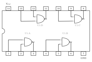
Figure 57: The 14-pin DIP pinout, drawn for the 74HCT00 but identical for the 08, 32 and 86 — only the gate shape inside changes. The notch marks the pin-1 end; pins run 1-7 along the bottom and 14-8 along the top. Reading the internal wiring is what tells you the gates pair pins 1,2 to 3, 4,5 to 6, 9,10 to 8 and 12,13 to 11, and that Vcc (14) and GND (7) are the two pins with no gate on them.
| Chip | Function | Gate A | Gate B | Gate C | Gate D | VCC | GND |
|---|---|---|---|---|---|---|---|
| 74HCT00 | Quad 2-input NAND | in 1,2 → out 3 | in 4,5 → out 6 | in 9,10 → out 8 | in 12,13 → out 11 | 14 | 7 |
| 74HCT08 | Quad 2-input AND | in 1,2 → out 3 | in 4,5 → out 6 | in 9,10 → out 8 | in 12,13 → out 11 | 14 | 7 |
| 74HCT32 | Quad 2-input OR | in 1,2 → out 3 | in 4,5 → out 6 | in 9,10 → out 8 | in 12,13 → out 11 | 14 | 7 |
| 74HCT86 | Quad 2-input XOR | in 1,2 → out 3 | in 4,5 → out 6 | in 9,10 → out 8 | in 12,13 → out 11 | 14 | 7 |
The letters A–D are yours to assign — the chip does not label its own gates. What is fixed is which pins belong to the same gate. Whichever slot you call U1:A, its pin numbers must be one of the four sets above.
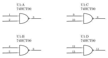
Figure 58: The four gates of a 74HCT00 as circuit schematic symbols: device ID, device type, and a pin number on every terminal. For a 74HCT08, 74HCT32 or 74HCT86 the pin numbers are exactly these; only the gate body changes to AND, OR or XOR.
74HCT04 — Hex inverter
Six independent NOT gates. VCC = pin 14, GND = pin 7.
| Gate | A | B | C | D | E | F |
|---|---|---|---|---|---|---|
| in → out | 1→2 | 3→4 | 5→6 | 9→8 | 11→10 | 13→12 |
Figure 59: All six inverters of a 74HCT04. The numbering is not a simple run: the first three gates go low-to-high (1 to 2, 3 to 4, 5 to 6) but the last three run the other way (9 to 8, 11 to 10, 13 to 12), because the package is symmetric about its centre.
Note the direction reversal in the second half of the package — U1:D is pin 9 in, 8 out, not 8 in, 9 out. Getting this backwards is an easy way to lose marks on a schematic.
74HCT74 — Dual D-type flip-flop (14-pin)
| Pin | 1 | 2 | 3 | 4 | 5 | 6 | 7 | 8 | 9 | 10 | 11 | 12 | 13 | 14 |
|---|---|---|---|---|---|---|---|---|---|---|---|---|---|---|
| Signal | CLR1 | D1 | CLK1 | SET1 | Q1 | \(\overline{Q1}\) | GND | \(\overline{Q2}\) | Q2 | SET2 | CLK2 | D2 | CLR2 | VCC |
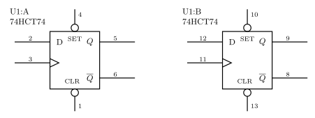
Figure 60: The two flip-flops of a 74HCT74 as circuit schematic symbols. Unlike the 74HCT175 below, each flip-flop has its own clock, its own set and its own clear — nothing is shared. SET and CLR carry bubbles, and the wedge on the left-hand lower input marks the clock.
Set and clear inputs can be omitted from the schematic if not needed — the source sheet says so explicitly, and its own logic-diagram symbol is drawn without them.
74HCT157 — Quad 2-input multiplexer (16-pin)
| Pin | 1 | 2 | 3 | 4 | 5 | 6 | 7 | 8 | 9 | 10 | 11 | 12 | 13 | 14 | 15 | 16 |
|---|---|---|---|---|---|---|---|---|---|---|---|---|---|---|---|---|
| Signal | SEL | A0 | B0 | Y0 | A1 | B1 | Y1 | GND | Y2 | B2 | A2 | Y3 | B3 | A3 | \(\overline{\text{ENABLE}}\) | VCC |
Figure 61: The 74HCT157 as one circuit schematic symbol — the multiplexer trapezoid, tall edge for the eight data inputs and short edge for the four outputs. It is four 2-to-1 multiplexers sharing a single SEL line and a single active-low ENABLE, so it selects between two whole 4-bit words rather than between two individual bits: one value of SEL puts A0-A3 on Y0-Y3 and the other puts B0-B3 there.
SEL (pin 1) and ENABLE (pin 15) are common to all four multiplexers — one select line for the whole package. That is what makes this chip a 4-bit-wide 2-to-1 mux rather than four independent ones. ENABLE is active low — the source sheet writes it \(\overline{\text{ENABLE}}\) and draws a bubble on that pin.
At the logic-diagram level the source sheet allows several options: one wide block with A, B, Y buses and slashes marking the 4-bit widths, or four separate 2-to-1 mux symbols drawn side by side, with the enable input added only if it is needed. See combinational-logic-blocks for what a multiplexer does.
74HCT175 — Quad D-type flip-flop (16-pin)
| Pin | 1 | 2 | 3 | 4 | 5 | 6 | 7 | 8 | 9 | 10 | 11 | 12 | 13 | 14 | 15 | 16 |
|---|---|---|---|---|---|---|---|---|---|---|---|---|---|---|---|---|
| Signal | \(\overline{\text{CLR}}\) | Q0 | \(\overline{Q0}\) | D0 | D1 | \(\overline{Q1}\) | Q1 | GND | CLK | Q2 | \(\overline{Q2}\) | D2 | D3 | \(\overline{Q3}\) | Q3 | VCC |
The ordering is not uniform — check it before wiring. The package is mirror-symmetric about each D-pair, so the true outputs sit at pins 2, 7, 10, 15 and the complements at 3, 6, 11, 14. Reading “Q then \(\overline{Q}\)” left-to-right across all four flip-flops gets flip-flops 1 and 3 backwards. The source’s own schematic symbol settles it: D1 (pin 5) → Q1 (pin 7), D3 (pin 13) → Q3 (pin 15).
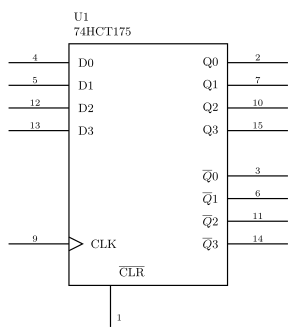
Figure 62: The 74HCT175 as one circuit schematic symbol. CLK (pin 9) and CLR (pin 1) enter once and serve all four flip-flops, which is exactly what a flat pin table hides: this is a 4-bit register, not four independent flip-flops.
CLK (pin 9) and CLR (pin 1) are common to all four flip-flops — one clock and one clear for the whole package. The source sheet’s logic-diagram column shows this two ways: as a single D flip-flop with 4-bit-wide D and Q buses, or as four separate flip-flops whose clock inputs are all tied together.
74HCT283 — 4-bit full adder (16-pin)
| Pin | 1 | 2 | 3 | 4 | 5 | 6 | 7 | 8 | 9 | 10 | 11 | 12 | 13 | 14 | 15 | 16 |
|---|---|---|---|---|---|---|---|---|---|---|---|---|---|---|---|---|
| Signal | S1 | B1 | A1 | S0 | A0 | B0 | C0 | GND | C4 | S3 | B3 | A3 | S2 | A2 | B2 | VCC |
\(C0\) is the carry-in, \(C4\) the carry-out; \(A_i, B_i\) are the two 4-bit operands and \(S_i\) the 4-bit sum.
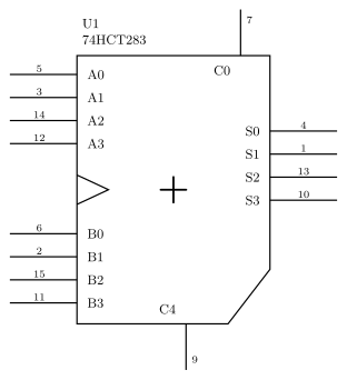
Figure 63: The 74HCT283 as one circuit schematic symbol. Internally it is four full adders with C1, C2 and C3 wired stage to stage inside the package, so only C0 and C4 are brought out to pins.
The source sheet’s logic-diagram column shows the internals as four cascaded full adders, with the intermediate carries \(C_1\), \(C_2\), \(C_3\) entirely inside the chip. It also offers a compact alternative symbol with \(A\), \(B\) and \(S\) drawn as 4-bit buses. This chip is the adder half of the adder-subtractor in combinational-logic-blocks.
IO board
| Pins | Function |
|---|---|
| 1 | TX |
| 2 | RX |
| 3 | SSD cathode |
| 4 | SSD decimal point |
| 5–11 | SSD segments G to A |
| 12–15 | Buttons B3 to B0 |
| 16 | Logic probe |
| 17–24 | LEDs L0 to L7 |
| 25–32 | Switches S0 to S7 |
On a schematic the IO board is labelled IO1 (IO2 for a second board), with inputs using the point-attached symbol and outputs the back-attached symbol — see Figure 56 and circuit-schematics. Use sensible signal names rather than the raw pin labels where possible: the source sheet’s own example names buttons B3–B0 on pins 12–15, switches A–H on pins 25–32, and LED outputs X0–X5, COUT, OFLOW on pins 17–24. There is no need to show power supply connections for the IO board.
Buttons and switches are inputs to your circuit; LEDs and the seven-segment display are outputs. See io-board for what the board does electrically.
Fetch-Decode-Execute Cycle
What the control unit actually does: a continuous cycle over the datapath, issuing control signals in the right order for whatever instruction it just read. See cpu-organisation for the blocks involved and arithmetic-logic-unit for the one being driven.
The cycle
The control unit operates in a continuous cycle on the datapath:
| Stage | What happens |
|---|---|
| Fetch | Fetch an instruction from memory and bring it inside the CPU. Two special purpose registers involved — PC and IR |
| Decode | Resolve the operation (opcode) and operands (variables) |
| Execute | Control signals are issued and the operation takes place in the datapath |
Stated as steps:
- Fetch the next instruction from memory into the Instruction Register (IR).
- Change the Program Counter (PC) to point to the next instruction.
- Determine the type of (decode) the instruction just fetched — i.e. look at the opcode.
- Execute the instruction.
- Return to step 1.
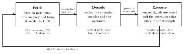
Figure 64: The cycle as a loop: a three-stage pipeline. Each box holds a one-line description of its stage, each arrow carries what the stage leaves behind for the next one, and the notes under the boxes summarise steps 1–4 above.
Step 2 advances the PC before the instruction executes, which is why a jump instruction works by overwriting the PC rather than by suppressing the increment.
The datapath
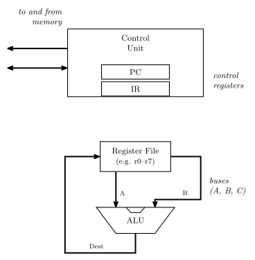
Figure 65: The datapath the cycle runs on. The control unit holds PC and IR and talks to memory; below it, the register file puts two values onto the A and B buses, the ALU combines them, and the result returns on the destination bus to be written back into a register.
The question this raises — and the one the control unit exists to answer — is how do we control this? Specifically:
- How do we tell the ALU what to do?
- How do we choose what register values are placed on the A and B buses?
- How do we choose which register receives the result from the destination bus?
- How do we know when to read or write memory?
Control signals
Each of those questions is answered by a bundle of wires out of the control unit. For a machine with 8 registers and the ALU of arithmetic-logic-unit:
| Signal | Width | Answers |
|---|---|---|
| A register select | 3 | which register drives the A bus (\(2^3 = 8\) registers) |
| B register select | 3 | which register drives the B bus |
| Destination select | 3 | which register the result is written back into |
| ALU control | 6 | what the ALU does — \(F_1\), \(F_0\), ENA, INVA, ENB, INC |
| Memory read/write | 1 | whether this is a read or a write |
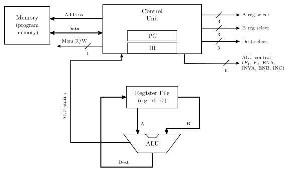
Figure 66: The same datapath with every control signal named. Added to the previous figure: the memory block, the Address, Data and Mem R/W labels, the five bundles with their widths, and the ALU status path back into the control unit. The bundles are drawn as labelled stubs: A/B/Dest select drive the register file, ALU control drives the ALU. Widths are marked with a slash and a number; the course also letters the width beside a plain arrow, and neither is fixed as the standard. Everything except the memory block sits inside the CPU.
Plus the address and data connections to memory itself. The widths are not arbitrary: three bits because there are eight registers, and six bits because the ALU has exactly six control inputs.
Control signals come from the control unit, which must generate them in the right order for a given instruction — and which instruction that is, is determined by the contents of the Instruction Register.
So a line of high-level code like r5 = r0 + r2 becomes: A select = 0, B select = 2, destination select = 5, ALU control = the \(A + B\) row of the combinations table, memory read/write idle.
Data influencing control
The IR is not enough. The control unit can’t operate without knowing something about the data — for example, if a for-loop variable is supposed to count from 10 down to 0, how does the control unit know when it gets there?
The answer is the status register: determined by ALU operations, it stores the status of the last ALU operation and is available to the control unit. This closes the loop — the ALU’s results feed back into the control unit and change what it does next, which is what makes conditional branching possible at all. It is the return path drawn in Figure 66, and it is what a source-level if (x < 0) compiles down to.
ALU status flags
The ALU emits, alongside its result, a summary of what happened during the last operation. Typically stored in a special purpose register called the STATUS register:
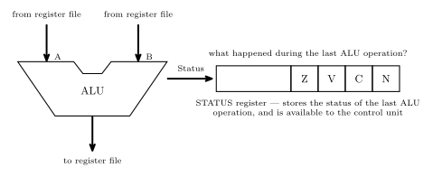
Figure 67: The ALU’s second output. The result goes back to the register file; alongside it the ALU reports what happened, and those flags land in the STATUS register where the control unit can read them. The ALU is drawn as a notched trapezoid here; the block diagram in the ALU note draws the same block as a plain rectangle, and the course uses both shapes. The register is drawn as four named cells at the right-hand end of a wider register. That is shorthand, not a bit-position claim — the AVR’s own SREG orders and numbers its bits differently, see the AVR architecture note.
| Flag | Name | Asks |
|---|---|---|
| Z | zero | was the last result 0? |
| V | overflow | did the last addition/subtraction overflow, assuming it was a two’s complement operation? |
| C | carry | was a carry out generated? |
| N | negative | was the result negative if considered as two’s complement — i.e. what is the sign bit? |
V and N both presuppose a two’s complement interpretation while C does not — the hardware computes all four regardless, and it is the program’s business to read the ones that mean something for the operation it just did. See binary-number-representations, and 2026-08-04-binary-arithmetic for the overflow rules V implements.
Worked example
What values are in the status register flags after the operation \(8_{10} - 9_{10}\) on a 5-bit ALU?
First, \(-9\) in 5-bit two’s complement: \(9 = 01001\), invert to \(10110\), add one to get \(10111\). Then add, tracking the carry into and out of the sign column:
\[\begin{array}{crl} \text{carry into MSB} \rightarrow & 0\phantom{0000} & \\ & 01000 & \\ + & 10111 & \\ \hline \text{carry out} = 0 \rightarrow & 11111 & \end{array}\]
The result is \(11111\), with no carry out of the top bit. So:
| Flag | Value | Why |
|---|---|---|
| Z | 0 | the result \(11111\) is not zero |
| C | 0 | no carry out of the most significant bit |
| V | 0 | the carry into the sign column and the carry out of it agree, both 0 — and indeed \(8 + (-9) = -1\) is comfortably in range for 5-bit two’s complement |
| N | 1 | the sign bit is 1 — the result is negative |
And indeed \(11111\) read as two’s complement is \(-1\), which is \(8 - 9\).
See also
- cpu-organisation · arithmetic-logic-unit
- binary-number-representations — two’s complement, overflow and the sign bit
- 2026-08-04-binary-arithmetic — the \(C_{in} \oplus C_{out}\) overflow test the V flag implements
- avr-architecture — the AVR’s own status register, bit by bit
- state-machines — the control unit is itself a state machine, sequencing signals for each instruction
- 2026-08-24-alu-and-control-unit — Lecture 9
Flip-Flops and Latches
Flip-flops and latches are the storage elements — the circuits that let a design remember a value even after the input that produced it has changed. They’re what turns a combinational circuit into a sequential circuit.
Introduced in Lecture 5, 2026-08-10-introduction-to-sequential-circuits.
The D flip-flop
The D flip-flop is the only flip-flop type covered in this course. Its symbol is a rectangle with:
- D — the data input, on the left.
- Q — the output, on the right.
- CLK — the clock, a control input on the left, drawn with a small triangular wedge where it meets the box.
How it works: Q copies the value of D (and remembers it) whenever CLK goes from 0 to 1 — the rising edge. In between clock edges the flip-flop is not responsive, so it holds the stored value. Q changes only on that 0→1 transition.
Summary: a D flip-flop remembers a single bit — either a “1” or a “0”. It keeps that value until the next clock edge, at which point the D input is transferred to output Q.
- To remember \(n\) bits you need \(n\) D flip-flops.
- An \(n\)-bit register is (by definition) \(n\) D flip-flops. See shift-registers.
- Flip-flops can themselves be made out of logic gates — see the SR latch and A real D flip-flop below.
Characteristic table
A characteristic table defines the operation of a flip-flop in tabular form. The left column is the input; the right column, \(Q(t+1)\), is the next value of Q: what the output will be on the next clock edge (i.e. when CLK goes 0→1).
| D | Q(t+1) | |
|---|---|---|
| 0 | 0 | Reset |
| 1 | 1 | Set |
That is the whole behaviour: the flip-flop is reset (to 0) or set (to 1) according to D, at the clock edge.
A flip-flop’s next-state column is written \(Q(t+1)\) here. The state tables of state-machines and [counters] call the same thing Next State. The course uses both names (see csse2010-diagram-notation).
Worked waveform
D is 0, 0, then 1, 1 across a clock with two rising edges. CLK starts low, pulses high, goes low, then pulses high again after D has risen.
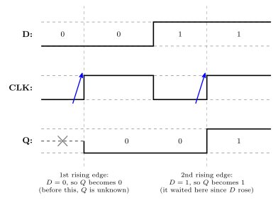
Figure 68: A D flip-flop waveform. The dashed verticals are the two rising clock edges, and the arrows mark them. Q is undefined (drawn dashed, with a cross) until the first edge. The point of the figure is the middle: D rises well before the second edge, and Q does not follow until that edge arrives.
| Clock edge | D at that edge | Q after |
|---|---|---|
| (before the first edge) | — | unknown/undefined |
| 1st rising edge | 0 | 0 |
| 2nd rising edge | 1 | 1 |
Before the first rising edge Q is undefined, because nothing has been clocked in yet; an “X” marks that stretch. Between the two rising edges Q stays 0 even though D has already risen to 1: the flip-flop is only sensitive at the edge. Remember: Q changes only when the clock (CLK) goes from 0 to 1.
A second, harder worked waveform — four clock edges, with D both rising and falling between them — is in 2026-08-10-introduction-to-sequential-circuits.
Other flip-flop types
Other types exist — JK flip-flops and T flip-flops — but they are not covered in this course. Only the D flip-flop is used.
Latches vs flip-flops
- Latches are level triggered devices — they latch the output and respond to changes of logic levels on the inputs.
- A latch circuit can be modified so that it becomes sensitive to an edge (a momentary transition) of a control input, i.e. a clock signal. Such circuits are called flip-flops.
- A flip-flop can store 1 bit of information while being sensitive to a clock edge — it changes its output only at the clock edges, based on the inputs.
- So: latches are level triggered; flip-flops are edge triggered.
A clock signal has two edges:
| Edge | Transition |
|---|---|
| Positive (rising) edge | 0 → 1 |
| Negative (falling) edge | 1 → 0 |
A D flip-flop can therefore be positive edge triggered or negative edge triggered. In a positive edge triggered D flip-flop, D is copied to Q at the positive edge of the clock; in between clock edges the flip-flop is not responsive, thus stores the value.
The state of a flip-flop is the value it is storing. Flip-flops are more useful than latches in practice.
Symbols used
Four related symbols, all drawn as a rectangle with D in at the top left, Q out at the top right, and a clock input CK at the bottom left. What distinguishes them is the marking on that CK input.
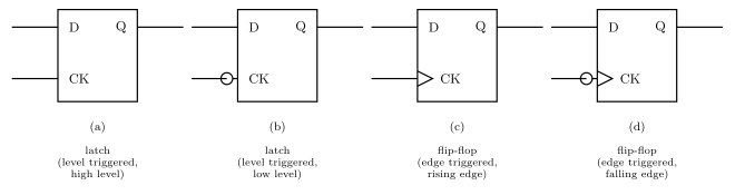
Figure 69: The four latch and flip-flop symbols, with the clock pin labelled CK (the course writes this pin CLK elsewhere). The wedge and the bubble read independently: the wedge says edge-triggered, therefore flip-flop; the bubble says inverted, therefore falling edge or low level. The reading under each symbol follows from those two rules.
| Symbol | CK input marking | Device | Triggered on |
|---|---|---|---|
| (a) | plain input | Latch | High level of CK |
| (b) | bubble (inversion circle) | Latch | Low level of CK |
| (c) | triangle/wedge | Flip-flop | Rising (positive) edge of the clock |
| (d) | bubble + triangle | Flip-flop | Falling (negative) edge of the clock |
The two markings read independently and are the whole key to the notation:
- The triangle indicates edge-triggered, and therefore that the device is a flip-flop rather than a latch. No triangle means level-triggered, i.e. a latch.
- The bubble indicates inversion, i.e. the falling edge (or the low level) rather than the rising edge (or the high level).
The SR latch (cross-coupled NOR gates)
Structure: two 2-input NOR gates cross-coupled.
- The top NOR gate takes \(S\) as one input and the bottom gate’s output as its other input; its output is \(\bar Q\).
- The bottom NOR gate takes \(R\) as one input and the top gate’s output (\(\bar Q\)) as its other input; its output is \(Q\).
So each gate’s output feeds back into the other gate’s input — that feedback loop is what stores the bit.
Figure 70: The SR latch: two cross-coupled NOR gates, with the NOR truth table to remember and the two special cases the analysis needs. Between them they are the whole analysis: a NOR with a 0 on one input passes the other input inverted, and a NOR with a 1 on one input is pinned to 0. Where the two feedback wires cross there is no junction dot, so it is two wires passing, not a connection.
The analysis needs both identities in the figure. Together they are what makes each row fall out in a line. Both are just De Morgan applied to a NOR (see boolean-algebra): \(\overline{A+B} = \bar A \cdot \bar B\).
The truth table:
| S | R | Q | \(\bar Q\) | Meaning |
|---|---|---|---|---|
| 0 | 0 | \(Q_{n-1}\) | — | Storage / remember |
| 0 | 1 | 0 | 1 | Reset |
| 1 | 0 | 1 | 0 | Set |
| 1 | 1 | — | — | Invalid \(\times\) |
\(Q_{n-1}\) means “whatever \(Q\) was before” — the hold row’s entry is not a bit but a reference to the previous value. Three cells are left blank: \(\bar Q\) in the hold row, and both outputs in the last row, which is Invalid.
Reasoning for each row, using the two identities above:
- \(S=0, R=0\): each gate has a 0 on its external input, so each is an inverter of the other’s output — \(\bar Q = \overline{Q}\) and \(Q = \overline{\bar Q}\). Both \(Q=1\) and \(Q=0\) satisfy that, so the latch simply holds whatever it already had. This row is the whole point of the circuit: it is the row in which the latch remembers.
- \(S=1, R=0\): the top gate has a 1 on an input, so \(\bar Q = 0\) regardless. The bottom gate then sees \(R=0\) and \(\bar Q=0\), so \(Q=1\). \(S\) sets the latch.
- \(S=0, R=1\): mirror image — the bottom gate has a 1 on an input, so \(Q=0\); the top gate then sees \(S=0\) and \(Q=0\), so \(\bar Q=1\). \(R\) resets the latch.
- \(S=1, R=1\): both gates have a 1 on an input, so both outputs are 0: \(Q = 0\) and \(\bar Q = 0\). That result is what condemns the combination: the two outputs are supposed to be complements and here they are equal, so the labels \(Q\) and \(\bar Q\) stop meaning anything. Worse, what happens after both inputs return to 0 simultaneously is not uniquely determined (the two gates race), so the resulting state is indeterminate. Hence invalid — a combination you must not apply.
This circuit is the active high SR latch: the inputs do their job when driven to 1, and the resting/hold condition is \(S=R=0\). That name is what distinguishes it from the NAND version below.
The SR latch from NAND gates (active low)
Exercise: analyse the SR latch circuit when the NOR gates are replaced with NAND gates, and complete the truth table. The answer circuit is below. The gate symbols are not merely swapped: the inputs are relabelled \(\bar S\) and \(\bar R\), and which gate’s output is called \(Q\) is swapped, so that the set/reset roles survive the change.
Figure 71: The NAND SR latch, the active low SR latch, with the NAND truth table and the two identities that drive the analysis. Compare against the NOR version: the gate outputs have swapped names, so the top gate now produces Q, and the inputs are drawn overlined because they are active low.
Worked through with the two NAND identities in the figure:
| \(\bar S\) | \(\bar R\) | Q | \(\bar Q\) | Meaning |
|---|---|---|---|---|
| 0 | 0 | 1 | 1 | Invalid — outputs not complementary |
| 0 | 1 | 1 | 0 | Set (\(\bar S\) asserted) |
| 1 | 0 | 0 | 1 | Reset (\(\bar R\) asserted) |
| 1 | 1 | \(Q_{n-1}\) | — | Storage / remember |
(Rows in ascending binary order of the inputs, which is what every truth table in the course does — see csse2010-diagram-notation.)
- \(\bar S = \bar R = 1\): each gate has a 1 on its external input, so each inverts the other’s output — the same self-consistent pair as the NOR latch’s \(S=R=0\) row. Hold.
- \(\bar S = 0\): the top gate is pinned to 1, so \(Q = 1\); the bottom gate then sees \(\bar R = 1\) and \(Q = 1\), so \(\bar Q = 0\). Set.
- \(\bar R = 0\): mirror image — \(\bar Q = 1\), and the top gate then gives \(Q = 0\). Reset.
- \(\bar S = \bar R = 0\): both gates pinned to 1, so \(Q = \bar Q = 1\). Same objection as before, so invalid.
The headline result, and the reason the inputs are drawn overlined: with NAND gates the inputs become active low. The latch rests (holds) at \(\bar S = \bar R = 1\) instead of at \(S=R=0\), and the forbidden combination moves from both-high to both-low. Everything else — set, reset, hold, one invalid corner — is the same circuit doing the same job.
This active-low convention is general: it is why the 74HCT74’s asynchronous pins are \(\overline{\text{SET}}\) and \(\overline{\text{CLR}}\) (see device-pinouts). The SET and CLR inputs are typically active low.
A real D flip-flop
A real D flip-flop is built from cross-coupled NAND gates — six NAND gates in three cross-coupled pairs: two input latches driven by D and CLK, and a third pair forming the output latch that carries \(Q\) and \(\bar Q\). That is the same storage idea as the SR latch above, wrapped in enough extra gating to make it respond to an edge rather than a level.
As well as D, CLK and the outputs \(Q\) and \(\bar Q\), it has two extra inputs:
- \(\overline{\text{PRE}}\) (Preset) — forces \(Q\) to 1.
- \(\overline{\text{CLR}}\) (Clear) — forces \(Q\) to 0.
Both are drawn with overbars and with a bubble on the pin, i.e. they are active low, and both are asynchronous: they act on the latch directly, independent of the clock, rather than waiting for a clock edge. They run straight into the NAND gates of the latches, bypassing the D/CLK path entirely — \(\overline{\text{PRE}}\) reaches the gate that produces \(Q\) and \(\overline{\text{CLR}}\) the gate that produces \(\bar Q\), which is exactly how each forces its output.
The two things to remember about these pins: they are active low inputs and asynchronous inputs.
Figure 72: The D flip-flop symbol with its asynchronous pins, CLR on top and PRE underneath. The 74HCT74 in device-pinouts is drawn the other way up (SET on top, CLR below), which is the course’s usual order; the course is also inconsistent about the naming (PRE/CLR against SET/CLR). The three consequences of the pins being asynchronous and active low are on the right.
Both pins being asserted at once (\(\overline{\text{PRE}} = \overline{\text{CLR}} = 0\)) is the same kind of contradiction as \(S=R=1\) on the NOR latch — it demands \(Q=1\) and \(Q=0\) simultaneously — and is likewise a combination to avoid. It follows from the SR-latch analysis above.
When neither is needed they can simply be omitted from a drawing: the course’s Device Pinouts and Symbols sheet says so in words, and its own logic-diagram symbol for a D flip-flop leaves them off. See device-pinouts and circuit-schematics.
D flip-flop chips
- 74HCT74 — dual D flip-flop (two independent D flip-flops in a 14-pin package), each with its own clock, its own CLR and its own PR (preset), and \(Q\)/\(\bar Q\) outputs. Pinout and schematic symbol in device-pinouts.
- 74HCT273 — eight D flip-flops in a 20-pin package, so it can hold one byte (8 bits) of information. It is not in the course’s device-symbols document, so there is no pinout for it here.
The full symbol set is in the device symbols PDF on Blackboard.
See also
- 2026-08-10-introduction-to-sequential-circuits — Lecture 5, where all of this is introduced
- sequential-circuits — what you build once you have a storage element
- shift-registers · [counters] · state-machines
- memory-technologies — static RAM, a memory that keeps each bit in a latch
- week3-lab-logisim-and-flip-flops — the lab that simulates these circuits
- logic-gates · boolean-algebra — the NOR/NAND behaviour the latch analysis rests on
- timing-diagrams — how to read and draw the waveforms above
- csse2010-diagram-notation — the drawing conventions these figures follow
Instruction Set Architecture
The layer where software meets hardware: what a machine instruction is, what an ISA specifies, and why assembly language exists. See cpu-organisation for the hardware below this line and avr-instructions for a real instruction set.
Machine instructions
A machine instruction is a pattern of bits. 0000 1101 0111 0111 is a valid Atmel AVR instruction. Instructions typically consist of two things:
- Opcode (operation code) — defines the operation, e.g. addition.
- Operands — what is being operated on, e.g. particular registers or a memory address.
So one word of machine code says what to do and what to do it to, packed into fixed bit fields. Which bits mean which is entirely a matter of convention — and that convention is the ISA.
The ISA
An Instruction Set Architecture is a specification — i.e. a document. It specifies the interface between hardware and software.
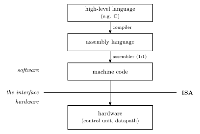
Figure 73: The ISA as an interface. Software above the line is written and compiled without knowing how the hardware works; hardware below the line is designed without knowing what program will run. The only thing both sides must agree on is which bit patterns mean what — and that agreement is a document, not a circuit.
The point of drawing it as a line is that the ISA is the only thing the two sides have to agree on. A compiler writer needs the ISA and nothing else about the chip; a chip designer needs the ISA and nothing else about the programs that will run.
Microarchitecture
Microarchitecture = the architecture of the control unit — i.e. the state machine (gates and flip-flops etc.) that implements the control unit.
This is the same state-machines material from earlier in the course, applied at the scale of a whole processor: the control unit is a state machine whose job is to emit the right control signals, in the right order, for whatever the instruction register holds.
ISA vs microarchitecture
One ISA can be implemented by many different microarchitectures. The specification says what the bit patterns mean; it does not say how a chip must go about honouring them.
| ISA | Implemented by |
|---|---|
| 8086 | many processors, in different ways |
| Pentium | Pentium … Pentium IV … Core2Duo … i7 (each in different ways), various AMD devices, and other manufacturers |
This is why a program compiled decades ago still runs: the ISA held still while the microarchitecture beneath it was rebuilt many times over.
What makes an ISA?
Four things:
- Memory models
- Registers
- Instructions
- Data types
If you know all these details, you can write machine code that runs on the CPU and build the CPU.
This is the completeness test for a specification: both sides of the line in Figure 73 have to be constructible from the document alone, and nothing else about the chip may be needed by either.
1. Memory models
How does memory look to the CPU? Four issues decide it — addressable cell size, alignment, address spaces and endianness — treated in full in memory-models.
2. Registers
Two types of register:
- General purpose — used for temporary results etc. On AVR, r0–r31.
- Special purpose, e.g.
- Program Counter (PC)
- Stack pointer (SP)
- Input/Output registers — 224 of them on the ATmega324A, see avr-io-ports
- Status register — N, Z, C, V among others. Tanenbaum calls this the Program Status Word.
Some other registers are part of the microarchitecture, NOT the ISA — e.g. the Instruction Register (IR). The programmer doesn’t need to know about these, and can’t directly change or use them.
That distinction is the cleanest illustration of what an ISA actually is. The IR unquestionably exists and holds the instruction being executed (fetch-decode-execute-cycle) — but no instruction names it, so it is invisible to software and a chip designer is free to change or remove it. The PC is the opposite case: jmp writes it, so it has to be in the specification. Existing in the hardware is not the criterion; being reachable from an instruction is.
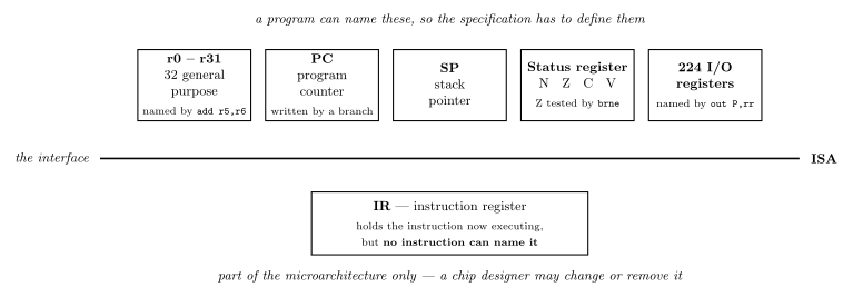
Figure 74: The same interface line as in the previous figure, with the machine’s registers sorted across it. The five above the line are part of the ISA; four of them carry an example of an instruction that names the register, and the SP box carries none. The single box below, the IR, is part of the microarchitecture only. Nothing about a register’s size or importance decides which side it lands on — only whether some instruction can refer to it.
The AVR’s own answer to this pillar — the regularity of r0–r31, the r16–r31 exception, and the X/Y/Z pointer pairs — is in avr-architecture.
3. Instructions
This is the main feature of an ISA. Instruction types include:
| Type | Does |
|---|---|
| Input/Output | communicate with I/O devices/ports |
| Load/Store | move data from/to memory |
| Move | copy data between registers |
| Arithmetic | addition, subtraction, … |
| Logical | Boolean operations |
| Branching | for deciding which instruction to perform next |
The Input/Output row is the one where the AVR’s answer is least obvious. The ATmega324A’s 224 I/O registers are all reachable by ld/st at their data-memory addresses 32 to 255 ($20 to $FF), but only the first 64 also get the short in rd, P / out P, rr form that names an I/O register by its own number P — because P is a six-bit field and \(2^6 = 64\). The other 160, the “extended” I/O registers, can only be reached the long way. The mechanics, the numbering offset and the register list are in avr-io-ports.
With arithmetic and logical merged, the same set can be cut the other way instead — by how many operands an instruction takes:
- Dyadic — two operands, one result
- Monadic — one operand, one result
And instructions use various addressing modes: how an operand says where its value is, covered in addressing-modes.
The AVR instructions met so far, sorted into these boxes, are in avr-instructions.
4. Data types
Numeric
- Integers of different lengths (8, 16, 32, 64 bits), possibly signed or unsigned
- Floating point numbers, e.g. 32 bits (single precision) or 64 bits (double precision)
- Many others not listed
Non-numeric
- Boolean (0 means false, 1 means true) — stored in a whole byte or word
- Bit-map (collection of Booleans, e.g. 8 in a byte)
- Characters
- Pointers (memory addresses)
Different machines provide hardware support for different data types. Two ends of the range:
Intel-64 Architecture
| Data type | 8 bits | 16 bits | 32 bits | 64 bits | 128 bits |
|---|---|---|---|---|---|
| Signed integer | \(\checkmark\) | \(\checkmark\) | \(\checkmark\) | \(\checkmark\) | |
| Unsigned integer | \(\checkmark\) | \(\checkmark\) | \(\checkmark\) | \(\checkmark\) | |
| BCD integer | \(\checkmark\) | ||||
| Floating point | \(\checkmark\) | \(\checkmark\) |
Atmel AVR
| Data type | 8 bits | 16 bits | 32 bits | 64 bits | 128 bits |
|---|---|---|---|---|---|
| Signed integer | \(\checkmark\) | ||||
| Unsigned integer | \(\checkmark\) | ||||
| BCD integer | |||||
| Floating point |
The only data type an AVR supports in hardware is an 8-bit integer, signed or unsigned. There is no 16-bit integer type, no floating point, no BCD.
Other data types can be supported through software! e.g. 16-bit integer operations can be built out of 8-bit operations, using a sequence of instructions — which is exactly what the two-instruction 16-bit addition in avr-instructions does. So the hardware/software line here is about cost, not possibility: anything missing from the table can still be computed, it just takes more instructions and more cycles. Floating point is the costly case: one float multiply is hundreds of instructions (floating-point-numbers), which is why fractions on the AVR are usually kept as fixed-point-numbers.
Assembly language
Machine code is too hard to program in. Assembly language is used instead:
- Human readable (just!).
- Converted into machine code by software called an assembler.
Two Atmel AVR examples:
| Assembly | Meaning |
|---|---|
add r3,r4 |
r3 ← r3 + r4 |
inc r22 |
r22 ← r22 + 1 |
The important structural detail is in the arrows of Figure 73: a high-level language compiles one-to-many — one line of C becomes however many instructions it takes — whereas assembly assembles one-to-one. Each assembly instruction is one machine instruction, written in a form a person can read. That is the whole of what an assembler buys you, and it is why assembly is still “programming the machine” in a way C is not.
The toolchain
For CSSE2010 the assembler is Microchip Studio, and two supplied tutorials walk through it end to end: Intro to Microchip Studio (create an assembler project, pick the device, edit, build, and step through the simulator) and Microchip Studio C Tutorial (the same for a GCC C project). Both are click-through guides to follow at the machine rather than material to learn — they are on Blackboard, and the labs are where they get used.
See also
- memory-models · addressing-modes — pillars 1 and 3, in full
- cpu-organisation · fetch-decode-execute-cycle · state-machines
- avr-architecture · avr-instructions · avr-io-ports · avr-program-structure
- assembly-process — what the assembler does besides translating: directives, segments and two passes · compilation-and-linking — the compiler’s one-to-many road, through object files and the linker
- 2026-08-27-avr-introduction — Lecture 10
- 2026-08-31-instruction-set-architecture-part-1 — Lecture 11
- 2026-09-03-instruction-set-architecture-part-2 — Lecture 12
Logic Gates
Every logic gate has one or more inputs and exactly one output, and can be described four equivalent ways: logic symbol, truth table, Boolean expression, timing diagram (see timing-diagrams for the last of these, and for real-gate propagation delay / rise / fall times).
Gates sit at the bottom of the abstraction stack — the digital logic level, level 0 (see 2026-07-27-course-intro-bits-bytes-binary). A digital circuit only ever carries two logic levels: logic ‘0’ is usually a small voltage (around 0 V) and logic ‘1’ a larger one (e.g. 0.8 V to 5 V, depending on the logic family — the type and size of the transistors the gate is built from). Because inputs and outputs have only these two states, they can equivalently be called true and false.
The 7 basic gate types
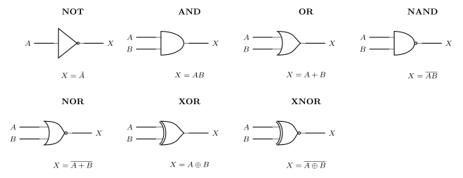
Figure 75: The seven basic gates, with the distinguishing symbol and Boolean expression for each. NOT, AND and OR are the three base shapes; NAND, NOR and XNOR are those same bodies with an inversion bubble on the output, and XOR/XNOR add a second arc across the back of the OR body.
| Gate | Behaviour | Truth table (\(A,B \to X\)) |
|---|---|---|
| NOT (inverter) | Inverts the input | 0→1, 1→0 |
| AND | Output is HIGH when all inputs are HIGH | 00→0, 01→0, 10→0, 11→1 |
| OR | Output is HIGH when at least one input is HIGH | 00→0, 01→1, 10→1, 11→1 |
| NAND | Output is HIGH when at least one input is LOW | 00→1, 01→1, 10→1, 11→0 |
| NOR | Output is HIGH when all inputs are LOW | 00→1, 01→0, 10→0, 11→0 |
| XOR | Output is HIGH when exactly one input is HIGH | 00→0, 01→1, 10→1, 11→0 |
| XNOR | Output is HIGH when the inputs are the same | 00→1, 01→0, 10→0, 11→1 |
Useful to remember: XOR is the odd function, XNOR is the even function.
Deriving the inverting gates from the base gates
The quickest way to fill in a NAND/NOR/XNOR truth table is not to memorise it, but to write the underlying AND/OR/XOR column first and then invert it row by row — the “N” prefix is exactly one inversion on the output:
| \(A\) | \(B\) | AND | NAND | OR | NOR | XOR | XNOR |
|---|---|---|---|---|---|---|---|
| 0 | 0 | 0 | 1 | 0 | 1 | 0 | 1 |
| 0 | 1 | 0 | 1 | 1 | 0 | 1 | 0 |
| 1 | 0 | 0 | 1 | 1 | 0 | 1 | 0 |
| 1 | 1 | 1 | 0 | 1 | 0 | 0 | 1 |
More than two inputs
A gate of \(n\) inputs has a truth table of \(2^n\) rows — two inputs give \(2 \times 2 = 4\) rows, three inputs give 8. The “at least one / all” wordings above carry over unchanged to more inputs; the XOR/XNOR wordings do not, and must be restated in terms of parity:
- XOR output is HIGH when an odd number of inputs are HIGH (the odd function). For two inputs this collapses to “exactly one”, which is why the 2-input wording works.
- XNOR output is HIGH when an even number of inputs are HIGH (the even function).
| \(A\) | \(B\) | \(C\) | 3-input AND | 3-input NAND | 3-input XOR |
|---|---|---|---|---|---|
| 0 | 0 | 0 | 0 | 1 | 0 |
| 0 | 0 | 1 | 0 | 1 | 1 |
| 0 | 1 | 0 | 0 | 1 | 1 |
| 0 | 1 | 1 | 0 | 1 | 0 |
| 1 | 0 | 0 | 0 | 1 | 1 |
| 1 | 0 | 1 | 0 | 1 | 0 |
| 1 | 1 | 0 | 0 | 1 | 0 |
| 1 | 1 | 1 | 1 | 0 | 1 |
Note that the kit of parts used for practicals has no 3-or-more-input gate chips (see device-pinouts) — a 3-input function has to be built from 2-input gates.
Universal (complete) gates
All circuits can be constructed from NAND-only or NOR-only gates — these are called complete (or universal) gates, because NOT, AND, and OR can each be built purely from one gate type:
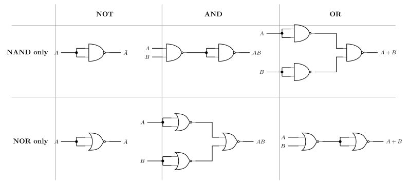
Figure 76: Why NAND and NOR are complete gates: NOT, AND and OR built from each one alone. Tying both inputs of a NAND or NOR together turns it into an inverter, and everything else follows — AND is NAND then invert, OR is invert-both-inputs then NAND (and the NOR row is the mirror image of that).
- NOT: a NAND (or NOR) gate with both inputs tied together — \(\overline{A \cdot A} = \bar A\), and \(\overline{A + A} = \bar A\).
- AND from NAND: a NAND followed by a second NAND wired as an inverter. AND from NOR: invert both inputs first, then NOR them (\(\overline{\bar A + \bar B} = AB\), by De Morgan — see boolean-algebra).
- OR from NOR: a NOR followed by a NOR-as-inverter. OR from NAND: invert both inputs first, then NAND them (\(\overline{\bar A \cdot \bar B} = A+B\)).
The two rows are De Morgan’s law drawn twice: whenever you push an inversion through a gate, AND and OR swap. NAND and NOR are preferred in practice because they are easier to build from transistors than AND/OR directly.
Gates on ICs
Gates are sold packaged several to an integrated circuit (IC). The 74HCT00 is four independent 2-input NAND gates in one 14-pin DIP package.
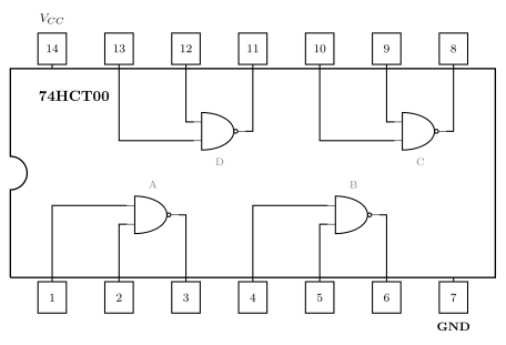
Figure 77: Inside the 74HCT00: four independent 2-input NAND gates in a 14-pin package, with the pin each gate terminal is wired to. Pin 14 is Vcc (power, e.g. 5 V) and pin 7 is GND (0 V) — shared by all four gates, so nothing works if either is left unconnected. Gate letters A-D are the labels a schematic uses as U1:A … U1:D.
- Vcc = power (e.g. 5 V), GND = ground (0 V). One Vcc/GND pair supplies all four gates.
- Physically: pin spacing is 0.1” along the package and 0.3” across it; the chip is about 15 mm long.
- The drawing above is the chip’s internal schematic, not a picture of the part — see circuit-schematics for how a chip like this is drawn (and labelled
U1:A…U1:D) on a schematic you can actually build from, and device-pinouts for the pinouts of every chip in the course kit.
Sequential Circuits
A sequential circuit is a circuit whose output depends not only on the current inputs but also on the values it is currently storing. The storage is done with flip-flops — see flip-flops-and-latches for the storage elements themselves.
The output of any logic gate or combinational circuit depends on the current value of the inputs only, so if an input changes, the output can change too and the previous value is lost forever. A circuit with memory can remember a value even when the input changes. First met in 2026-08-10-introduction-to-sequential-circuits.
Combinational vs sequential
| Combinational | Sequential | |
|---|---|---|
| Contents | Logic gates only (no flip-flops) | Includes flip-flops as well as logic gates |
| Output determined by | The inputs alone — uniquely | Current inputs and current state |
| Repeatability | Same inputs always give the same output | Same inputs can give different outputs, depending on state |
| When output changes | Whenever an input changes | Only when the clock ‘ticks’ |
| Examples | Adders, multiplexers, decoders, demultiplexers, encoders (see combinational-logic-blocks) | Counters, registers (see [counters], shift-registers) |
The two example lists are worth memorising as the dividing line: the blocks built earlier in the course are all combinational, and the ones that follow — registers, counters, state machines — are all sequential.
A combinational example from earlier in the course: \(A\) into one input of an AND gate, \(B\) and \(C\) into an OR gate whose output feeds the AND gate’s other input, giving \(X = A(B+C)\). Nothing in that circuit remembers anything — change \(A\), \(B\) or \(C\) and the output follows immediately (after propagation delay; see timing-diagrams).
The key contrast: if an input to a combinational circuit changes, the output can change too and the previous value is lost forever. A sequential circuit can hold onto a value even after the input that produced it has gone away.
State
- State = the value stored in the flip-flops.
- Output depends on the inputs and the state.
- Next state depends on the inputs and the (present) state.
“Present state” is what the flip-flops hold right now; “next state” is what they will hold after the next clock edge. The combinational logic computes the next state from the present state and the inputs; the flip-flops only adopt it when the clock edge arrives.
General structure of a sequential circuit
The standard block diagram has two blocks and a feedback loop.
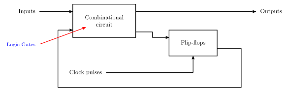
Figure 78: The general sequential circuit (after Mano, Digital Design, 3rd edition). Two things carry the whole idea: the loop running from the flip-flops back into the combinational block, which is what makes the circuit sequential, and the clock stub, which enters the flip-flops and nothing else. The ‘Logic Gates’ callout marks the combinational block as gates only.
- A combinational circuit block (just logic gates). It takes the external inputs plus the feedback from the flip-flops, and produces the external outputs plus the values to be loaded into the flip-flops.
- A flip-flops block (the storage elements). Its data inputs come from the combinational circuit; it also takes clock pulses as a separate control input.
- A feedback path runs from the flip-flops’ outputs back around into the combinational circuit’s inputs. That loop is what makes the circuit sequential — the stored state is fed back in and influences the next output and the next state.
The clock pulses go only to the flip-flops, not to the combinational logic. Cut the feedback wire and what is left is a plain combinational circuit with a register bolted on the end; it is the loop that makes the difference.
This same block diagram reappears in shift-registers, [counters] and state-machines — those are all just specific choices of what goes in the combinational block.
Synchronous sequential circuits
In a synchronous sequential circuit the storage elements can only change at discrete instants of time, set by a common clock signal.
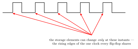
Figure 79: A clock signal. The five arrows all point at rising edges: these are the only instants at which any storage element in a synchronous circuit is allowed to change. Everywhere else on the axis the flip-flops are inert, however much their inputs move — which is exactly the opposite of a logic gate, whose output changes whenever its input does.
- Assume a clock signal — a regularly repeating train of pulses alternating between 0 and 1.
- The outputs of the storage elements change only on the edges of that control signal.
- Contrast with logic gates, whose outputs change whenever their inputs change.
Because every flip-flop shares the same clock, the whole circuit’s state changes in one step at each clock edge, which is what makes such circuits tractable to design and analyse.
It also means the clock period sets the pace of the design: everything the combinational block has to compute must settle within one tick. This follows from the propagation delays of timing-diagrams.
See also
- 2026-08-10-introduction-to-sequential-circuits — Lecture 5
- state-machines — the same circuits described by their states and transitions, which is how they are actually designed.
- flip-flops-and-latches · [counters] · shift-registers
- csse2010-diagram-notation — the block-diagram conventions the figures above follow
State Machines
A state machine — equivalently a finite state machine (FSM) — is another name for a sequential circuit, viewed in terms of the states it can be in rather than the gates and flip-flops that implement it. See sequential-circuits for the circuit-level view and flip-flops-and-latches for the storage elements the state lives in.
What a state machine is
A state machine has:
- a finite number of possible states — \(N\) flip-flops give at most \(2^N\) of them;
- only one current state at any moment;
- the ability to transition to other states, based on the inputs and the current state.
The state is exactly the value held in the flip-flops (see sequential-circuits), so the flip-flop count bounds the state count. It does not fix it: how many flip-flops a given number of states actually costs is an encoding choice, made at the state-encoding step below.
Naming the two blocks of logic
The standard sequential-circuit structure has one combinational block computing two different things, and it is worth naming them separately:
\[\text{OUT} = g(\text{IN}, Q) \qquad\qquad D = f(\text{IN}, Q)\]
- \(Q\) is the present state (PS) — what the flip-flops hold right now.
- \(D\) is the next state (NS) — what they will hold after the next clock edge.
- \(g\) is the output logic; \(f\) is the transition logic (also called next-state logic).
Designing an FSM comes down to finding Boolean expressions for \(f\) and \(g\).
Defining the states from the problem
States are not handed to you — they come from the problem, and the useful question is what does the circuit need to remember?
Vending machine. A machine accepts 5c and 10c coins and dispenses a candy when it has received 15 cents in total. What are the states?
What the machine must remember is the running total inserted so far:
| Total inserted | 0 | 5 | 10 | 15 | 20 | 50 |
|---|---|---|---|---|---|---|
| Dispense candy? | no | no | no | yes | yes, plus change | — |
So the states are the totals 0, 5 and 10, with 15 and 20 being the ones that dispense (20 arises from inserting 10c on top of 10c, and needs change). A total of 50 is not a state at all: with only 5c and 10c coins the machine dispenses and resets long before it could get there, so it is unreachable.
Moore and Mealy machines
There are two types, differing only in what the output logic is allowed to see:
- Mealy machine — outputs depend on the current state and the inputs.
- Moore machine — outputs depend only on the current state (the flip-flop values). Consequently, outputs can only change when the state changes.
A Moore machine is a special case of a Mealy machine — the one where the output logic simply ignores its input connections. CSSE2010 sticks to Moore machines.
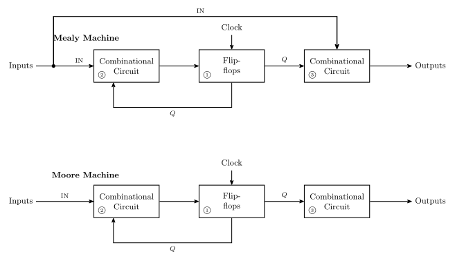
Figure 80: Mealy (top) and Moore (bottom). ① is the state, held in the flip-flops; ② is the transition logic; ③ is the output logic. The only structural difference is the branch drawn in bold: in a Mealy machine the inputs reach the output logic directly, so the outputs are a function of IN and Q; in a Moore machine the output logic sees Q alone.
State diagram notation
A state diagram draws the states as circles and the transitions as labelled arrows.
States are drawn as a circle split in two: the state name on top, the output value(s) underneath. So \(S_0\) over \(101\) is a state called \(S_0\) whose outputs are 101; the name is arbitrary and need not be \(S_n\) (a state called Alex over \(01\) is just as legal).
Transitions are arrows labelled with a logic expression over the inputs — if the expression is true, that transition is taken. Examples of labels: \(Z\), \(\overline{\text{RESET}}\), \(A + B\cdot\overline{C}\).
Two conventions worth knowing:
- No label means “true” — the transition is always taken on the next clock edge. This is what the arrows in a plain counter’s diagram look like.
- With only one input, the label may be written as just
0or1instead of a Boolean expression. This is a special case of the general form; \(1\) means the same as \(Z\) and \(0\) the same as \(\overline{Z}\).
Completeness
Each possible combination of inputs should be addressed exactly once for each state.
That is, the transition arrows leaving each state must encompass all possibilities, without overlap and without gaps. With \(N\) inputs there are \(2^N\) input combinations, so every state needs \(2^N\) transitions accounted for — though several combinations leading to the same next state can be merged onto one arrow with an OR’d label.
This is a checkable property, and checking it is the cheapest way to catch a half-finished design: if the labels on the arrows out of a state do not OR together to 1, some input combination has no defined behaviour; if any two of them can be true at once, the machine is ambiguous.
A counter is a state machine with no inputs
The design method for counters — write the sequence as a present-state/next-state table, read each \(D\) column off as a Boolean function of the \(Q\)’s, draw the gates — is steps 3, 5 and 6 of the pipeline below, applied to the degenerate case where the machine has no external inputs at all. A counter may or may not have external inputs.
Three things collapse when \(\text{IN}\) is empty:
- Transition logic. \(D = f(\text{IN}, Q)\) becomes \(D = f(Q)\), so the state table needs no input column and the excitation equations are functions of the \(Q\)’s alone.
- Output logic. A counter’s output is its state, so \(g\) is the identity and there is no second block of gates. That also makes every counter trivially a Moore machine.
- Completeness. With \(N = 0\) inputs there are \(2^0 = 1\) input combinations, so the completeness rule reduces to exactly one arrow out of each state — and by the “no label means true” convention, that arrow is unlabelled.
The state encoding step also disappears, or rather it is made for you: the states of a counter are already bit patterns, and the sequence you were given is the encoding.
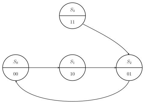
Figure 81: The 2-bit counter for \(00 \to 10 \to 01 \to 00\) drawn as a state diagram. Every arrow is unlabelled because the machine has no inputs, so each transition is taken unconditionally on the next clock edge; each state’s output half carries the count value, since a counter’s output is its state. \(S_3\) is the unused state: three states cannot fill a two-flip-flop machine, so its next state is a don’t-care, and choosing \(11 \to 01\) for it is what makes the design self-correcting.
Figure 81 read as a state table, with the unused row carrying the don’t-cares:
| Current state | Next state | \(Q_1\) | \(Q_0\) |
|---|---|---|---|
| \(S_0\) | \(S_1\) | 0 | 0 |
| \(S_1\) | \(S_2\) | 1 | 0 |
| \(S_2\) | \(S_0\) | 0 | 1 |
| \(S_3\) | (don’t care) | 1 | 1 |
The unused state is where the FSM framing pays for itself. A don’t-care is a free choice of transition, not an absence of one: the circuit will do something in state \(S_3\), and the only question is whether the arrow you have implicitly drawn leads back into the cycle or loops onto itself. An arrow from \(S_3\) to itself is a trap state — the machine leaves the intended cycle and never returns. There are two candidate simplifications for \(D_1\). The tidier one, \(D_1 = \overline{Q_1 \oplus Q_0}\), puts a self-loop on \(S_3\) and is rejected. The other sends \(11 \to 01\), back into the cycle, and is the robust design. See [counters] and 2026-08-17-counters for that working.
State tables
The same information as a state diagram, in tabular form. Two layouts, both in use.
One-dimensional — one row for every combination of state and inputs:
| Current State | Input \(U\) | Next State | \(Q_1\) | \(Q_0\) |
|---|---|---|---|---|
| \(S_0\) | 0 | \(S_3\) | 0 | 0 |
| \(S_0\) | 1 | \(S_1\) | 0 | 0 |
| \(S_1\) | 0 | \(S_0\) | 0 | 1 |
| \(S_1\) | 1 | \(S_2\) | 0 | 1 |
| \(S_2\) | 0 | \(S_1\) | 1 | 0 |
| \(S_2\) | 1 | \(S_3\) | 1 | 0 |
| \(S_3\) | 0 | \(S_2\) | 1 | 1 |
| \(S_3\) | 1 | \(S_0\) | 1 | 1 |
Two-dimensional — one row per state, with a next-state column for every combination of inputs:
| Current State | Next State (\(\overline{U}\)) | Next State (\(U\)) | \(Q_1\) | \(Q_0\) |
|---|---|---|---|---|
| \(S_0\) | \(S_3\) | \(S_1\) | 0 | 0 |
| \(S_1\) | \(S_0\) | \(S_2\) | 0 | 1 |
| \(S_2\) | \(S_1\) | \(S_3\) | 1 | 0 |
| \(S_3\) | \(S_2\) | \(S_0\) | 1 | 1 |
Both describe the same machine (a 2-bit up/down counter, \(U = 1\) counts up). The 2D form is more compact and makes completeness visually obvious — every input combination is a column, so a missing case is a missing column. The 1D form grows as \(2^N \times\) (number of states) but maps directly onto a truth table, which is what the next design step needs. In a Moore machine the output columns depend only on the current state, which is why they can sit in a per-state row at all.
State encoding
Each state must be encoded into flip-flop values before the design can become a circuit. Two choices to make:
- the number of flip-flops, and
- the bit patterns representing each state.
Ideally, choose the encoding that makes the combinational logic simple — for both the output logic and the next-state logic. Different encodings of the same machine give genuinely different gate counts.
Three common schemes, on a four-state machine:
| State | Binary | Gray | One-hot |
|---|---|---|---|
| \(S_0\) | 00 | 00 | 0001 |
| \(S_1\) | 01 | 01 | 0010 |
| \(S_2\) | 10 | 11 | 0100 |
| \(S_3\) | 11 | 10 | 1000 |
- Binary — the obvious count; \(\lceil \log_2 n \rceil\) flip-flops for \(n\) states.
- Gray — same width, but consecutive states differ in exactly one bit (see binary-number-representations).
- One-hot — one flip-flop per state, with only one flip-flop holding 1 at any time. Far more flip-flops, but the next-state and output logic often collapses to almost nothing, since “am I in state \(S_k\)” is just a single flip-flop’s output rather than a decoded combination.
Steps involved in FSM design
- Defining state based on the problem definition.
- Drawing the state diagram.
- Completing the state table (1D or 2D).
- State encoding, and re-doing the state table with encoded states.
- Obtaining the Boolean expressions for the next-state logic (i.e. the \(D\)’s) and for the outputs.
- Drawing the logic diagram.
- Simulating in Logisim to verify functionality.
- Building and testing the circuit in hardware.
Steps 1–6 are the pen-and-paper design; steps 7–8 are what the learning labs do with it. Steps 5 and 6 are the same techniques used to build a counter by hand — see [counters] and circuit-schematics.
See also
- sequential-circuits · flip-flops-and-latches · [counters] · shift-registers
- 2026-08-17-counters — Lecture 7, where this design method is first used (on counters)
- 2026-08-20-state-machines — Lecture 8
- week9-lab-avr-interrupts — Lab 14: a stopwatch controller designed as a Moore machine and written in C