CSSE2010 — Week 12 Notes
Lecture 23 — Floating Point Numbers
How a computer stores fractions, and numbers far too large or too small for any sensible number of integer bits. The note starts from why that is needed, with the number of air molecules in a coffee cup; covers fixed point, where the binary point sits at an agreed place, and the trade-off between range and precision it forces; then lets the point float, by way of scientific notation, normalisation and the log-table origin of the word “mantissa”; and then works through the IEEE 754 single and double precision formats, converting in both directions, finite precision and what it does to arithmetic, the formats from quarter to octuple precision, the special values zero, subnormal, infinity and NaN, and floating point in C and on the AVR. The reference notes are fixed-point-numbers and floating-point-numbers. Whole-number formats, including the excess notation the exponent uses, are in binary-number-representations.
Goals
- See why a fixed number of integer bits cannot hold both very large and very small quantities.
- Represent fractions in fixed point: convert a value to an \(m.n\) format and read a bit pattern in one, unsigned and two’s complement, and state the range and precision of every 8-bit format.
- Write numbers in normalised scientific notation, in decimal and in binary, and say where the word “mantissa” comes from.
- Describe the IEEE 754 single and double precision formats: the fields, the biased exponent, the implicit leading 1, and why the fields are in that order.
- Convert a decimal number to IEEE single precision in hexadecimal, and back.
- Explain the limits of floating point: finite precision and its effect on arithmetic, the special values, and how the formats from quarter to octuple precision compare.
- Know how C and the AVR handle floating point, and why integer arithmetic is preferred on the AVR.
The problem: how many molecules in a cup?
Worked: air molecules in an empty coffee cup
How many air molecules are in an empty 12 fl oz coffee cup at 1 atm and 26.85 °C?
The ideal gas law, \(pV = nRT\), gives the amount of gas \(n\) in moles. In SI units, rounded to keep the arithmetic simple:
| Quantity | Given | SI, rounded |
|---|---|---|
| pressure \(p\) | 1 atm | \(100\,000\) Pa |
| volume \(V\) | 12 fl oz | \(0.00036\ \text{m}^3\) |
| gas constant \(R\) | \(8\ \text{J/(K·mol)}\) | |
| temperature \(T\) | 26.85 °C | \(300\) K |
\[n = \frac{pV}{RT} = \frac{100\,000 \times 0.00036}{8 \times 300} = \frac{36}{2400} = 0.015\ \text{mol}.\]
Molecules = \(n \times\) Avogadro’s number, \(N_A = 6.02214076 \times 10^{23}\) = 602214076000000000000000:
\[0.015 \times 602\,214\,076\,000\,000\,000\,000\,000 = 9\,033\,211\,140\,000\,000\,000\,000 \approx 9.03 \times 10^{21}.\]
(The roundings are generous: 1 atm is 101 325 Pa, 12 US fl oz is \(0.000355\ \text{m}^3\) and \(R\) is 8.314. With those, \(n \approx 0.0144\) mol and the count is about \(8.7 \times 10^{21}\). Either way only the first two or three digits mean anything.)
What this says about storing numbers. Avogadro’s number needs 79 bits as an integer, and the answer 73. The volume, \(0.00036\), has its first 1 only in the 12th place after the binary point (\(2^{-12} \approx 0.000244\)), so it needs at least 12 fractional bits to register at all. A format that held all three exactly would need about 80 integer bits and a few dozen fractional bits, almost all of them zero in any one value, and every digit past the third would be noise anyway. What is worth storing is the significant digits and the scale, separately. That is floating point, and the stepping stone to it is fixed point.
Fractions in binary: fixed point
Place values continue past the binary point by halving: \(2^{-1} = \tfrac12\), \(2^{-2} = \tfrac14\), \(2^{-3} = \tfrac18\), \(2^{-4} = \tfrac1{16}\). Fixed-point notation chooses a place for the point, arbitrarily, and keeps it there. The point is never stored; it is an agreement about how to read the bits.
| \(2^3\) | \(2^2\) | \(2^1\) | \(2^0\) | . | \(2^{-1}\) | \(2^{-2}\) | \(2^{-3}\) | \(2^{-4}\) |
|---|---|---|---|---|---|---|---|---|
| 8 | 4 | 2 | 1 | . | \(\tfrac12\) | \(\tfrac14\) | \(\tfrac18\) | \(\tfrac1{16}\) |
A format with \(m\) integer bits and \(n\) fractional bits is called \(m.n\). The full treatment is fixed-point-numbers.
Worked: representing 4.375
How is 4.375 represented in 8-bit fixed point, with 4, 5 or 3 integer bits?
Whole part: \(4 = 100_2\).
Fraction, by repeated doubling: \(0.375 \times 2 = 0.75\) (bit 0), \(0.75 \times 2 = 1.5\) (bit 1), \(0.5 \times 2 = 1.0\) (bit 1), and the fraction is now 0. Reading the bits in the order they came: \(0.375 = 0.011_2\). As a check by subtraction, \(0.375 - 0.25 = 0.125 = \tfrac18\), so the \(\tfrac14\) and \(\tfrac18\) bits are set.
Or all at once: with 3 fractional bits, every value is a whole number of eighths. \(4.375 \times 8 = 35 = 100011_2\); put the point back three places from the right: \(100.011_2\).
So \(4.375 = 100.011_2\), and in each format:
| Format | Bits |
|---|---|
| 4.4 | 0100.0110 |
| 5.3 | 00100.011 |
| 3.5 | 100.01100 |
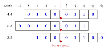
Figure 1: The value 4.375 in three 8-bit fixed-point formats. The significant bits 1, 0, 0, 0, 1, 1 are the same every time; each lines up with the same place values, 4, 1/4 and 1/8, wherever the point is put. Moving the point one place left therefore shifts the bits one place left in the byte, a 0 dropping off the left end and a 0 joining on the right. The format decides which values fit: 4.375 needs at least 3 integer bits and 3 fractional bits, and all three formats here have that.
Worked: 10110101 as unsigned 5.3
What does the 8-bit number
10110101represent in unsigned fixed-point notation with 5 integer bits and 3 fractional bits?
Split it 5 and 3: 10110.101.
- Integer bits
10110\(= 16 + 4 + 2 = 22\). - Fraction bits
.101\(= \tfrac12 + \tfrac18 = 0.625\).
Answer: 22.625. Check: read as a whole number the byte is 181, and \(181 / 2^3 = 22.625\).
Worked: 10110101 as two’s complement 5.3
What does the same
10110101represent in two’s complement fixed-point notation with 5 integer bits and 3 fractional bits? Choices: \(-9.375\), \(-10.625\), \(-9.625\).
In two’s complement the MSB’s weight is negative (binary-number-representations). In 5.3 the MSB is worth \(-2^4 = -16\), and every other bit keeps its positive weight, fraction bits included:
\[\underbrace{-16}_{1} + \underbrace{0}_{0} + \underbrace{4}_{1} + \underbrace{2}_{1} + \underbrace{0}_{0}\ .\ \underbrace{\tfrac12}_{1} + \underbrace{0}_{0} + \underbrace{\tfrac18}_{1} = -10 + 0.625 = -9.375.\]
Answer: \(-9.375\). Two checks:
- Unsigned it was 22.625. A set MSB in two’s complement subtracts \(2^5 = 32\) from the unsigned reading: \(22.625 - 32 = -9.375\).
- Negate it: invert every bit,
01001.010\(= 9.25\), and add 1 in the last place, \(\tfrac18\): \(9.375\). So the original is \(-9.375\).
Where the other two come from:
- \(-10.625\) reads the integer bits correctly as \(-10\) and then attaches the fraction as if it shared the sign, \(-(10 + 0.625)\). But the fraction bits have positive weight: \(-10 + 0.625 = -9.375\).
- \(-9.625\) inverts only the integer bits (
10110→01001= 9) and keeps.101as it is. That is neither rule: negating needs every bit inverted and then a 1 added in the last place.
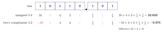
Figure 2: One byte, 10110101, read in two 5.3 formats. The weights are identical except for the MSB, which is worth +16 unsigned and -16 in two’s complement. Summing the weights of the 1 bits (the weights of the 0 bits are greyed out) gives 22.625 unsigned and -9.375 two’s complement, and the two differ by exactly 32, twice the MSB’s weight. The fraction bits add 1/2 and 1/8 in both readings: a two’s complement fraction is never subtracted.
Range against precision
Every 8-bit format has the same 256 patterns; the format only spaces them. For unsigned \(m.n\) the precision is the last bit’s weight, \(2^{-n}\), and the maximum is all ones, \(255 \times 2^{-n}\):
| Format | Maximum | Precision | Format | Maximum | Precision | |
|---|---|---|---|---|---|---|
| 8.0 | 255 | 1 | 4.4 | 15.9375 | 0.0625 | |
| 7.1 | 127.5 | 0.5 | 3.5 | 7.96875 | 0.03125 | |
| 6.2 | 63.75 | 0.25 | 2.6 | 3.984375 | 0.015625 | |
| 5.3 | 31.875 | 0.125 | 1.7 | 1.9921875 | 0.0078125 | |
| “9.$-\(1" | 510 | 2 | | 0.8 | 0.99609375 | 0.00390625 | | "10.\)-$2” | 1020 | 4 |
8.0 is xxxxxxxx. (an ordinary byte), 7.1 is xxxxxxx.x, 6.2 is xxxxxx.xx, and so on. Each place the point moves left halves both the maximum and the step. The formats in quotes go the other way: in “9.$-\(1" the point sits one place *beyond* the byte, `xxxxxxxx0.`, so the lowest stored bit is worth 2 and only even numbers up to 510 exist; "10.\)-$2” is xxxxxxxx00., multiples of 4 up to 1020. No choice of point gets range and precision together. Two’s complement ranges, and a drawing of the point sliding, are in fixed-point-numbers.
Letting the point move
Natural language and scientific notation
People handle the same problem with a variable decimal point. In words, SI prefixes move it: kilometre, milligram, femtometre, yoctogram, each prefix a power of 10. In symbols, scientific notation writes significant digits times a power of 10: Avogadro’s number is \(6.02 \times 10^{23}\), and the cup’s \(0.00036\ \text{m}^3\) is \(3.6 \times 10^{-4}\ \text{m}^3\). A few digits plus an exponent covers any size.
Normalisation
The same value can be written \(602 \times 10^{21}\), \(60.2 \times 10^{22}\), \(6.02 \times 10^{23}\) or \(0.602 \times 10^{24}\). Normalised means one non-zero digit before the point, the digits in \([1, 10)\), so \(6.02 \times 10^{23}\) is the normalised one: \(602 \times 10^{21}\) and \(60.2 \times 10^{22}\) have too many digits before the point, and \(0.602 \times 10^{24}\) has a zero there.
In binary the range is \([1, 2)\): the only non-zero binary digit is 1, so a normalised binary number is always \(1.xxx_2 \times 2^e\).
Worked: which two are correctly normalised in binary?
Which two of these values have the correct binary normalisation?
A. \(15.940 \times 2^{75}\) B. \(7.970 \times 2^{76}\) C. \(3.985 \times 2^{77}\) D. \(1.993 \times 2^{78}\) E. \(0.996 \times 2^{79}\)
F. \(11.796 \times 2^{-15}\) G. \(5.898 \times 2^{-14}\) H. \(2.949 \times 2^{-13}\) I. \(1.475 \times 2^{-12}\) J. \(0.737 \times 2^{-11}\)
Answer: D and I, the only two with the multiplier in \([1, 2)\).
The two rows are each one number written five ways: halving the multiplier and adding 1 to the exponent leaves the value unchanged. A to E are all \(\approx 6.02 \times 10^{23}\), Avogadro’s number; F to J are all \(\approx 3.60 \times 10^{-4}\), the volume of the cup in m³ (to the three decimals shown). Exactly one spelling of each is normalised.
| Option | Multiplier | Normalised in binary? | Why not |
|---|---|---|---|
| A | 15.940 | \(\times\) | \(\geq 2\): shift three more places |
| B | 7.970 | \(\times\) | \(\geq 2\): shift two more places |
| C | 3.985 | \(\times\) | \(\geq 2\): shift one more place |
| D | 1.993 | \(\checkmark\) | |
| E | 0.996 | \(\times\) | \(< 1\): a leading 0 |
| F | 11.796 | \(\times\) | \(\geq 2\) |
| G | 5.898 | \(\times\) | \(\geq 2\) |
| H | 2.949 | \(\times\) | \(\geq 2\) |
| I | 1.475 | \(\checkmark\) | |
| J | 0.737 | \(\times\) | \(< 1\): a leading 0 |
The trap is the decimal rule. B, C, G and H have one non-zero digit before the point, so they look normalised by the \([1, 10)\) rule. But the base here is 2, and with base 2 the multiplier must be in \([1, 2)\). E and J fail the other way: their leading digit is 0.
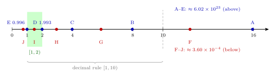
Figure 3: The ten multipliers on a number line, Avogadro’s number written five ways above the line and the cup’s volume five ways below. Each step left halves the multiplier and adds 1 to the power of 2, so the value stays the same. A binary normalised multiplier must lie in [1, 2), the shaded window, and exactly one spelling of each number lands in it: D, 1.993, and I, 1.475. E, at 0.996, sits just outside the left edge, and D just inside the right one. The wider window [1, 10) of decimal normalisation would wrongly admit B, C, G and H as well.
Why “mantissa”
The digits part of a floating-point number is called the mantissa, a name taken from logarithm tables. Logarithms turn multiplication into addition, \(\log(a \times b) = \log a + \log b\), and before calculators that was done with printed tables. A standard four-figure table gives the logarithms of 1.00 to 9.99: row 12, column 3 reads 0899, meaning \(\log_{10} 1.23 \approx 0.0899\).
Worked: three logarithms from one table entry
Given \(\log_{10} 1.23 \approx 0.0899\), what are \(\log_{10} 12.3\), \(\log_{10} 123\) and \(\log_{10} 0.123\)?
Each is \(1.23\) times a power of 10, and the log of a product is the sum of the logs:
- \(\log_{10} 12.3 = \log_{10} (1.23 \times 10) = 0.0899 + 1 = \mathbf{1.0899}\)
- \(\log_{10} 123 = \log_{10} (1.23 \times 10^2) = 0.0899 + 2 = \mathbf{2.0899}\)
- \(\log_{10} 0.123 = \log_{10} (1.23 \times 10^{-1}) = 0.0899 - 1 = \mathbf{-0.9101}\)
The fractional part, 0.0899, is the same every time and depends only on the digits 1, 2, 3: that was the mantissa. The integer part, 1, 2 or \(-1\), only places the point: that was the characteristic. (For \(0.123\), tables kept the mantissa visible by writing \(\bar{1}.0899\), meaning \(-1 + 0.0899\).) So the table only needs mantissas, and the power of 10 is handled by adding a whole number. A floating-point number splits the same way, digits and an exponent, and the digits took the old name.

Figure 4: Logarithms of 0.123, 1.23, 12.3 and 123 on a log scale. Each is ten times the one before, so each sits exactly one unit further along. Every logarithm splits into a whole number, the characteristic, plus the same fractional part, 0.0899, which depends only on the digits 1, 2, 3; that fractional part was called the mantissa. The characteristic only records the power of 10, which is to say where the point goes.
IEEE 754
The standard formats store a sign bit \(S\), an exponent field \(E\) and a mantissa field \(M\), and mean
\[(-1)^S \times 1.M_2 \times 2^{E - \text{bias}}.\]
- Single precision, 32 bits: 1 sign bit, 8 exponent bits in excess-127 format, 23 mantissa bits.
- Double precision, 64 bits: 1 sign bit, 11 exponent bits in excess-1023 format, 52 mantissa bits.
- The mantissa is normalised, so it begins with 1, and that 1 is implicit: it is not stored, which buys a 24th (or 53rd) significant bit. The exception is the subnormal numbers (below), where the hidden bit is 0.
Excess-127 means the field holds the true exponent plus 127. It is the excess notation of binary-number-representations, but with a bias one less than \(2^7 = 128\). The field layouts are drawn in floating-point-numbers.
Worked: why sign, then exponent, then mantissa?
Why are the fields in the order sign, exponent, mantissa?
So that floats compare like integers. Take \(1 \times 2^{100}\) and \(3 \times 2^{20}\). The first is far bigger despite the smaller leading number, because the exponent fixes the scale and the mantissa only refines it within that scale. Normalised, they are \(1.0_2 \times 2^{100}\) and \(1.1_2 \times 2^{21}\), with exponent fields \(100 + 127 = 227\) and \(21 + 127 = 148\). With the exponent in the high bits, comparing the two 32-bit patterns as unsigned integers compares 227 with 148 first and gets the right answer without looking at the mantissas. The mantissa only decides between numbers with equal exponents, which is exactly when it should.
The bias helps: in excess form larger exponents, negative ones included, are always larger unsigned fields. And the sign at the very top separates negatives from positives first. So the integer comparison circuits can sort non-negative floats directly.
Conversion steps
- Convert to binary scientific notation, normalised.
- Store the sign: \(+ \to 0\), \(- \to 1\).
- Store the biased exponent: true exponent \(+ 127\).
- Store the mantissa: drop the implicit 1 and right-pad with zeros to 23 bits.
Then group into nibbles for hex. And beware of special values: zero, infinity and NaN have reserved patterns.
Worked: \(-23.25\) to IEEE single precision
Convert \(-23.25\) to an IEEE single-precision floating-point number, expressed in hexadecimal.
1. Binary scientific notation. \(23 = 10111_2\) and \(0.25 = 0.01_2\), so \(23.25 = 10111.01_2\). Move the point four places left: \(10111.01_2 = 1.011101_2 \times 2^4\).
2. Sign. Negative, so \(S = 1\).
3. Exponent. \(4 + 127 = 131 = 10000011_2\).
4. Mantissa. Drop the leading 1: 011101, then pad with zeros on the right to 23 bits: 01110100000000000000000.
Assemble and group:
| S | Exponent | Mantissa |
|---|---|---|
1 |
10000011 |
01110100000000000000000 |
1100 0001 1011 1010 0000 0000 0000 0000 = C 1 B A 0 0 0 0, so \(-23.25\) = 0xC1BA0000.
Checks: \(+23.25\) differs only in the sign bit, 0x41BA0000. In double precision the exponent is \(4 + 1023 = 1027\) and the pattern 0xC037400000000000; in half precision (5-bit exponent, bias 15) it is 0xCDD0.
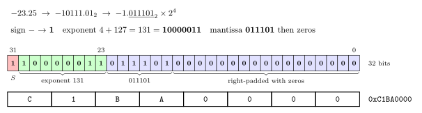
Figure 5: Encoding -23.25 in single precision. The minus sign becomes a 1 in the sign bit. The value 10111.01 in binary is normalised to 1.011101 times 2 to the 4, the 4 is stored as 4 + 127 = 131, and the bits after the leading 1 fill the mantissa field from the left, with zeros padding it out on the right. The 32 bits then group into nibbles from the left, giving C1BA0000 in hexadecimal. The nibble boundaries do not line up with the field boundaries: the C takes the sign and the first three exponent bits.
Worked: 0x422F0000 to decimal
Convert
0x422F0000from an IEEE floating-point number to a decimal value.
Bits. 4 2 2 F 0 0 0 0 = 0100 0010 0010 1111 0000 0000 0000 0000.
Split 1 / 8 / 23.
| S | Exponent | Mantissa |
|---|---|---|
0 |
10000100 |
01011110000000000000000 |
- Sign 0: positive.
- Exponent \(10000100_2 = 132\), not all 0s or all 1s, so normal; true exponent \(132 - 127 = 5\).
- Mantissa: put back the hidden 1: \(1.0101111_2\).
Value. \(+1.0101111_2 \times 2^5\): move the point five places right, \(101011.11_2 = 32 + 8 + 2 + 1 + \tfrac12 + \tfrac14 = \mathbf{43.75}\).
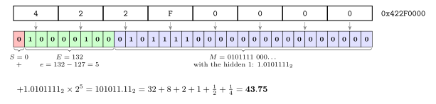
Figure 6: Decoding 0x422F0000. Each hex digit expands to four bits, and the 32 bits are then cut at the field boundaries, which fall in the middle of the first three hex digits. The sign bit 0 means positive. The exponent field 10000100 is 132, so the true exponent is 132 - 127 = 5. The mantissa field gets its hidden 1 back in front, giving 1.0101111, and shifting the point five places right gives 101011.11, which is 43.75.
Finite precision
Not every number can be represented precisely. A float has a fixed number of mantissa bits, so a value that needs more is rounded, and rounding happens again after every operation.
Worked: does \((10.0 \div 3) \times 3\) give 10.0?
Is \((10.0 \div 3) \times 3\) equal to \(10.0\) in floating point?
\(10 \div 3 = 3.333\ldots = 11.010101\ldots_2\), with 01 repeating for ever, so the stored quotient is cut short and is not exactly \(\tfrac{10}{3}\). In 3-digit decimal the effect is plain: \(10.0 \div 3 = 3.33\), and \(3.33 \times 3 = 9.99\).
In binary it depends on how the two roundings fall. For this particular case they cancel, and single and double precision both give exactly 10.0. But nothing guarantees it: in single precision \((1 \div 41) \times 41 = 0.99999994\), in double \((1 \div 49) \times 49 = 0.9999999999999999\), and in quarter precision \((13 \div 3) \times 3 = 14\) (floating-point-numbers). So \((10.0 \div 3) \times 3\) may not equal \(10.0\), and floats should be compared with a tolerance, never with == after arithmetic.
Worked: does the order of addition matter?
Can \((A + B) + C\) differ from \(A + (B + C)\)?
Yes. The order in which operations are done can change the answer, which is often summed up loosely as floating point being occasionally non-commutative. Strictly, the law that fails is associativity: \(A + B\) always equals \(B + A\), but grouping the terms differently rounds different intermediate sums. In double precision:
- \((0.1 + 0.2) + 0.3 = 0.6000000000000001\)
- \(0.1 + (0.2 + 0.3) = 0.6\)
Worked: when is \((X + \delta) - X = 0\)?
If \(X \gg \delta\), what is \((X + \delta) - X\)?
It can be zero. Near \(X\) the representable values are about \(X \times 2^{-23}\) apart in single precision. If \(\delta\) is under half that gap, \(X + \delta\) rounds back to \(X\) and \(\delta\) is lost; at exactly half it is a tie, which goes to whichever neighbour has a 0 as its last mantissa bit. With \(X = 2^{24} = 16\,777\,216\), where the gap is 2, and \(\delta = 1\): \(X + 1\) is a tie between \(X\) and \(X + 2\), goes to \(X\) (the even one), and \((X + 1) - X = 0\). It also gives a second non-associative sum: \((X + 1) + 1 = X\), but \(X + (1 + 1) = X + 2\). The same thing in quarter precision is drawn in floating-point-numbers.
Comparing float sizes
Every IEEE binary format has the same structure; only the widths change. With \(m\) mantissa bits the next value after 1 is \(1 + 2^{-m}\), and the largest finite value is \((2 - 2^{-m}) \times 2^{\text{bias}}\).
| Quarter | Half | Single | Double | Quadruple | Octuple | |
|---|---|---|---|---|---|---|
| Total bits | 8 | 16 | 32 | 64 | 128 | 256 |
| Sign bits | 1 | 1 | 1 | 1 | 1 | 1 |
| Exponent bits | 4 | 5 | 8 | 11 | 15 | 19 |
| Mantissa bits | 3 | 10 | 23 | 52 | 112 | 236 |
| Next after 1 | \(1 + \tfrac18 = 1.125\) | \(1 + \tfrac1{1024} \approx 1.001\) | \(1 + 2^{-23}\) \(\approx 1 + 1.2 \times 10^{-7}\) | \(1 + 2^{-52}\) \(\approx 1 + 2.2 \times 10^{-16}\) | \(1 + 2^{-112}\) \(\approx 1 + 1.9 \times 10^{-34}\) | \(1 + 2^{-236}\) \(\approx 1 + 9.1 \times 10^{-72}\) |
| Maximum | 240 | 65504 | \(\approx 3.4 \times 10^{38}\) | \(\approx 1.8 \times 10^{308}\) | \(\approx 1.2 \times 10^{4932}\) | \(\approx 1.6 \times 10^{78913}\) |
| Use | ultra rare | rare | common | common | rare | ultra rare |
Quarter precision is not a standard format; it follows the same rules at 8 bits (bias 7) so that every value can be listed. The exponent width sets the range and the mantissa width the precision, and as the formats grow almost all the extra bits go to the mantissa. Each extra exponent bit roughly squares the maximum: \(240 \approx 2^8\) with 4 bits, \(65504 \approx 2^{16}\) with 5, \(3.4 \times 10^{38} \approx 2^{128}\) with 8, \(1.8 \times 10^{308} \approx 2^{1024}\) with 11. A to-scale drawing of the six layouts is in floating-point-numbers.
Special values
Two exponent fields are reserved. The exponent in this table is the field exactly as stored, with no bias taken off: 0 means the bits are all 0s, and the maximum, all 1s, is 255 in single precision.
| Exponent field (as stored) | Mantissa \(= 0\) | Mantissa \(\neq 0\) |
|---|---|---|
| 0 \(\to\) all 0s | \(\pm 0\) | subnormal numbers |
| anything else | normal numbers | normal numbers |
| maximum \(\to\) all 1s (255 for single precision) | \(\pm\) infinity | \(\pm\) NaN (not a number) |
This raw field is often called the unbiased exponent, in the sense that the bias has not yet been subtracted; the true exponent of a normal number is the field minus 127.
- Zero is zero: all exponent and mantissa bits 0. It cannot be normalised, so it needs its own pattern, and with the separate sign bit there is a \(+0\) and a \(-0\).
- Subnormal numbers have an implicit leading 0 instead of 1, which breaks the scientific-notation convention on purpose so that values below the smallest normal number can be held. They use the same exponent as the smallest normal numbers, \(2^{-126}\) in single precision, not the \(2^{0 - 127} = 2^{-127}\) the bias would suggest; that way they continue the smallest normal binade at the same spacing down to 0.
- Infinity: numbers too big to store (past about \(3.4 \times 10^{38}\) in single), and results such as \(1 \div 0\), \(-\log 0\) and \(\tan(\pi \div 2)\).
- NaN: “bad” calculations with no meaningful result.
Worked: every positive quarter-precision float
List every positive value of the quarter-precision format (1 sign, 4 exponent, 3 mantissa bits, bias 7).
Rows are the sign bit and exponent field, columns the mantissa field. A normal row \(E\) holds \(1.M_2 \times 2^{E - 7}\); row 0000 (italics) holds the subnormals, \(0.M_2 \times 2^{-6}\); row 1111 holds infinity and NaN.
| Sign, exponent | …000 |
…001 |
…010 |
…011 |
…100 |
…101 |
…110 |
…111 |
|---|---|---|---|---|---|---|---|---|
0 0000 |
0 | 0.001953125 | 0.00390625 | 0.005859375 | 0.0078125 | 0.009765625 | 0.01171875 | 0.013671875 |
0 0001 |
0.015625 | 0.017578125 | 0.01953125 | 0.021484375 | 0.0234375 | 0.025390625 | 0.02734375 | 0.029296875 |
0 0010 |
0.03125 | 0.03515625 | 0.0390625 | 0.04296875 | 0.046875 | 0.05078125 | 0.0546875 | 0.05859375 |
0 0011 |
0.0625 | 0.0703125 | 0.078125 | 0.0859375 | 0.09375 | 0.1015625 | 0.109375 | 0.1171875 |
0 0100 |
0.125 | 0.140625 | 0.15625 | 0.171875 | 0.1875 | 0.203125 | 0.21875 | 0.234375 |
0 0101 |
0.25 | 0.28125 | 0.3125 | 0.34375 | 0.375 | 0.40625 | 0.4375 | 0.46875 |
0 0110 |
0.5 | 0.5625 | 0.625 | 0.6875 | 0.75 | 0.8125 | 0.875 | 0.9375 |
0 0111 |
1 | 1.125 | 1.25 | 1.375 | 1.5 | 1.625 | 1.75 | 1.875 |
0 1000 |
2 | 2.25 | 2.5 | 2.75 | 3 | 3.25 | 3.5 | 3.75 |
0 1001 |
4 | 4.5 | 5 | 5.5 | 6 | 6.5 | 7 | 7.5 |
0 1010 |
8 | 9 | 10 | 11 | 12 | 13 | 14 | 15 |
0 1011 |
16 | 18 | 20 | 22 | 24 | 26 | 28 | 30 |
0 1100 |
32 | 36 | 40 | 44 | 48 | 52 | 56 | 60 |
0 1101 |
64 | 72 | 80 | 88 | 96 | 104 | 112 | 120 |
0 1110 |
128 | 144 | 160 | 176 | 192 | 208 | 224 | 240 |
0 1111 |
Inf | NaN | NaN | NaN | NaN | NaN | NaN | NaN |
Three cells worked by hand:
0 0111 000: \(E = 7\), \(1.000_2 \times 2^{0} = 1\). Exponent field 7 is the bias, so this row runs from 1 to 1.875 in steps of \(\tfrac18\), which is where “next after 1 = 1.125” comes from.0 1110 111: \(1.111_2 \times 2^{14-7} = 1.875 \times 128 = 240\), the maximum.0 0000 001: subnormal, \(0.001_2 \times 2^{-6} = \tfrac18 \times \tfrac1{64} = \tfrac1{512} = 0.001953125\), the smallest positive value. The step along this row, \(\tfrac1{512}\), is the same as the step along row0001.
Each normal row is twice the one above it, so the gap between neighbours doubles every row while the relative precision stays the same; and counting up through the bit patterns counts up through the values. The number-line picture is in floating-point-numbers.
Not a number (NaN)
NaN represents the result of an operation that has no solution:
- \(0 \div 0\), \(0 \times \infty\), \(\infty - \infty\);
- \(\sqrt{-1}\), \(\log(-1)\), \(\sin^{-1} 20\);
- \(0^0\), an indeterminate form (IEEE’s
powr(0, 0)gives NaN, though C’spow(0, 0)returns 1).
Once a NaN appears it propagates as a NaN through subsequent operations: \(\text{NaN} + 1\), \(\text{NaN} \times 0\) and \(\sqrt{\text{NaN}}\) are all NaN, so the final result shows that something went wrong earlier. The exceptions are the few functions whose answer does not depend on the missing value, such as pow(NaN, 0) = 1, and comparisons, which return false instead: x == x is false for a NaN, which is how one is detected.
Floating point in C and on the AVR
floatanddoubleare usually single and double precision, but C only sets minimums. Simplified,floatmust represent numbers up to \(10^{37}\) with 6 decimal digits of accuracy, anddoublenumbers up to \(10^{37}\) with 10 decimal digits, and not less accurately thanfloat.- In AVR C,
doubleis the same asfloat, 32-bit single precision. That falls short of the standard, since single precision gives only about 7 digits. - GCC provides
_Float16and__float128for half and quadruple precision. There is no type for quarter or octuple precision. - Integer calculations with equivalent results are preferable. The AVR has no floating-point hardware, so every float operation is a library routine.
PORTB = PINA / 3;        /* 8 branchless instructions          */
PORTB = PINA * 0.334f;   /* 300+ instructions, with branches   */
Both give the same PORTB for all 256 values of PINA (checked exhaustively). The first divides by a constant, which a compiler can do with an integer multiply and a shift, for example \((x \times 171) \gg 9\), which equals \(\lfloor x / 3 \rfloor\) for every byte. The second converts PINA to a float, runs the software multiply, and converts back, each step a routine that unpacks fields, normalises, rounds and tests for special cases. More in floating-point-numbers and c-language-basics.
See also
- fixed-point-numbers — the binary point, \(m.n\) formats, two’s complement fixed point, range against precision
- floating-point-numbers — IEEE 754 in full, encoding and decoding, special values, finite precision, the quarter-precision number line, floats on the AVR
- binary-number-representations — place values, two’s complement, excess notation, hex grouping
- c-language-basics —
floatanddoubleamong C’s types - instruction-set-architecture — the AVR’s only hardware data type, the 8-bit integer
- 2026-10-15-compilation-and-linking — Lecture 22 · 2026-10-22-memory-disks-and-files — Lecture 24
Lecture 24 — Memory, Disks and Files
The memories a computer is built from, from the registers down to the disk, and how a disk’s sectors become named files. The note covers why computers need memory and the ways memory is classified; static and dynamic RAM; volatile and non-volatile memory and the family from ROM to flash; the ATmega324A’s three memories; when a megabyte is not a megabyte; the generations of DRAM; the memory hierarchy and cache; how a magnetic disk is organised and how long it takes to reach a sector; and files, file systems, formatting, blocks and fragmentation. The reference notes are memory-technologies, memory-hierarchy-and-cache, magnetic-disks and file-systems. The AVR’s address spaces are in memory-models.
Goals
- Classify a memory as random or sequential access, static or dynamic, volatile or non-volatile, read-only or read/write, and primary or secondary, and place SRAM, DRAM, ROM, flash, SSDs and hard disks on each axis.
- Explain how SRAM and DRAM store a bit, and why DRAM needs refreshing.
- Tell ROM, EPROM, EEPROM and flash apart by how each is erased, and say which memory on the ATmega324A holds what.
- Convert between the decimal and binary meanings of kB, MB and GB, and say which is used where.
- Describe the memory hierarchy and explain how a cache reduces the average access time.
- Describe a disk’s platters, surfaces, tracks, sectors and cylinders, and calculate its average access time.
- Explain what a file system does, what formatting and deleting change, how block size trades map size against wasted space, and why fragmentation slows access.
Why computers need memory
A computer needs memory for three different jobs. A running program needs somewhere to keep its temporary results. The program itself has to be stored somewhere the processor can fetch it from. And some things, settings above all, have to be remembered while the power is off.
They pull in different directions: fast and endlessly rewritable for the first, permanent for the third. So there are many different types of memory, and five questions sort them (memory-technologies).
Classifying memory
| Axis | Meaning | Examples |
|---|---|---|
| Random access or sequential access | any cell reached directly by its address, or the data passed over in order to get to it | almost all memory chips are random access; a tape is sequential |
| Static or dynamic | a bit held by a flip-flop, or as charge that must be refreshed | SRAM (flip-flops) is static; DRAM is dynamic |
| Volatile or non-volatile | contents lost or kept at power-off | SRAM and DRAM are volatile; flash is non-volatile |
| Read-only | cannot be written in normal use | ROM |
| Primary or secondary | addressed directly by the processor, or reached through I/O | SRAM (and DRAM) are primary; SSDs and HDDs are secondary |
Random access is what an address decoder provides (memory-models): the address bits select one cell directly, and every cell takes the same time. With 1 address bit there are 2 cells to choose from, with 2 bits 4, each address picking out its own cell.
Where SRAM, DRAM, ROM, flash, SSDs and hard disks fall on each of the five axes is charted in memory-technologies.
Static and dynamic memory
Static memory, SRAM, keeps each bit in a flip-flop or latch (flip-flops-and-latches). A flip-flop holds its bit for as long as there is power with nothing more to do, and it is fast, but it takes several transistors per bit, so SRAM is expensive.
Dynamic memory, DRAM, builds each cell from a transistor, used as a switch, and a capacitor. The bit is the charge on the capacitor. That charge leaks away, so every cell has to be refreshed, read and written back, every few tens of milliseconds (around 20 ms).
Both are kinds of RAM, random access memory. The name once meant only that any cell could be reached directly, as opposed to sequential access, which would make ROM random access too. In current use it means volatile read/write memory, and SRAM and DRAM are its two forms. The cells of each are drawn in memory-technologies.
Volatility
A volatile memory loses its contents when the power goes off, and both SRAM and DRAM are volatile. DRAM is the more forgetful of the two: even with the power on, a cell that is not refreshed loses its charge within milliseconds.
A non-volatile memory keeps its contents with the power off. ROM, EPROM, EEPROM and flash are all non-volatile, and they differ in whether, and how, they can be rewritten.
Non-volatile memory chips
The four non-volatile chips form a family, each easier to rewrite than the last.
- ROM (read-only memory) has its contents fixed in the silicon by the maker. It can never be changed.
- EPROM (erasable programmable ROM) is programmed electrically and erased with ultraviolet light. The package has a small window over the chip; a UV lamp shone through it erases the whole chip, ready to be programmed again.
- EEPROM (electrically erasable PROM) is erased by applying a voltage, so it can be rewritten in the circuit, one cell at a time.
- Flash is a newer EEPROM. The two began as different technologies and have been converging; what still separates them is that flash is written and erased in blocks, while EEPROM is written and erased one cell at a time.
The ATmega324A’s flash is split into two blocks, an application section and a boot loader section. A boot loader is a small program that writes a new program into the application section, and keeping the two in separate blocks lets one be erased and rewritten while the other is left alone. Other AVR devices have a single flash block, and some have more. The family is drawn in memory-technologies.
The ATmega324A’s memories
The chip’s block diagram has three memories among its peripherals, each a separate address space with its own assembler segment (memory-models):
| Memory | Technology | Volatile? | Holds | Segment |
|---|---|---|---|---|
| FLASH, 32 kB | flash | no | the program | .cseg |
| SRAM, 2 kB | static RAM | yes | variables and the stack | .dseg |
| EEPROM, 1 kB | EEPROM | no | data that must survive power-off | .eseg |
All three connect to the AVR CPU over the chip’s internal data bus, alongside the A/D converter, the analog comparator, SPI, TWI, JTAG and the four timer/counters. What each memory is for, and how the boot loader rewrites the application block, is drawn in memory-technologies; the address maps of program and data memory are in memory-models.
When is a megabyte not a megabyte?
A megabyte is not always \(2^{20}\) bytes: sometimes it is a million. In SI units and in physics, kilo, mega and giga are \(10^3 = 1000\), \(10^6\) and \(10^9\). In computing they have conventionally, or at least historically, been \(2^{10} = 1024\), \(2^{20}\) and \(2^{30}\). The full treatment is in memory-technologies.
Worked: 1 MB and 1 GB in their various meanings
How many bytes are in 1 MB, and in 1 GB? How big is the difference between the meanings?
1 MB.
- Conventionally: \(1\text{ MB} = 2^{10}\text{ kB} = 1{,}024\text{ kB} = 2^{20}\text{ B} = \mathbf{1{,}048{,}576}\) B.
- Sometimes: \(1\text{ MB} = 10^6\text{ B} = \mathbf{1{,}000{,}000}\) B.
- Or in between: \(1000\text{ kB} = 1000 \times 1024 = \mathbf{1{,}024{,}000}\) B.
1 GB.
- Conventionally: \(1\text{ GB} = 2^{10}\text{ MB} = 2^{20}\text{ kB} = 2^{30}\text{ B} = \mathbf{1{,}073{,}741{,}824}\) B.
- Sometimes: \(1\text{ GB} = 10^9\text{ B} = \mathbf{1{,}000{,}000{,}000}\) B.
- Or in between: \(1000 \times 2^{20} = \mathbf{1{,}048{,}576{,}000}\) B.
The difference. \(2^{30} - 10^9 = 73{,}741{,}824\) bytes, and
\[\frac{73{,}741{,}824}{10^9} = 7.37\,\% \approx 7.4\,\%.\]
So the binary gigabyte is 7.4 % bigger than the decimal one. (Measured the other way, the decimal gigabyte is \(73{,}741{,}824 / 2^{30} = 6.87\,\%\) smaller.) For the megabyte the gap is only \(48{,}576 / 10^6 = 4.86\,\%\), and for the kilobyte \(24/1000 = 2.4\,\%\): the gap grows with each prefix because each step multiplies by 1024 rather than 1000.
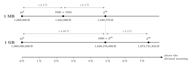
Figure 7: The three meanings of 1 MB and of 1 GB, placed on one scale by how far each lies above the decimal meaning. A binary megabyte, 1,048,576 bytes, is 4.86 per cent above a million bytes; a binary gigabyte, 1,073,741,824 bytes, is 7.37 per cent above a billion. The in-between meaning, a decimal thousand of the next binary unit down, is always one factor of 1.024 (2.4 per cent, the arrows) short of the binary one, so the in-between gigabyte lands exactly on the binary megabyte’s 4.86 per cent (dashed).
When do we use powers of 2, and when powers of 10?
- Main memory capacity is always quoted in powers of 2: \(1\text{ GB} = 1024 \times 1024 \times 1024\text{ bytes} = 2^{30}\) bytes. A memory with \(n\) address lines has exactly \(2^n\) cells (2 for one line, \(2^2 = 4\) for two, \(2^3 = 8\) for three), so memory comes in powers of 2.
- Hard disk makers quote powers of 10, \(1\text{ GB} = 1000 \times 1000 \times 1000\text{ bytes} = 10^9\) bytes, which makes a disk look bigger.
- Operating systems such as Windows count in powers of 2, which is why a new disk always shows less than its label.
- Data rates are usually powers of 10: 1 Gbps (gigabit per second) is \(10^9\) bits per second.
- Occasionally a figure mixes the two.
Worked: the 1.44 MB floppy disk
A “1.44 MB” floppy disk stores \(1.44 \times 1000 \times 1024\) bytes. How many bytes is that, and how many MB is it in each of the two pure meanings?
\[1.44 \times 1000 \times 1024 = \mathbf{1{,}474{,}560}\ \textbf{bytes}.\]
In binary megabytes that is \(1{,}474{,}560 / 2^{20} = 1.40625\) MB; in decimal megabytes, \(1{,}474{,}560 / 10^6 = 1.47456\) MB. The “1.44” is neither: it counts thousands of 1024-byte kilobytes, a decimal mega of binary kilos.
Worked: a disk in the operating system
A disk sold as 500 GB is formatted and the operating system, counting in powers of 2, reports its size. About how many “GB” does it show?
The maker’s 500 GB is \(500 \times 10^9\) bytes. The OS divides by \(2^{30}\): \(500 \times 10^9 / 1{,}073{,}741{,}824 = \mathbf{465.66}\) GB. Nothing is missing; the gigabytes differ by 7.4 %. (Formatting takes a little more, for the file system’s tables.)
Kibibytes and mebibytes
In SI units kilo, mega and giga mean powers of 10, so separate names were standardised for the binary meanings:
- 1 kibibyte \(=\) 1 KiB \(=\) 1024 bytes;
- 1 mebibyte \(=\) 1 MiB \(=\) 1024 KiB;
- 1 gibibyte \(=\) 1 GiB \(=\) 1024 MiB.
They have not caught on, and kilo, mega and giga are still used for both meanings. These notes do the same, so the context decides which is meant, and it is worth saying so when it matters.
Types of DRAM
DRAM stores bits as charge on capacitors rather than in flip-flops. Its cells are smaller, so a chip holds more bits than a static memory chip, at the cost of being slower. The cell has stayed the same while the interface has gone through many generations:
- Fast Page Mode (FPM DRAM) and Extended Data Out (EDO DRAM), a closely related pair of asynchronous designs, EDO a refinement of FPM;
- Synchronous DRAM (SDRAM), clocked, the step every later type builds on;
- Rambus DRAM (RDRAM);
- Double Data Rate DRAM (DDR DRAM), generations 1, 2, 3, 4 and now 5, which move data on both clock edges;
- and, for graphics cards, GDDR, now at GDDR7.
What each changed is in memory-technologies.
The memory hierarchy
No memory is fast, big and cheap at once, so computers use a hierarchy of them, with the CPU at the top.
| Level | Technology | Capacity | Cost per bit | Access time |
|---|---|---|---|---|
| Registers (r0 to r31 on the AVR) | flip-flops | under a kB | $$$ | ~1 ns |
| Cache, itself in levels L1, L2, L3 | SRAM | ~MB | $$ | ~10 ns |
| Main memory | DRAM | ~GB | $ | up to ~1 µs |
| Magnetic disk | HDD, or an SSD | ~TB | a fraction of a $ | ~1 to 10 ms |
| Tape, optical disk | ~PB | a smaller fraction | ~100 ms and up |
Going down the hierarchy, capacity increases, cost per bit falls, and access time grows. The values are orders of magnitude, and the point is the trend. The hierarchy is drawn as a pyramid, with the CPU at its apex, in memory-hierarchy-and-cache.
Cache memory
A CPU runs faster than its main memory can answer, and memory fast enough to keep up is too expensive to use for all of it. A CPU that waited on main memory for every access would spend most of its time idle.
A cache gets around this with a small amount of very fast memory in front of the large, slow one. It holds copies of the words in most frequent use. The CPU looks in the cache first and goes to main memory only if the word is not there, so when most accesses find their word in the cache, the average access time comes down close to the cache’s own.
Worked: why a loop runs from the cache
A program runs
for (i = 0; i < 1000; i++) { ... }, readingionce per iteration. The cache answers in 10 ns, main memory in 1 µs, and the CPU looks in the cache first. What fraction of the reads ofihit the cache, and what is their average access time?
The first read of i is a miss: i is fetched from main memory over the bus and a copy is kept in the cache. Every later read finds it there. So 999 of the 1000 reads hit, \(h = 0.999\), and
\[t_{\text{avg}} = t_c + (1 - h)\,t_m = 10 + 0.001 \times 1000 = \mathbf{11\ ns},\]
against 1000 ns with no cache. A loop that ran \(10^{20}\) times would make the single miss vanish entirely. Programs reuse the same few words like this all the time, which is why a small cache answers most accesses. The general formula, and the cases \(h\) = 90, 95 and 99 %, are in memory-hierarchy-and-cache.
Cache levels
A cache is often built in levels, each larger and a little slower than the one before. L1 is inside the CPU itself and runs at the CPU’s speed; it is small, typically 32 kB to 128 kB. L2 is bigger, typically 256 kB to 16 MB, and may be slightly slower than the CPU; it can be on the CPU’s own chip or on a separate chip, possibly in the same module. Some machines add an L3, typically 2 MB to 256 MB. The CPU tries L1, then L2, then L3, and only then main memory. These sizes are in bytes: B is a byte and b is a bit, so 32 kB is \(32 \times 1024 \times 8 = 262{,}144\) bits.
Magnetic disks
A hard disk drive (HDD) is a stack of platters with a magnetised coating, spinning together on one spindle at thousands of rpm, 10,000 rpm on a fast disk. Data is stored magnetically in circular tracks: a patch magnetised one way (north up) is a 1 and the other way (south up) a 0. The read/write heads float a few nanometres (of the order of 5 nm) above the surfaces, and both sides of each platter are usually used.
The simplified view
A disk with four platters has eight surfaces, numbered 0 to 7 from the bottom, and one read/write head per surface. The heads are on one arm assembly and move in and out together. The disk is drawn from the side, with the cylinder the heads sit over, in magnetic-disks.
Sectors, tracks and cylinders
A track is one circle on one surface, and each track is divided into sectors. A cylinder is the set of tracks at a given radial position. Assuming both sides of every platter are used,
\[\text{number of tracks in a cylinder} = 2 \times \text{number of platters},\]
so the four-platter disk has 8 tracks per cylinder. The heads move together, to a certain cylinder (magnetic-disks).
Sectors
Each track is cut into fixed-length sectors, and the sector is the smallest unit the disk handles: it always reads or writes a whole one. A sector starts with a preamble, a known pattern the head uses to synchronise to the data; then comes the data; then error correction codes (ECCs) to repair small read errors; and then an inter-sector gap before the next sector.
Laid along the track, that is PRE | DATA | ECC | GAP. It is the same pattern as a UART frame of start bit, data, parity and stop bits (serial-communication): something to synchronise on, the payload, a check, and a separator. The layout is drawn in magnetic-disks.
Worked: how much of a disk holds files
About 85 % of a disk’s capacity is usable by the operating system, and about 95 % of that is usable for user data; the remaining ~5 % is file-system overhead. What fraction of the raw capacity holds user data, and how much of a 1 TB (\(10^{12}\) byte) disk is that?
User data gets \(0.85 \times 0.95 = 0.8075\), about 81 % of the raw capacity; file-system overhead is \(0.85 \times 0.05 = 4.25\,\%\) of it. On a 1 TB disk: \(0.85 \times 10^{12} = 850\) GB for the OS, and \(0.8075 \times 10^{12} = \mathbf{807.5}\) GB for files, which an OS counting in powers of 2 shows as \(807.5 \times 10^9 / 2^{30} = 752.04\) GB.
Access time
\[\text{access time} = \text{seek time} + \text{rotational latency} + \text{transfer time}\]
The seek time is spent moving the heads to the right cylinder. The rotational latency is spent waiting for the sector to come round under the head. The transfer time is the sector passing under the head as it is read, and it is so short compared with the other two that it can be neglected.
Average seek time. Suppose seek time is proportional to the distance the heads move. Measure positions from 0 at one edge to 1 at the other, and take the start \(x\) and the target \(y\) as independent and uniformly random. The average distance is
\[\int_0^1\!\!\int_0^1 |x - y|\,dx\,dy = 2\int_0^1\!\!\int_0^x (x-y)\,dy\,dx = 2\int_0^1 \frac{x^2}{2}\,dx = \frac13,\]
so
\[\text{average seek time} = \frac13\,[\text{edge-to-edge seek time}].\]
Average rotational latency. With rotation period \(T\), the wait is anything from 0 (the sector is just arriving) to \(T\) (it has just gone by), all equally likely, so the average is
\[\text{average rotational latency} = \frac{T + 0}{2} = \frac12\,T.\]
Both are derived in more detail in magnetic-disks.
Worked: average access time of a 7200 rpm disk
What is the average access time for a hard disk which rotates at 7200 rpm and has an edge-to-edge seek time of 10 ms? (Assume that seek time is proportional to the number of tracks to seek.)
The rotation period.
\[\frac{7200}{60}\ \text{rps} = 120\ \text{rps} \quad\Rightarrow\quad T = \frac{1}{120}\ \text{s} = \frac{1000}{120}\ \text{ms} = 8.33\ \text{ms}.\]
The average access time.
\[\text{average access time} = \frac13\,[10\ \text{ms}] + \frac12\left[\frac{1000}{120}\ \text{ms}\right] + \text{negligible} = 3.33 + 4.17 \approx \mathbf{7.5\ ms}.\]
Which seek convention. This uses one third of the edge-to-edge seek, because the seek is proportional to distance and both the start and the target are random, which makes the average distance a third of the way across. Taking half instead would give \(5 + 4.17 = 9.17\) ms; half is the average only when every seek starts from an edge.
Checking “negligible”. A track holds hundreds of sectors. With 1000 sectors on the track, one passes under the head in \(8.33\ \text{ms}/1000 = 8.3\ \mu\text{s}\), about 0.1 % of the 7.5 ms.
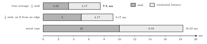
Figure 8: Three access times for the same 7200 rpm disk with a 10 ms edge-to-edge seek, drawn to scale, each a seek (dark) followed by a rotational wait (light). The true average, with both ends of the seek random, is a third of the edge-to-edge seek plus half a turn: 3.33 + 4.17 = 7.5 ms. Taking half the edge-to-edge seek, which is right only if every seek starts at an edge, overstates it at 9.17 ms. The worst case, a seek right across the disk that arrives just after the sector has passed and so waits a whole turn, is 10 + 8.33 = 18.33 ms, more than twice the average. The transfer takes microseconds and is too short to draw.
Virtual I/O: files
A program that wants to save some data should not have to know which drive, head, cylinder and sector it will land on, or what to do when a read times out and has to be retried. The operating system hides all of that behind the file, the abstraction almost all I/O goes through. To the OS a file is just a sequence of bytes; whatever structure it has, lines of text or the header of an image, is the application’s business (file-systems).
File systems
Files are far easier to use, and to program with, when they have names. A file system provides the names: it ties each file, which is really a collection of sectors, to a name in a directory. To do that it sets some sectors aside for its own index information, the File Allocation Table of the FAT file systems being one example, and uses the rest to store the files themselves. There are many file systems, differing in how they organise those tables: FAT, FAT32, exFAT, NTFS, EXT2, EXT3, EXT4, APFS, HFS+, UFS and ZFS among them.
Disk formatting
Formatting happens at two levels. A low-level format rewrites every sector from scratch, its preamble, empty data and ECC, and leaves no file system at all. A high-level format creates an empty file system by writing only the index and table sectors; the data sectors are not touched.
Deleting works the same way as a high-level format, on a smaller scale. The OS removes the file’s index entry and marks its blocks free, but it does not overwrite the sectors that hold the data. The file’s bytes are still there until something new is written over them, which is why deleted files can often be recovered (file-systems).
Files and blocks
Thanks to the OS, a file is called FinalReport.doc rather than by its cylinder and sector numbers. A program writes and reads the file as bytes; the OS keeps a map from the name to the file’s blocks, and from each block to its sectors, with the names arranged in a hierarchy of directories (folders).
Space is handed out in blocks, also called allocation units: one sector, or several consecutive sectors, typically 512 bytes to 32 kB. The block size is a trade-off. Larger blocks mean fewer of them, so a smaller map, but more space wasted at the end of each file (the EOF).
Block size and wasted space
A file fills whole blocks except the last, which is usually only partly used. The rest of that block is wasted. If the amount spilling into the last block is equally likely to be anything up to a full block,
\[\text{wasted space} \approx \frac12\,[\text{block size}]\]
per file, on average. Small blocks cut the file into many pieces with little waste at the end; large blocks cut it into few pieces with a big remainder (file-systems).
Worked: one file, three block sizes
A 10,000-byte file
test.cis stored with 512-byte, 4 kB (4096-byte) or 32 kB (32,768-byte) blocks. How many blocks does it take, and how much space is wasted? With half a block wasted per file on average, how much is wasted over 10,000 files?
The number of blocks is the size divided by the block size, rounded up.
| Block size | Blocks | Space used | Wasted at EOF | Average waste, 10,000 files |
|---|---|---|---|---|
| 512 B | \(\lceil 10000/512 \rceil = 20\) | 10,240 B | 240 B | \(10^4 \times 256 = 2{,}560{,}000\) B |
| 4096 B | \(\lceil 10000/4096 \rceil = 3\) | 12,288 B | 2,288 B | \(10^4 \times 2048 = 20{,}480{,}000\) B |
| 32,768 B | \(\lceil 10000/32768 \rceil = 1\) | 32,768 B | 22,768 B | \(10^4 \times 16384 = 163{,}840{,}000\) B |
In exchange, the map shrinks: a 1 GiB volume has \(2^{30}/512 = 2{,}097{,}152\) blocks to track at 512 B but only \(2^{30}/32768 = 32{,}768\) at 32 kB. The full comparison is in file-systems.
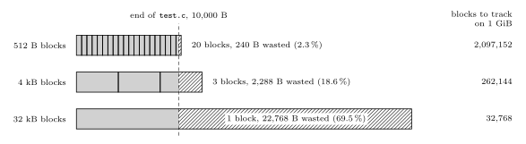
Figure 9: The 10,000-byte file test.c stored with each of the three block sizes, drawn to scale. Grey is the file and hatching the unused end of its last block; each percentage is the share of the space taken that is wasted. With 512-byte blocks the file takes 20 blocks and wastes only 240 bytes, a sliver too thin to see; with 4 kB blocks it takes 3 and wastes 2,288; with one 32 kB block it wastes 22,768 bytes, more than twice the file itself. The column on the right is the other side of the trade: the number of blocks the map must track on a 1 GiB volume falls from over two million to 32,768 as the blocks grow.
Disk allocation
Take a file of 15 sectors, with 1 block = 1 sector, on a surface of five tracks with twelve sectors each.
- (a) Contiguous: blocks 0 to 11 fill one track in order, and 12 to 14 continue on the next track. This is ideal: one seek and one rotational wait reach block 0, blocks 0 to 11 then stream past the head in a single turn, and blocks 12 to 14 cost only a step to the adjacent track and a wait for block 12 to come round.
- (b) Fragmented: the blocks are scattered over every track. That is the likely case, because disks become fragmented as files are created and deleted.
Fragmentation means slow access: each jump to another track costs a seek, and each jump to a sector that is not next under the head costs rotational latency. Both layouts are drawn on one surface in file-systems.
See also
- memory-technologies — classifying memory, SRAM and DRAM, ROM to flash, the ATmega324A’s memories, capacity units
- memory-hierarchy-and-cache — the hierarchy, cache levels, and average access time with a cache
- magnetic-disks — disk geometry, sector format, usable capacity, and the access-time derivations
- file-systems — files, formatting, deleting, block size and allocation
- memory-models · assembly-process — the ATmega324A’s address spaces and the
.cseg,.dsegand.esegsegments - 2026-10-19-floating-point-numbers — Lecture 23
Reference material
The Assembly Process
How an assembly language program becomes machine code. It covers the four fields of a statement, the directives that tell the assembler what to do as opposed to the CPU, the three memory segments of the AVR and the location counter that walks through each, and the two-pass assembler with its symbol table, which is how a program can jump to a label it has not reached yet. The program skeleton these pieces fit into is avr-program-structure, and the memories the segments map onto are in memory-models and avr-architecture. First met in 2026-10-08-assembly-process.
What an assembler does
An assembler turns a text file of assembly language into the bits that go into the chip’s memories. Most of that is translation, one statement at a time: add r1, r2 has a fixed binary form, 0000 1100 0001 0010, and nothing else in the file can change it (avr-instructions). Each instruction becomes exactly one machine instruction (instruction-set-architecture).
Two things make it more than a lookup table:
- A program is more than instructions. It has to say where things go in memory, reserve space for variables, put constant tables in flash and give registers and addresses readable names. None of that is an instruction for the CPU. These lines are directives, commands to the assembler itself.
- Names stand for numbers that are not known yet.
jmp RESETneeds the address ofRESET, and ifRESET:is further down the file, a single read from top to bottom cannot supply it. The cure is to read the file twice.
C reaches machine code by a different road: the compiler turns one line of C into many instructions (2026-09-07-introduction-to-embedded-c-programming), and how that output is joined into a program is compilation-and-linking.
The format of a statement
An assembly program is a sequence of one-line statements. A statement has up to four fields, and any of them may be empty:
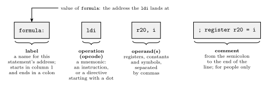
Figure 10: The four fields of one assembly statement. The label names the address this statement ends up at, so other statements can jump to it or refer to the data there. The operation field holds the mnemonic, which is either an instruction for the CPU or, if it starts with a dot, a directive for the assembler. The operands are what the operation works on: registers, constants or symbols, separated by commas. The comment runs from the semicolon to the end of the line and is thrown away by the assembler.
Label. A name for a position in memory. Labels exist so that statements can be jumped to and so that data can be referred to by name. Its value is the address the statement lands at: a word address in program memory for code, a byte address in data memory for a variable. By convention a label starts in column 1 and everything else is indented, so labels stand out down the left edge. In AVR assembly it ends with a colon.
Operation. A symbolic abbreviation for an instruction’s opcode, a mnemonic: LDS for Load Direct from data Space, ldi for load immediate. Or a directive, which starts with a dot.
Operands. The registers and addresses the instruction uses. Register names belong to the machine:
| Machine | Register names |
|---|---|
| Pentium | eax, ebx, esi, edi, … |
| SPARC | o0..o7, i0..i7, l0..l7, g0..g7 (out, in, local and global) |
| AVR | simply r0..r31 |
An address operand is usually written as a label, lds r16, count, and the assembler substitutes the number.
Comment. Space for explanation, only for people: the assembler discards it. In assembly comments are not optional politeness. ldi r20, 13 says nothing about why; the comment is the only place the intent is written down.
Ending a statement. Some assemblers want a semicolon at the end of every statement and others do not. AVR assembly does not: the end of the line ends the statement, and a semicolon starts a comment.
Directives
Besides instructions, the assembler needs other information, for example:
- where in memory the code and data should go;
- nicer names for registers and addresses, such as
tempforr16orSPHfor I/O address0x3E; - space for variables and tables of constants.
That information is given as a directive, also called a pseudo-instruction: a command to the assembler itself, written where an instruction would be and preceded by a dot, as in .byte or .def temp = r16. Most directives produce no machine code at all. They change what the assembler knows or where it is putting things.
The assembler in Microchip Studio, AVRASM2, has these, among others:
| Directive | What it does |
|---|---|
.byte |
reserve bytes for a variable |
.cseg |
switch to the code segment |
.csegsize |
set the program memory size |
.db |
define constant byte(s) |
.def |
give a register a symbolic name |
.device |
name the exact processor the program is for |
.dseg |
switch to the data segment |
.dw |
define constant word(s) |
.equ |
set a symbol equal to an expression, permanently |
.eseg |
switch to the EEPROM segment |
.exit |
stop processing this file |
.include |
read source from another file, here |
.list, .nolist |
turn generation of the list file on, off |
.listmac |
show macro expansions in the list file |
.macro, .endm (or .endmacro) |
begin, end a macro |
.org |
set the location counter: the address of what comes next |
.set |
set a symbol equal to an expression, changeably |
.if, .else, .elif, .endif |
conditional assembly: include lines only if a condition holds |
All of this is AVRASM2’s syntax. Other assemblers, even ones for the AVR, spell things differently. The GNU assembler used behind avr-gcc has a .byte directive too, and there it stores the bytes listed instead of reserving space.
Segments and location counters
The AVR has three memories (avr-architecture), and to the assembler each is a segment. Directives choose which segment the following lines go into:
| Segment | Directive | Memory | What can go there |
|---|---|---|---|
| code | .cseg |
flash, program memory | instructions, and constant data |
| data | .dseg |
SRAM, data memory | space only, reserved for variables |
| EEPROM | .eseg |
EEPROM | constants |
The data segment cannot be given values. The assembler’s output is programmed into flash and EEPROM, which keep their contents with the power off. SRAM is empty at power-up and holds nothing until the running program writes to it, so all the assembler can do there is decide which addresses each variable will use.
Each segment has its own location counter: the address the next thing in that segment will be placed at. A label takes the current value of its segment’s counter, and every statement that places something advances the counter by its size. Switching segment does not reset anything. It only changes which counter is in use, so a segment can be built up in pieces, and each piece carries on where the last piece of the same segment stopped.
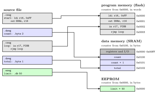
Figure 11: One source file feeding three memories. The file switches segment four times, and each piece goes to the memory its directive names, carrying on from where the previous piece of the same segment stopped: the second code piece follows the first in flash, and total follows count in SRAM. Each segment has its own location counter. The code counter starts at 0 and counts 16-bit words. The data counter starts at 0x0100, the first address after the registers and I/O, and counts bytes. The EEPROM counter starts at 0 and counts bytes. Grey marks code, blue data and green EEPROM.
Where each counter starts:
- Code: at 0, the reset address, and the assembler starts in the code segment, so a file with no segment directives is all code. The counter counts 16-bit words, because each program-memory address names a word (memory-models).
- Data: at the first free SRAM address,
0x0100on the ATmega324A, since0x0000to0x00FFare the registers and I/O registers. The counter counts bytes. - EEPROM: at 0, counting bytes.
.org sets the counter of the current segment to a given value, so whatever follows is placed there. It works in any segment, in that segment’s units.
Reserving and defining data
Three directives put data in memory:
| Directive | Segment | Places | Size |
|---|---|---|---|
.byte n |
data | nothing: reserves n bytes |
n bytes |
.db a, b, … |
code or EEPROM | constant bytes, 8 bits each | one byte each |
.dw a, b, … |
code or EEPROM | constant words, 16 bits each | two bytes each |
.byte is allowed only in the data segment: it is how a variable gets an address. .db and .dw initialise constants, so they belong where constants can live: the code segment or the EEPROM segment.
.db in the code segment packs two bytes per word. Program memory is 16 bits wide, so consecutive bytes share a word, the first in the low byte and the second in the high byte. A .db line with an odd number of bytes leaves half a word over, and the assembler fills it with a zero pad byte so that the next line starts on a whole word. Each .db line is padded on its own, so two 5-byte lines take 3 words each, not 5 words between them. AVRASM2 warns when it pads. Writing the 0 yourself gives the same layout without the warning.
.dw takes one whole word per value, so it is the natural way to store numbers bigger than 255, or addresses.
Worked: a lookup table in flash
A lookup table (LUT) is a table of constants a program reads instead of computing. Lay out:
        .cseg
table1: .db  11, 12, 30
table2: .dw  100, 133
        .org 500
table3: .dw  ...
The code counter starts at 0.
table1= 0. Three bytes: 11 and 12 share word 0, 30 takes the low half of word 1, and a pad 0 fills its high half. The counter moves to 2.table2= 2. Two words, 100 at word 2 and 133 at word 3. The counter moves to 4..org 500sets the counter to 500. Words 4 to 499 are skipped, and nothing is placed there.table3= 500 (0x01F4).
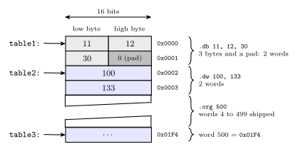
Figure 12: The lookup table laid out in program memory, one 16-bit word per row, lowest address at the top. A .db puts two bytes in each word, the first in the low byte, and pads an odd count with a zero byte so that the next label starts on a whole word: here 30 shares word 1 with a pad. Each .dw value fills a whole word. The .org moves the location counter forward and leaves words 4 to 499 untouched, so table3 lands at word 500. The diagonal break means the gap is not drawn to scale. Grey marks the .db bytes, dark grey the pad and blue the .dw words.
On the data side, two .byte 2 lines in separate .dseg pieces end up next to each other, at 0x0100 and 0x0102, whatever code sits between them in the file. That is worked in 2026-10-08-assembly-process.
Naming things: .def, .equ and .set
Three directives give a name to something. None of them places anything or moves a location counter.
| Directive | Names | Can it be changed later? | Example |
|---|---|---|---|
.def |
a register, and only a register | yes, by another .def |
.def ZH = r31 |
.equ |
a value: a number, an I/O address, an expression | no | .equ sreg = 0x3f ; Status register |
.set |
a value | yes, by another .set |
.set io_offset = 0x23 ; For now |
.equ is the usual choice for a constant, because a second definition is an error and catches a clash of names. .set is for a value that a later part of the file deliberately redefines, which is what for now in the comment above says.
Check. The same program defines .equ SPH = $3E and .def ZH = r31. Why .equ for one and .def for the other? SPH is an I/O register, which instructions such as out reach by its I/O address, 0x3E. To the assembler that is just a number, so .equ. ZH is general-purpose register r31, the high byte of the Z pointer, which instructions name as a register operand, so .def.
Two more directives are about files and the processor rather than names:
.include "file"reads another file in at that point, as if its text were typed there..include "m324Adef.inc"is howPORTA,SPH,RAMENDand the rest get defined: the file is mostly.equand.deflines (avr-io-ports)..device ATmega324Anames the exact processor. The assembler then rejects any instruction that chip does not implement..exitstops reading the file at that line. Anything after it is ignored.
The forward reference problem
Read top to bottom, most statements can be translated on the spot. add r1, r2 names two registers and nothing else, so its machine word is known at once.
A label used before it is defined is different. A program usually starts with
        jmp  RESET
        ...
RESET:  ldi  temp, low(RAMEND)
When the assembler reaches the jmp, it knows the opcode but not the operand: RESET has not been seen, so there is no address to put in the instruction. This is the forward reference problem. One forward reference anywhere in a file is enough to stop a single top-to-bottom pass from finishing the job.
The two-pass assembler
The fix is to process the file twice.
Pass one: define every symbol. Go through the file without generating anything. Keep a location counter for each segment, starting at 0 for code and EEPROM and at 0x0100 for data. For each line:
- if it has a label, enter the label in the symbol table with its segment and the current value of that segment’s counter;
- if it is
.equ,.setor.def, enter that name and its value; - if it is
.cseg,.dsegor.eseg, switch counters; if it is.org, set the current counter; - advance the current counter by the line’s size: 1 or 2 words for an instruction, the padded number of words for
.db, a word per value for.dw,nbytes for.byte n, and 0 for a line that only names something.
Pass one only needs each line’s size, and every instruction’s size is known without knowing its operands: jmp RESET takes 2 words whatever RESET turns out to be.
Pass two: assemble. Go through the file again with the counters reset. Now every symbol’s value is in the table, so each instruction can be assembled, turned into actual machine code, with its operands filled in, and each .db and .dw value can be written.
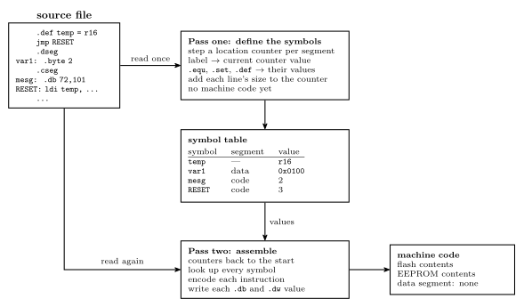
Figure 13: The two-pass assembler. Pass one reads the whole source and produces no code: it steps the location counters and records each symbol’s segment and value in the symbol table. Pass two reads the same source again from the top and, with every value now in the table, encodes each instruction and writes each constant. Its output is the contents of flash and of EEPROM. The data segment produces no output, only the addresses its labels were given.
Worked: a two-pass trace
The program:
        .equ    RAMEND = $08FF
        .equ    SPH = $3E
        .equ    SPL = $3D
        .def    ZH = r31
        .def    ZL = r30
        jmp     RESET
        .dseg
var1:   .byte   2
var2:   .byte   2
        .cseg
        .def    temp = r16
mesg:   .db     72,101,108,108,111
table:  .dw     var1, var2
RESET:  ldi     temp, low(RAMEND)
        out     SPL, temp
        ldi     temp, high(RAMEND)
        out     SPH, temp
        ...
        ldi     ZH, high(mesg*2)
        ldi     ZL, low(mesg*2)
        lpm                     ;R0 <= M[Z]
Pass one. The code counter starts at 0 and the data counter at 0x0100 (256).
- The five
.equand.deflines enterRAMEND,SPH,SPL,ZHandZLin the table and place nothing. jmp RESETis a 2-word instruction, so it takes words 0 and 1 and the code counter goes to 2.RESETis not known yet, and pass one does not need it to be..dsegswitches to the data counter.var1= 256 (0x0100) and.byte 2moves the counter to 258.var2= 258 (0x0102) and the counter goes to 260..csegswitches back to the code counter, still at 2..def temp = r16enterstemp.mesg= 2. Five bytes need three words with a pad, words 2 to 4, and the counter goes to 5.table= 5. Two words, 5 and 6, and the counter goes to 7.RESET= 7. Each of the four instructions from here is one word:ldiat 7,outat 8,ldiat 9,outat 10.
The counters run code 0, 2, 5, 7, 8, 9, 10, 11 and data 256, 258, 260. The EEPROM counter is never used.
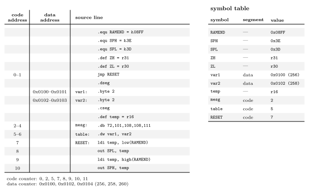
Figure 14: Pass one over the example, line by line. The two address columns show where each line is placed in its own segment, so a range means the line takes several words or bytes: the jmp two words, the 5-byte .db three words with its pad, the .dw two words, each .byte 2 two bytes. Lines that only name something or switch segment take no space and have no address. The code and data counters advance independently, which is why mesg comes straight after the jmp even though the data lines sit between them in the file. On the right is the symbol table pass one leaves behind: every name, the segment its value belongs to, and the value. The .equ and .def names have no segment.
So the instruction at RESET is at program address 7, mesg is at 2, table at 5, and the variables at 256 and 258.
Only one reference in the program is forward: jmp RESET. Every other symbol (RAMEND, var1, var2, mesg, SPL, SPH, ZH, ZL, temp) is defined above the line that uses it. One is enough to need the second pass.
Worked: what pass two writes
With the table complete, pass two replaces every symbol by its value and encodes:
| Address | Statement | With symbols replaced | Machine word(s) |
|---|---|---|---|
| 0–1 | jmp RESET |
jmp 7 |
0x940C 0x0007 |
| 2–4 | .db 72,101,108,108,111 |
bytes 72, 101, 108, 108, 111 and a pad 0 | 0x6548 0x6C6C 0x006F |
| 5–6 | .dw var1, var2 |
.dw 0x0100, 0x0102 |
0x0100 0x0102 |
| 7 | ldi temp, low(RAMEND) |
ldi r16, 0xFF |
0xEF0F |
| 8 | out SPL, temp |
out 0x3D, r16 |
0xBF0D |
| 9 | ldi temp, high(RAMEND) |
ldi r16, 0x08 |
0xE008 |
| 10 | out SPH, temp |
out 0x3E, r16 |
0xBF0E |
| later | ldi ZH, high(mesg*2) |
ldi r31, 0x00 |
0xE0F0 |
| later | ldi ZL, low(mesg*2) |
ldi r30, 0x04 |
0xE0E4 |
| later | lpm |
lpm |
0x95C8 |
Points worth checking by hand:
ldi r16, 0xFF. The form is1110 KKKK dddd KKKK, withddddthe register number minus 16.K=1111 1111anddddd=0000, so1110 1111 0000 1111=0xEF0F.- The
.dbwords. The first byte of each pair is the low byte: 72 and 101 make0x6548. The odd fifth byte, 111 =0x6F, shares its word with the pad. low()andhigh()split a 16-bit value into its bytes at assembly time.RAMEND=0x08FFgives0xFFand0x08: this is the stack pointer being set to the top of SRAM (procedures-and-the-stack).mesg*2.mesgis a word address, 2.lpmreads one byte of program memory from the byte address in Z, and word 2 starts at byte 4. So Z =0x0004, andlpmloadsr0with the byte there, 72, theHofHello. The two kinds of address are drawn in memory-models.tableholds the two variables’ addresses,0x0100and0x0102: a table of pointers, in flash, into the data segment.
Common mistakes
- Counting
jmpas one word. It is two, because it carries a full program address (avr-branches-and-jumps).rjmpis one. - Forgetting the pad. A
.dbline with an odd number of bytes takes a whole extra word, and each line is padded separately. - Counting
.dbbytes as words. Two bytes share a word in program memory. - Letting
.dseglines move the code counter, or the other way round. Each segment has its own counter, and switching segments only chooses which one is in use. - Giving size to lines that only name things.
.equ,.set,.def,.cseg,.dseg,.includeand comments place nothing. - Expecting
.byteto store a value..byte 2reserves two bytes. It does not put a 2 anywhere. Constants go in flash or EEPROM with.dbor.dw. .deffor a constant, or.equfor a register..defis for registers only.- Redefining an
.equ. It cannot be changed; that is what.setis for. - Handing a code label straight to
lpm. A code label is a word address.lpmwants the byte address, the label times 2. - Ending statements with a semicolon out of habit from another language. In AVR assembly it starts a comment.
- Assuming another assembler reads the same way. Directive names and meanings change between assemblers, even for the same chip.
See also
- avr-program-structure — the skeleton: vector table,
RESET, the main loop, and where segments and directives go in it - memory-models — word and byte addresses, cell sizes, and the AVR’s separate address spaces
- avr-architecture — flash, SRAM and EEPROM, the three memories behind the three segments · memory-technologies — what each of the three is as a technology
- avr-instructions · avr-branches-and-jumps — instruction sizes, which decide how far the code counter moves
- avr-interrupts —
.orgplacing eachjmpin the vector table - procedures-and-the-stack — the stack pointer set-up the worked example starts with
- instruction-set-architecture — assembly as a level, one line to one instruction
- compilation-and-linking — the road to machine code from C
- 2026-10-08-assembly-process — Lecture 20
Binary Number Representations
Bits, bytes, and words
- Bit = binary digit (0 or 1).
- Nibble = 4 bits. It is the unit that makes hexadecimal convenient (one hex digit = one nibble).
- Byte = 8 bits, e.g.
01010111. - Modern computers deal with words, usually a power-of-2 number of bytes: 1, 2, 4, or 8 bytes = 8, 16, 32, 64 bits. The AVR used in this course is at the small end — an 8-bit (1-byte) word; modern CPUs sit at the other end, 32- or 64-bit.
Representing whole (unsigned) numbers
Each bit position has a value — a power of 2, increasing from right (least significant) to left (most significant). Binary → decimal: add the values of each position where the bit is 1.
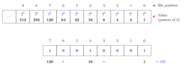
Figure 15: Place values for an unsigned binary number, and a worked conversion. Position \(i\) is worth \(2^i\), so reading a binary number is just adding the place values of the positions holding a 1: \(10010001_2 = 128 + 16 + 1 = 145\).
Most and least significant bits
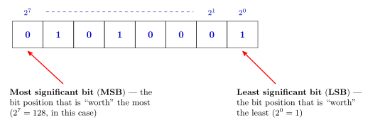
Figure 16: The two ends of a word get names, because almost every later convention (shifting, sign bits, bit numbering in AVR registers) is stated in terms of them. For an \(n\)-bit unsigned word the MSB is worth \(2^{n-1}\) — here \(2^7 = 128\) — and the LSB is always worth \(2^0 = 1\).
Converting decimal to binary
Two equivalent methods, both worked on the same number, 53.
Method 1 — sum of powers of 2. Rewrite \(n\) as a sum of powers of 2, by repeatedly subtracting the largest power of 2 not greater than \(n\) (\(53 - 32 = 21\), \(21 - 16 = 5\), \(5 - 4 = 1\), \(1 - 1 = 0\)). Then assemble the binary number from 1’s in the bit positions corresponding to those powers of 2, and 0’s everywhere else.
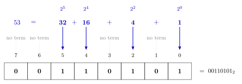
Figure 17: Method 1 on \(53\). Each power of two in the decomposition names one bit position — \(2^5\) is position 5, \(2^4\) is position 4, and so on — and every position with no term in the sum gets a 0. Reading the row off left to right gives \(00110101_2\).
Method 2 — repeated division. Build the bits up from the right (least significant): divide \(n\) by 2, the remainder (0 or 1) is the next bit, then repeat with \(n\) = the quotient. Stop when the quotient reaches 0, and read the remainders upwards.
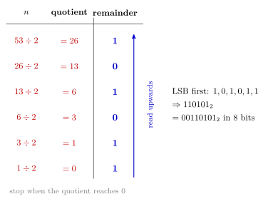
Figure 18: Method 2 on \(53\). The remainders come out LSB-first, which is why the answer has to be read back up the column: \(110101_2\), or \(00110101_2\) padded to a byte. The same procedure with a divisor of 16 or 8 converts to hexadecimal or octal instead.
Number range (unsigned)
- Smallest representable value: all 0’s → 0.
- Largest representable value: all 1’s → for an \(n\)-bit word, \(2^n - 1\) (e.g. 255 for 8 bits).
The \(-1\) is the part worth understanding: an \(n\)-bit word has \(2^n\) distinct patterns, but one of them is spent on zero.
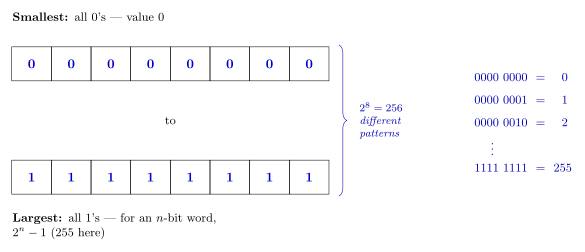
Figure 19: Why the largest unsigned value is \(2^n-1\) and not \(2^n\). Counting up from all-zeros steps through every pattern in turn — each extra bit doubles how many there are, so 8 bits give \(2^8 = 256\) patterns — and because the count starts at 0, the last one is 255.
Other radices
Radix = number system base. A radix-\(k\) number system has \(k\) distinct symbols for digits \(0\) to \(k-1\), and the value of each digit (from the right) is \(k^0, k^1, k^2, \dots\) — so a radix-\(k\) number \(d_{m}\dots d_1 d_0\) is worth \(\sum_i d_i k^i\). E.g. \(1\mathrm{A}_{16} = 1 \cdot 16^1 + 10 \cdot 16^0 = 16 + 10 = 26\).
- Octal (radix-8): symbols
0–7. One octal digit corresponds to exactly 3 bits. - Hexadecimal (radix-16): symbols
0–9,A–F. One hex digit corresponds to exactly 4 bits — very convenient for grouping binary.
| Dec | 0 | 1 | 2 | 3 | 4 | 5 | 6 | 7 | 8 | 9 | 10 | 11 | 12 | 13 | 14 | 15 | 16 | 17 |
|---|---|---|---|---|---|---|---|---|---|---|---|---|---|---|---|---|---|---|
| Oct | 0 | 1 | 2 | 3 | 4 | 5 | 6 | 7 | 10 | 11 | 12 | 13 | 14 | 15 | 16 | 17 | 20 | 21 |
| Hex | 0 | 1 | 2 | 3 | 4 | 5 | 6 | 7 | 8 | 9 | A | B | C | D | E | F | 10 | 11 |
Converting binary ↔︎ hex/octal by grouping
Because \(16 = 2^4\) and \(8 = 2^3\), no arithmetic is needed: group the bits from the right — four at a time for hex, three at a time for octal — and translate each group with the table above. Pad the leftmost group with leading zeros.
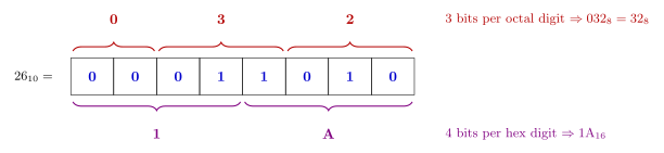
Figure 20: One bit pattern read two ways. Grouping \(00011010_2\) into nibbles from the right gives \(1\) and \(\mathrm{A}\), i.e. \(1\mathrm{A}_{16}\); grouping the same bits in threes gives \(0\), \(3\) and \(2\), i.e. \(32_{8}\). The grouping must start at the right — starting at the left gives the wrong answer whenever the width is not a multiple of 3 or 4.
The same trick read backwards is why hex is used for bit patterns at all: a full byte of 1’s, 1111 1111, is F F = \(\mathtt{0xFF}\) = 255, and any byte can be written as two hex digits.
To convert decimal → any radix, use Method 2 with that radix as the divisor: \(26 \div 16\) gives quotient 1 remainder 10 (= A), so \(26_{10} = 1\mathrm{A}_{16}\); \(26 \div 8\) gives quotient 3 remainder 2, so \(26_{10} = 32_8\). See 2026-07-27-course-intro-bits-bytes-binary for that worked exercise.
Radix notation conventions
Since a bare number like 101 or 747 is ambiguous, a radix indicator is needed. A subscript works generically (e.g. \(101_2\), \(101_{16}\)); in code/assembly, conventions vary. Bolded rows are the ones this course mostly uses:
| Radix | Convention | Example | Where used |
|---|---|---|---|
| any | subscript | \(101_2\), \(101_{16}\) | generic/mathematical |
| Hex | leading 0x |
0x101 |
C, Atmel AVR |
| Hex | trailing h |
101h |
some assembly languages |
| Hex | leading $ |
$747 |
Atmel AVR assembly |
| Octal | leading 0 |
0101 |
C, Atmel AVR |
| Octal | trailing q |
101q |
some assembly languages |
| Octal | leading @ |
@747 |
some assembly languages |
| Binary | leading 0b |
0b101 |
Atmel AVR assembly, some C |
| Binary | trailing b |
101b |
some assembly languages |
| Binary | leading % |
%101 |
some assembly languages |
The octal convention is the trap: in C, a leading 0 silently changes the radix, so 0101 is \(65_{10}\), not \(101_{10}\).
Representing signed numbers
Computers don’t store \(+\) and \(-\) signs; the sign has to be encoded in the bits themselves. Four formats have been used, and all four — plus unsigned — represent positive numbers identically. Only the negatives differ.
Signed magnitude
The leftmost bit is a sign bit (0 positive, 1 negative) and contributes nothing to the magnitude. Negate by inverting the sign bit alone.
Ones’ complement
The sign bit now also carries weight: its position value is \(-(2^{N-1}-1)\). Negate by inverting all the bits.
Two’s complement
The sign bit’s position value is \(-2^{N-1}\). Negate by inverting all the bits and adding 1. This is the one actually used in practice.
Compare the position values, 8-bit:
| bit 7 | 6 | 5 | 4 | 3 | 2 | 1 | 0 | |
|---|---|---|---|---|---|---|---|---|
| Signed magnitude | sign | 64 | 32 | 16 | 8 | 4 | 2 | 1 |
| Ones’ complement | \(-127\) | 64 | 32 | 16 | 8 | 4 | 2 | 1 |
| Two’s complement | \(-128\) | 64 | 32 | 16 | 8 | 4 | 2 | 1 |
Excess-\(2^{N-1}\)
For 8 bits, “excess 128”: the value stored is the true value plus 128. So \(-3\) is stored as \(125\) and \(3\) as \(131\).
It is exactly two’s complement with the sign bit reversed — a 0 in the MSB means bit value \(-128\), a 1 means 0. Its practical use is that comparing two signed numbers becomes simple in hardware. The exponent of an IEEE floating-point number is stored in excess notation for exactly that reason, with a bias one smaller: excess-127 for 8 bits (floating-point-numbers).
Ranges
| Format | 8-bit | \(n\)-bit |
|---|---|---|
| Unsigned | \(0\) to \(255\) | \(0\) to \(2^n - 1\) |
| Signed magnitude | \(-127\) to \(127\) | \(-(2^{n-1}-1)\) to \(2^{n-1}-1\) |
| Ones’ complement | \(-127\) to \(127\) | \(-(2^{n-1}-1)\) to \(2^{n-1}-1\) |
| Two’s complement | \(-128\) to \(127\) | \(-2^{n-1}\) to \(2^{n-1}-1\) |
| Excess-\(2^{n-1}\) | \(-128\) to \(127\) | \(-2^{n-1}\) to \(2^{n-1}-1\) |
Worked example — \(\pm 47\) in 8 bits
\(+47 = \texttt{00101111}\) in every format.
| Format | \(-47\) | How |
|---|---|---|
| Signed magnitude | 10101111 |
flip the sign bit |
| Ones’ complement | 11010000 |
invert all bits |
| Two’s complement | 11010001 |
invert all bits, add 1 |
| Excess-128 | 01010001 |
\(-47 + 128 = 81\) |
And in 4 bits, \(-3\) is 1100 in ones’ complement and 1101 in two’s complement.
Why “complement”?
A thing and its complement together make a whole — an angle and its complement make a right angle, a set and its complement a universal set.
- Ones’ complement: a number plus its negative gives a string of ones (
11111111in 8 bits). - Two’s complement: a number plus its negative gives a power of two, with overflow (
1 00000000). It would more accurately be called power-of-two’s complement.
Base 10 has the same pair — nines’ and ten’s complement — used on early mechanical adding machines to do subtraction.
Why two’s complement wins
Two representations of zero, which wastes a bit pattern that could have extended the range:
- Signed magnitude:
00000000and10000000 - Ones’ complement:
00000000and11111111
Asymmetric range: two’s complement and excess-\(2^{n-1}\) (one more negative than positive).
Arithmetic: signed-magnitude addition requires taking cases; ones’ complement addition requires an extra addition step (the end-around carry); sign extension and comparison are non-trivial in both. Two’s complement has a single zero and its addition is just binary addition — no special cases.
Format matters
The same eight bits mean different things under different formats. 10010010 reads as:
| Read as | Value |
|---|---|
| Unsigned | 146 |
| Two’s complement | \(-110\) |
| Ones’ complement | \(-109\) |
| Signed magnitude | \(-18\) |
| Excess-128 | 18 |
Or 01010101: 85 unsigned, \(-43\) in excess-128, 'U' in ASCII, or 10.625 as fixed point with 5 bits before the binary point and 3 after.
The format is not encoded in the data. It has to be known separately — by a human, by a program, or by the hardware. See week1-lab-number-representations for the full 4-bit table across all five formats, and 2026-08-04-binary-arithmetic for what happens when you add these.
Fractions: fixed and floating point
Everything above is whole numbers. Place values carry on past a binary point as \(\tfrac12, \tfrac14, \tfrac18, \dots\), and there are two ways to use them.
- Fixed point: agree where the point sits, as in the 5.3 reading of
01010101above, and read the bits as before. Ordinary integer hardware does the arithmetic, but the format fixes the range and the precision once and for all. See fixed-point-numbers. - Floating point: store the digits and the position of the point separately, as binary scientific notation: a sign, a biased exponent and a mantissa. This is IEEE 754, the
floatanddoubleof C. See floating-point-numbers.
C Language Basics
What a C program is made of: the shape of a program, variables and their types, functions, and constants. Operators are in c-operators, the if/while/for statements in c-control-flow, arrays and pointers in c-pointers-and-arrays, and the preprocessor in c-preprocessor-and-avr-headers. First met in 2026-09-07-introduction-to-embedded-c-programming.
Where C sits
C is the top layer of the course’s three blocks — high-level programming over low-level programming over digital logic design — and the course’s C is embedded C for the ATmega324A, the same chip the assembly targeted. The difference from assembly is one extra tool. An assembler turns each line into exactly one instruction; a compiler turns each C statement into however many instructions it needs, chooses the registers, and hands the result to the assembler. The chain from C statement down to control unit is drawn in 2026-09-07-introduction-to-embedded-c-programming, and the steps after the compiler, object files and the linker, are in compilation-and-linking.
What is expected: write small C programs and functions from scratch, understand the meaning of C programs, and write or modify C programs — practised in Labs 11–16, which all use C.
The shape of a program
- There must be a function called
main; it is executed when the program starts. - Blocks of code are enclosed by braces
{ }. - Statements end with a semicolon
;. - C is case sensitive —
variableandVariableare different names. - Comments are
/* … */(any length, may span lines) or//to the end of the line.
/* the smallest useful embedded program: */
#include <avr/io.h>

int main(void) {
    DDRA = 0xFF;        /* a statement */
    while(1) {          /* a block */
        PORTA = 0x55;
    }
}
On the AVR main never returns — there is no operating system to return to — so every program ends in an infinite loop (c-control-flow). #include is the preprocessor’s (c-preprocessor-and-avr-headers).
Variables and types
Declaration: type-name variable-name, variable-name …;
A declaration reserves room in data memory (memory-models) and gives it a name and a type. The type decides two things: how many cells the variable takes, and how the bits are read — the signed/unsigned question of binary-number-representations, now answered once at the declaration instead of instruction by instruction.
| Declaration | Size | Range | |
|---|---|---|---|
char c; |
1 byte | −128 … 127 | two’s complement |
unsigned char x; |
1 byte | 0 … 255 | |
int day; |
machine dependent — 16 bits on the AVR | −32768 … 32767 | two’s complement |
unsigned int count; |
as int |
0 … 65535 on the AVR | |
float |
32 bits | about \(\pm 3.4 \times 10^{38}\), 7 digits | IEEE single precision; no AVR hardware — done in software |
double |
64 bits in general; 32 on avr-gcc | likewise |
On avr-gcc float and double are interchangeable: both are 32 bits (below).
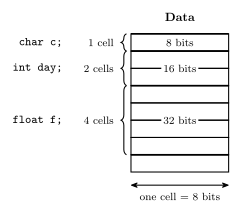
Figure 21: What three declarations reserve in the AVR’s 8-bit data memory, drawn as a memory map. char is one cell. int is two, because int is 16 bits on the AVR — which is why a pointer to an int steps by two in the pointers note. float is four, because single precision is 32 bits. The compiler decides the actual addresses; the addresses here are schematic and the order is arbitrary.
Three consequences worth carrying around:
charis an integer. It is exactly the 8-bit two’s complement byte of the hardware block; the name only promises it can hold a character code. Arithmetic on it is byte arithmetic, and'A' + 1is'B'because'A'is 65.intis not one size. Write code that assumes 16 bits and it breaks on a desktop; assume 32 and it breaks on the AVR. The AVR headers provideuint8_t,int16_tand friends — types with the width in the name — and the course’s example program usesuint8_tfor exactly this reason.- Nothing is checked. Storing 300 in an
unsigned chardoes not fail; it stores 300 mod 256, i.e. 44. (For a signedcharthe C standard leaves the result implementation-defined; gcc also gives 44.) The type is a reading rule, not a guard.
Booleans. There is no boolean type in the course’s C. Any value can be treated as a boolean: zero means false, non-zero means true. This is what lets if(a) mean if(a != 0) (c-control-flow).
Functions
return-type function-name (arg-decl)
{
    variable-declarations;
    …
    statements;
}| Part | Meaning | Example |
|---|---|---|
return-type |
what type is returned, or void for nothing |
int, void |
function-name |
the name; main for the entry point |
average |
arg-decl |
argument (parameter) declarations, comma-separated, each with its type | int a, float b |
variable-declarations |
variables used only within the function | int avge; |
statements |
the code which actually does stuff |
An example:
/*
  Return the average of two integers
  (result will be rounded towards 0)
*/
int average(int a, int b) {
    int avge;

    avge = (a+b)/2;

    return avge;
}
avge = (a+b)/2;is a statement built from expressions —(a+b), then(a+b)/2, then the assignment; the outermost expression plus its semicolon is the statement.return avge;hands the value back and ends the function.avgeis local: it exists only whileaverageis running. Nothing outside can name it.- Integer division truncates toward zero.
average(1, 2)computes3/2and returns1; the.5never exists. The comment says rounded towards 0, and that is the whole of C’s rule for/on integers —-3/2is-1, not-2.
A function with void in front returns nothing and is called for its effect. int main(void) is a function whose argument list is explicitly empty.
Where a variable lives
Where a declaration is written decides where the compiler stores the variable and how long it exists.
| Declaration | Kind | Stored | Exists |
|---|---|---|---|
outside every function: int count; |
global | at a fixed address in data memory, from 0x0100 up |
for the whole run |
inside a function: int avge; |
local | in the call’s stack frame | only while that call runs |
inside a function: static int calls; |
static local |
with the globals, at a fixed address | for the whole run, keeping its value between calls |
outside every function: static int a; |
static global |
like any global | for the whole run; the name is private to its file |
So avge in average above is made fresh on every call and is gone at the return, and a local that is never assigned starts out holding whatever was left on the stack. A static local is the way to have a function remember something from one call to the next. Memory obtained from malloc() comes from a third place, the heap, which grows from above the globals toward the stack. The full picture is in compilation-and-linking, and the frame itself is in procedures-and-the-stack.
Constants
Character constants
Single quotes: 'a', 'b', '1'. A character constant is a number — its ASCII code — so '1' is 49, not 1.
| Range | Codes |
|---|---|
'A' … 'Z' |
65 … 90 |
'a' … 'z' |
97 … 122 |
'0' … '9' |
48 … 57 |
Which makes c - '0' the digit value of a digit character, and c + ('a' - 'A') the lower-case of an upper-case letter — both plain integer arithmetic.
Special characters are backslash escaped:
'\n' |
newline |
'\'' |
single quote |
'\t' |
tab |
'\\' |
backslash |
String constants
Double quotes, escapes allowed inside: "abc \n \" hello\t". A string is an array of char (c-pointers-and-arrays).
Integer constants
| Base | Written | Examples |
|---|---|---|
| Decimal | as usual | 3, -27, 65535, +5 |
| Hexadecimal | leading 0x |
0x5F, 0xFFFF, 0xDEADBEEF |
| Octal | leading 0 |
0377 = 255 |
The octal rule is a trap: a leading zero changes the base. 010 is eight. Do not zero-pad a decimal constant.
Hexadecimal is the natural notation for anything that is really a bit pattern — port values, masks — because each digit is exactly one nibble (binary-number-representations). 0xFF is 11111111 at a glance; 255 is not.
Floating point constants
Include a decimal point and/or an e exponent: 3.1416, -7., 6.02e23, -5.2e-2. 7 is an integer; 7. is floating point. The type of a constant is decided by how it is written, and it decides what arithmetic happens: 7/2 is 3, 7./2 is 3.5.
Floating point on the AVR
float and double are usually IEEE single and double precision, but the C standard only asks for minimums: about 6 significant decimal digits for float and 10 for double, both up to \(10^{37}\). avr-gcc makes double the same 32-bit single precision as float, which gives about 7 digits and so falls short of what the standard asks of double. Code written for a desktop that relies on double quietly loses half its digits on the AVR.
The AVR also has no floating-point hardware: its only hardware data type is the 8-bit integer (instruction-set-architecture). Every float add, multiply or conversion is a call into a software library, hundreds of instructions with branches where an integer operation takes a few. So where integer arithmetic can give the same result, use it:
PORTB = PINA / 3;        /* integer: a handful of instructions, no branches */
PORTB = PINA * 0.334f;   /* float: the same results, 300+ instructions      */
Scaling to whole units (millivolts, tenths of a degree) or using fixed-point-numbers keeps the fractions without the floats. The formats themselves, and why 0.1 cannot be stored exactly, are in floating-point-numbers.
See also
- c-operators · c-control-flow · c-pointers-and-arrays · c-preprocessor-and-avr-headers
- binary-number-representations — the signed/unsigned readings behind
charandunsigned char - floating-point-numbers — what
floatanddoublehold, and their cost on the AVR · fixed-point-numbers — fractions in integer arithmetic - memory-models — the 8-bit data cells a declaration reserves
- instruction-set-architecture — the data types the AVR supports in hardware, and the ones it does not
- compilation-and-linking — how the compiler maps globals, locals and statics to memory, and what happens after compiling · procedures-and-the-stack — the stack frame a local lives in
- 2026-09-07-introduction-to-embedded-c-programming — Lecture 13 · 2026-10-15-compilation-and-linking — Lecture 22 · 2026-10-19-floating-point-numbers — Lecture 23
File Systems
How an operating system turns a disk full of numbered sectors into named files. This note covers the file as the common I/O abstraction, what a file system does and the tables it keeps, low-level and high-level formatting, why deleting a file does not erase it, allocation in blocks and the trade-off in choosing a block size, and contiguous against fragmented allocation. The sectors, tracks and cylinders underneath are in magnetic-disks. First met in 2026-10-22-memory-disks-and-files.
The file: a sequence of bytes
Nobody writing a program wants to deal with drive unit numbers, heads, cylinders and sectors, or with timeout errors and retries when a read fails. The operating system hides all of that behind one abstraction, the file.
To the operating system, a file is just a sequence of bytes. It can be read from, written to and extended, and it has a current position where the next read or write happens. Any structure inside it is up to the application program: a C source file is lines of text, an image file has a header and pixel data, but the OS sees bytes in both cases. The same read and write work on all of them.
What a file system does
Computers are far easier to use, and to program, when files have names: FinalReport.doc rather than “cylinder 412, head 3, sectors 17 to 40”. A file system provides this. It associates files, which are collections of sectors, with names and directories.
To do that it divides the disk’s sectors into two kinds:
- index sectors, holding the file system’s own tables: which names exist, in which directories, and which sectors belong to each file. The File Allocation Table (FAT) of the FAT file systems is one such table;
- data sectors, which store the files themselves.
The OS maintains a map from each file name to a set of blocks (below), and each block to its sectors. To help users, names are organised in a hierarchy of directories, or folders.
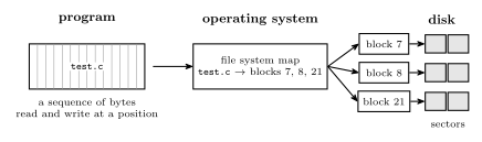
Figure 22: The layers between a program and the disk. The program reads and writes a file as a single sequence of bytes, at a current position. The operating system’s file system keeps a map from the file’s name to the blocks that hold it, and each block is one or more consecutive sectors on the disk. Neither the blocks nor the sectors need be next to one another: the map is what makes a scattered set of sectors look like one file.
There are many file systems, which differ in how they lay out their tables and what they record: FAT, FAT32, exFAT (memory cards, USB sticks), NTFS (Windows), EXT2, EXT3, EXT4 (Linux), APFS, HFS+ (macOS), UFS (BSD Unix), ZFS, and more.
Formatting
Formatting comes at two levels.
| Low-level format | High-level format | |
|---|---|---|
| What it does | reinitialises every sector: writes each one’s preamble, empty data and ECC | creates an empty file system |
| What it writes | the whole disk | only the index (table) sectors |
| File system afterwards | none | an empty one |
| Old data afterwards | gone | still in the data sectors, unreferenced |
A low-level format lays out the sector structure of magnetic-disks, so it touches every sector and takes a long time. A high-level format, what an operating system does when it is asked to “format” a disk, only writes fresh, empty tables, so it is quick, and it leaves the old files’ bytes where they were.
Deleting does not erase
Deleting a file does not mean it is gone. To delete a file, the OS may just delete its index entry and mark its blocks as free. It does not overwrite the sectors where the data is stored: that would cost a write to every sector for no benefit to the user.
The bytes stay on the disk until new files happen to be given those blocks and overwrite them. That is how undelete and data-recovery tools work, and why a disk being given away should be overwritten, not just emptied or quickly formatted.
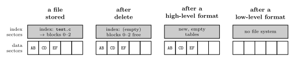
Figure 23: What deleting a file and the two kinds of format each change. The disk has index sectors, holding the file system’s tables, and data sectors, holding the files. Deleting a file removes its entry from the index and frees its blocks, but its bytes stay in the data sectors until something else is written there. A high-level format writes fresh, empty tables and leaves the data sectors alone. Only a low-level format rewrites every sector.
Blocks
File storage is allocated in blocks, also called allocation units or clusters. A block can be as small as one sector, or several consecutive sectors. Typical block sizes run from 512 bytes to 32 kB.
A file always occupies a whole number of blocks. The last block is usually only partly filled, and the rest of it is wasted: no other file can use it. So the choice of block size is a trade-off.
- Larger blocks mean fewer blocks per file, so a smaller map from names to blocks, and less work to find and read a file’s blocks; but more wasted space at the end of each file (at the EOF, end of file).
- Smaller blocks waste less at the end of each file, but the map is larger and a file is split into more pieces.
On average, a file wastes half a block. A file’s length is very unlikely to be an exact number of blocks. If the amount it spills into its last block is equally likely to be anything from nothing to a whole block, the unused part of that block is, on average,
\[\text{wasted space per file} \approx \tfrac12 \times \text{block size}.\]
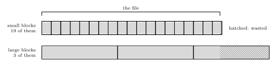
Figure 24: One file stored with small blocks and with large ones. The file’s bytes fill whole blocks until the last, which is only partly used; the rest of that block, hatched, is wasted, because no other file can use it. With small blocks the waste is small but the file needs many blocks and the map must list them all. With large blocks the map is short but the waste can approach a whole block. On average the waste is half a block per file.
Worked: choosing a block size
A 10,000-byte source file is stored on a disk formatted with 512-byte, 4 kB or 32 kB blocks (kB here meaning 1024 bytes). For each block size, how many blocks does the file take, how much space is wasted at its end, and how many blocks must the map track for a 1 GiB volume? On a disk of 10,000 files, how much space is wasted on average?
Blocks for the file is the file size divided by the block size, rounded up: a file cannot use part of a block.
| Block size | Blocks | Space taken | Wasted at the end | Waste as share of the space taken |
|---|---|---|---|---|
| 512 B | \(\lceil 10000/512 \rceil = 20\) | 10,240 B | 240 B | 2.3 % |
| 4 kB = 4096 B | \(\lceil 10000/4096 \rceil = 3\) | 12,288 B | 2,288 B | 18.6 % |
| 32 kB = 32,768 B | \(\lceil 10000/32768 \rceil = 1\) | 32,768 B | 22,768 B | 69.5 % |
Map size. A 1 GiB volume is \(2^{30}\) bytes, so it has \(2^{30}/512 = 2{,}097{,}152\) blocks of 512 B, \(2^{30}/4096 = 262{,}144\) blocks of 4 kB, and \(2^{30}/32768 = 32{,}768\) blocks of 32 kB. The map must track every one of them, so the largest blocks give a map 64 times smaller than the smallest.
Waste across the disk. At half a block per file, 10,000 files waste about
| Block size | Average waste per file | For 10,000 files |
|---|---|---|
| 512 B | 256 B | 2,560,000 B \(\approx\) 2.44 MiB |
| 4 kB | 2 kB | 20,480,000 B \(\approx\) 19.53 MiB |
| 32 kB | 16 kB | 163,840,000 B \(\approx\) 156.25 MiB |
So small blocks suit a disk of many small files, where large blocks would waste much of the space. Large blocks suit a disk of a few large files, where half a block per file is nothing and the short map and fewer pieces per file pay off.
Contiguous and fragmented allocation
Where a file’s blocks are placed on the disk decides how fast it can be read.
- Contiguous allocation puts the blocks one after another along a track, then on the next track of the same or the adjacent cylinder. Reading the file costs one seek and one rotational wait to reach its first block, after which the sectors stream past the head in order. Moving on to the next track costs only a step to the adjacent track (or none at all, if it is another surface of the same cylinder, which is just a switch of head) and a wait for the next block to come round.
- Fragmented allocation scatters the blocks over different tracks and sectors. Every jump to a different track costs a seek, and every jump to a sector that is not the next one along costs rotational latency (magnetic-disks).
Contiguous allocation is ideal, but over time it becomes unlikely: as files are created, grown and deleted, the free space breaks up into small scattered pieces, and a new file has to be put in whatever pieces are free. The disk becomes fragmented, and fragmentation makes access slow. Defragmenting moves each file’s blocks back together. (An SSD has no seek or rotation, so fragmentation costs it far less.)
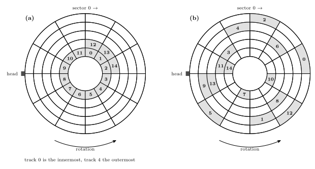
Figure 25: Two ways the same 15-block file can be stored, one block to a sector, on a surface with five tracks of twelve sectors. Sectors are numbered clockwise from the top and the disk turns so that they pass the head in that order. In (a) the blocks are contiguous: 0 to 11 fill one track in order and 12 to 14 continue on the next. One seek and one wait reach block 0, a single turn reads blocks 0 to 11, and then the head steps out to the adjacent track and waits for block 12 to come round before reading the last three. In (b) the disk is fragmented and the blocks are scattered over every track, so reading them in order needs a seek almost every time and a wait for the next block to come round.
Common mistakes
- Thinking delete or a quick format erases data. Both rewrite only the index; the bytes remain until overwritten.
- Rounding the block count down. A 10,000-byte file in 4096-byte blocks needs 3 blocks, not 2: \(\lceil 10000/4096 \rceil = 3\).
- Assuming bigger blocks are always better. They shrink the map but waste half a block per file on average, which adds up on a disk of small files.
- Confusing a block with a sector. The sector is the disk’s unit; the block is the file system’s, one or more consecutive sectors.
- Thinking the OS sees structure in a file. To the OS a file is bytes. Lines, records and headers are the application’s business.
See also
- magnetic-disks — tracks, sectors, cylinders and the access time that fragmentation inflates
- memory-hierarchy-and-cache — the disk level of the hierarchy
- memory-technologies — flash and SSDs, and the units disk sizes are quoted in
- 2026-10-22-memory-disks-and-files — Lecture 24
Fixed-Point Numbers
How a fixed number of bits can hold a fraction: put a binary point at an agreed place and give the bits to its right the weights \(\tfrac12, \tfrac14, \tfrac18, \dots\) This note covers the binary point and its place values, converting a decimal value such as 4.375 into bits, the \(m.n\) format names, reading a bit pattern in a given format, unsigned and two’s complement fixed point, and the trade-off between range and precision as the point moves across a byte. The way round that trade-off, letting the point float, is in floating-point-numbers. Whole numbers and the signed formats this builds on are in binary-number-representations. First met in 2026-10-19-floating-point-numbers.
The binary point
Binary place values carry on to the right of the point exactly as decimal ones do. In decimal the column after the point is worth \(10^{-1}\); in binary it is worth \(2^{-1} = \tfrac12\), the next \(2^{-2} = \tfrac14\), then \(\tfrac18\), \(\tfrac1{16}\), and so on, each half the one before.
| Position | \(2^3\) | \(2^2\) | \(2^1\) | \(2^0\) | . | \(2^{-1}\) | \(2^{-2}\) | \(2^{-3}\) | \(2^{-4}\) |
|---|---|---|---|---|---|---|---|---|---|
| Worth | 8 | 4 | 2 | 1 | . | 0.5 | 0.25 | 0.125 | 0.0625 |
The point is not stored anywhere. The bits are an ordinary 8-bit pattern, and where the point sits is an agreement, made by whoever writes the program, in the same way that “this byte is two’s complement” is an agreement (binary-number-representations). Because the agreed place never moves, the scheme is called fixed point.
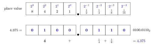
Figure 26: Eight bits with the binary point agreed to sit after the fourth. The four bits to the left are worth 8, 4, 2 and 1 as usual; the four to the right carry on halving, to 1/2, 1/4, 1/8 and 1/16. The value 4.375 is 4 + 1/4 + 1/8, so the bits worth 4, 1/4 and 1/8 are set and every other bit is 0, giving 0100.0110. Nothing in the byte marks where the point is: the same eight bits read as a whole number are 70, which is 4.375 times 16.
Converting a decimal value
Two methods, both worked on 4.375 into a format with 4 bits after the point.
Method 1: whole part and fraction separately. The whole part converts as usual: \(4 = 100_2\). The fraction converts by repeated doubling: double it, the digit before the point is the next bit, and carry on with what is after the point. Stop when the fraction reaches 0 or the bits run out.
| Fraction | \(\times 2\) | Bit | Carry on with |
|---|---|---|---|
| 0.375 | 0.75 | 0 | 0.75 |
| 0.75 | 1.5 | 1 | 0.5 |
| 0.5 | 1.0 | 1 | 0 |
The bits come out left to right, starting just after the point: \(0.375 = 0.011_2\). So \(4.375 = 100.011_2\), and padded to four bits each side, 0100.0110.
Doubling is the mirror image of the repeated division for whole numbers (binary-number-representations): division pulls bits off the right-hand end, doubling pulls them off the left-hand end of the fraction. The fraction can also be taken apart by subtraction, as with Method 1 for whole numbers: \(0.375 - 0.25 = 0.125\), and \(0.125 = \tfrac18\), so the bits worth \(\tfrac14\) and \(\tfrac18\) are set.
Method 2: scale to a whole number. With \(n\) bits after the point, every value is a whole number of \(2^{-n}\) steps. Multiply by \(2^n\), convert the whole number, and put the point back \(n\) places from the right. With \(n = 3\): \(4.375 \times 8 = 35 = 100011_2\), so \(4.375 = 100.011_2\). With \(n = 4\) it is \(4.375 \times 16 = 70 = 1000110_2\), the same bits with one more 0 on the end.
If the product is not a whole number, the value has no exact representation with \(n\) fractional bits (below).
Format names: \(m.n\)
A fixed-point format is named by how the bits are split: \(m.n\) means \(m\) integer bits before the point and \(n\) fractional bits after it, \(m + n\) bits in all. Every 8-bit format has \(m + n = 8\):
- 8.0 is an ordinary unsigned byte, the point after the last bit;
- 5.3 has five integer bits and three fractional bits,
xxxxx.xxx; - 0.8 has the point before the first bit, so every value is below 1.
The same value sits in different formats with the point in different places. \(4.375\) is 0100.0110 in 4.4, 00100.011 in 5.3, and 100.01100 in 3.5. Moving the point one place right with the bits fixed doubles the value; so to keep the value the same, the bits have to move the other way.
Reading a pattern
To find the value of a bit pattern in a given format, either add the place values of the 1 bits, or read the bits as a whole number and divide by \(2^n\). The second is quicker when the pattern is long.
10110101 as unsigned 5.3: the whole number is \(181\), and \(181 / 2^3 = 22.625\). By place values, \(10110.101_2 = 16 + 4 + 2 + \tfrac12 + \tfrac18 = 22.625\), the same.
Two’s complement fixed point
Signed fixed point uses two’s complement in the same way as signed whole numbers (binary-number-representations). The MSB’s weight is negated: in an \(m.n\) format it is worth \(-2^{m-1}\) instead of \(+2^{m-1}\), and every other bit keeps its place value. So in 5.3 the bits are worth
\[-16,\ 8,\ 4,\ 2,\ 1\ .\ \tfrac12,\ \tfrac14,\ \tfrac18\]
and in 4.4 they are worth \(-8, 4, 2, 1, \tfrac12, \tfrac14, \tfrac18, \tfrac1{16}\).
Negating works as for integers: invert every bit and add 1 at the last place, which is now worth \(2^{-n}\), not 1. Equivalently, the value is the unsigned reading minus \(2^m\) whenever the MSB is 1, which is the divide-by-\(2^n\) rule with \(256\) subtracted first: 10110101 is \((181 - 256)/8 = -75/8 = -9.375\) in two’s complement 5.3. The same question with the two tempting wrong answers, \(-10.625\) and \(-9.625\), explained is 2026-10-19-floating-point-numbers.
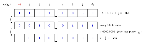
Figure 27: Two’s complement fixed point in the 4.4 format. The only change from unsigned is the MSB, whose weight becomes minus 8 instead of plus 8; the fraction bits keep their positive weights. So 1101.1000 is minus 8 plus 4 plus 1 plus 1/2, which is minus 2.5. Negating it still means inverting every bit and adding one, but the one is added in the last place, which is worth 1/16: 0010.0111 plus 0.0001 is 0010.1000, which is plus 2.5.
Range against precision
Eight bits give 256 patterns whatever the format. The format only decides how far apart the 256 values are and so how far they reach. For an unsigned \(m.n\) format:
- the precision, the gap between neighbouring values, is the weight of the last bit, \(2^{-n}\);
- the maximum is all ones, \((2^8 - 1) \times 2^{-n} = 255 \times 2^{-n}\), one step short of \(2^m\);
- the minimum is 0.
Two’s complement \(m.n\) has the same precision and runs from \(-2^{m-1}\) to \(2^{m-1} - 2^{-n}\).
| Format | Unsigned maximum | Precision | Two’s complement range |
|---|---|---|---|
| “10.$-$2” | 1020 | 4 | \(-512\) to \(508\) |
| “9.$-$1” | 510 | 2 | \(-256\) to \(254\) |
| 8.0 | 255 | 1 | \(-128\) to \(127\) |
| 7.1 | 127.5 | 0.5 | \(-64\) to \(63.5\) |
| 6.2 | 63.75 | 0.25 | \(-32\) to \(31.75\) |
| 5.3 | 31.875 | 0.125 | \(-16\) to \(15.875\) |
| 4.4 | 15.9375 | 0.0625 | \(-8\) to \(7.9375\) |
| 3.5 | 7.96875 | 0.03125 | \(-4\) to \(3.96875\) |
| 2.6 | 3.984375 | 0.015625 | \(-2\) to \(1.984375\) |
| 1.7 | 1.9921875 | 0.0078125 | \(-1\) to \(0.9921875\) |
| 0.8 | 0.99609375 | 0.00390625 | \(-0.5\) to \(0.49609375\) |
Each place the point moves right doubles the maximum and doubles the step. Range and precision trade against each other one for one, and no 8-bit format gets both.
“9.$-\(1" and "10.\)-$2” carry the pattern past 8.0. The point is now to the right of the byte: one or two invisible bits, always 0, sit between the last stored bit and the point. The stored bits are worth \(2^8\) down to \(2^1\) (or \(2^9\) down to \(2^2\)), so every value is a multiple of 2 (or 4), and the maximum is \(255 \times 2 = 510\) (or \(255 \times 4 = 1020\)). The “\(-1\)” counts fractional bits that are missing: \(n = -1\) means the last bit is worth \(2^{-(-1)} = 2\). The quote marks are there because the name stretches the \(m.n\) idea past where it reads naturally, but the formulas above still hold with negative \(n\).
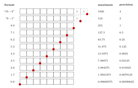
Figure 28: The binary point moving across the same eight bits. The highest bit is worth 2 to the m minus 1 and the lowest is worth 2 to the minus n, so each step of the point to the right doubles both the maximum value and the gap between neighbouring values. At 8.0 the byte is an ordinary unsigned integer. Past that, in the 9.-1 and 10.-2 formats, the point lies beyond the byte, with one or two bits that are always 0 between them (drawn dashed), so only even numbers or multiples of 4 can be held, up to 510 or 1020. At the other end, 0.8 holds only values below 1, in steps of 1/256.
Worked examples
Worked: 4.375 in three formats
Write 4.375 in the 8-bit unsigned formats 4.4, 5.3 and 3.5.
\(4.375 = 100.011_2\) (Method 1 or 2 above). It needs 3 integer bits and 3 fractional bits, so it fits all three formats exactly; only the padding changes.
| Format | Bits | Check |
|---|---|---|
| 4.4 | 0100.0110 |
\(70 / 16 = 4.375\) |
| 5.3 | 00100.011 |
\(35 / 8 = 4.375\) |
| 3.5 | 100.01100 |
\(140 / 32 = 4.375\) |
In 2.6 it would not fit: 4 needs a bit worth 4, and 2.6’s highest bit is worth 2.
Worked: choosing a format
A byte must hold a percentage, 0 to 100, as precisely as possible. Which unsigned format? And for a signed value between \(-3\) and \(+3\)?
Percentage. The maximum must reach 100. Going down the table, 7.1 reaches 127.5 and 6.2 only 63.75, so 7.1, with a precision of 0.5.
\(\pm 3\). In two’s complement, 3.5 runs from \(-4\) to \(3.96875\) and 2.6 from \(-2\) to \(1.984375\). So two’s complement 3.5, with a precision of \(\tfrac1{32}\).
In both cases the rule is: take the smallest \(m\) that still reaches the largest value, because every integer bit not needed is a fractional bit lost.
Worked: 0.1 has no exact form
Store 0.1 in unsigned 4.4.
Method 2: \(0.1 \times 16 = 1.6\), not a whole number, so 0.1 cannot be stored exactly. The nearest step is \(2/16 = 0.125\) (0000.0010); truncating gives \(1/16 = 0.0625\) (0000.0001). Repeated doubling shows why no number of bits is enough: \(0.1 \to 0.2 \to 0.4 \to 0.8 \to 1.6 \to 1.2 \to 0.4 \to \dots\) gives \(0.000110011\ldots_2\), with 0011 repeating for ever. A fraction is finite in binary only when its denominator is a power of 2, so 0.375 (\(\tfrac38\)) is exact and 0.1 (\(\tfrac1{10}\)) is not.
Why use it
Fixed point needs no new hardware. Two values in the same \(m.n\) format add and subtract with the ordinary integer adder, because the points line up; only the reading changes. That makes it the natural choice for fractions on a small processor like the AVR, which has integer instructions only (instruction-set-architecture). The price is the trade-off above: the range and the precision are fixed once the format is chosen, and a value too large or too small for it simply cannot be held. floating-point-numbers stores the position of the point alongside the digits so that it can move.
Common mistakes
- Reading the fraction bits as a whole number.
.011is \(\tfrac14 + \tfrac18 = 0.375\), not “0.3”. - Forgetting that the point is an agreement. A byte has no point in it; the same
10110101is 181, 22.625 or \(-9.375\) depending on the format chosen. - Giving the MSB a positive weight in two’s complement. In two’s complement 5.3, the first bit is worth \(-16\); only that bit is negative, and the fraction bits still add.
- Negating by adding 1 to the integer part. The 1 is added in the last place, \(2^{-n}\).
- Taking the maximum as \(2^m\). It is one step short: \(2^m - 2^{-n}\) (31.875 for 5.3, not 32).
- Reading the doubling remainders in the wrong order. For a fraction the bits come out left to right, the first one just after the point. That is the opposite of repeated division for a whole number.
- Expecting every decimal fraction to be exact. Only fractions with a power-of-2 denominator are.
See also
- floating-point-numbers — letting the point move, IEEE 754
- binary-number-representations — place values, unsigned and two’s complement whole numbers
- instruction-set-architecture — the AVR’s 8-bit integer data type, the only one it has in hardware
- 2026-10-19-floating-point-numbers — Lecture 23
Flip-Flops and Latches
Flip-flops and latches are the storage elements — the circuits that let a design remember a value even after the input that produced it has changed. They’re what turns a combinational circuit into a sequential circuit.
Introduced in Lecture 5, 2026-08-10-introduction-to-sequential-circuits.
The D flip-flop
The D flip-flop is the only flip-flop type covered in this course. Its symbol is a rectangle with:
- D — the data input, on the left.
- Q — the output, on the right.
- CLK — the clock, a control input on the left, drawn with a small triangular wedge where it meets the box.
How it works: Q copies the value of D (and remembers it) whenever CLK goes from 0 to 1 — the rising edge. In between clock edges the flip-flop is not responsive, so it holds the stored value. Q changes only on that 0→1 transition.
Summary: a D flip-flop remembers a single bit — either a “1” or a “0”. It keeps that value until the next clock edge, at which point the D input is transferred to output Q.
- To remember \(n\) bits you need \(n\) D flip-flops.
- An \(n\)-bit register is (by definition) \(n\) D flip-flops. See shift-registers.
- Flip-flops can themselves be made out of logic gates — see the SR latch and A real D flip-flop below.
Characteristic table
A characteristic table defines the operation of a flip-flop in tabular form. The left column is the input; the right column, \(Q(t+1)\), is the next value of Q: what the output will be on the next clock edge (i.e. when CLK goes 0→1).
| D | Q(t+1) | |
|---|---|---|
| 0 | 0 | Reset |
| 1 | 1 | Set |
That is the whole behaviour: the flip-flop is reset (to 0) or set (to 1) according to D, at the clock edge.
A flip-flop’s next-state column is written \(Q(t+1)\) here. The state tables of state-machines and counters call the same thing Next State. The course uses both names (see csse2010-diagram-notation).
Worked waveform
D is 0, 0, then 1, 1 across a clock with two rising edges. CLK starts low, pulses high, goes low, then pulses high again after D has risen.
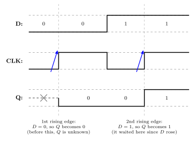
Figure 29: A D flip-flop waveform. The dashed verticals are the two rising clock edges, and the arrows mark them. Q is undefined (drawn dashed, with a cross) until the first edge. The point of the figure is the middle: D rises well before the second edge, and Q does not follow until that edge arrives.
| Clock edge | D at that edge | Q after |
|---|---|---|
| (before the first edge) | — | unknown/undefined |
| 1st rising edge | 0 | 0 |
| 2nd rising edge | 1 | 1 |
Before the first rising edge Q is undefined, because nothing has been clocked in yet; an “X” marks that stretch. Between the two rising edges Q stays 0 even though D has already risen to 1: the flip-flop is only sensitive at the edge. Remember: Q changes only when the clock (CLK) goes from 0 to 1.
A second, harder worked waveform — four clock edges, with D both rising and falling between them — is in 2026-08-10-introduction-to-sequential-circuits.
Other flip-flop types
Other types exist — JK flip-flops and T flip-flops — but they are not covered in this course. Only the D flip-flop is used.
Latches vs flip-flops
- Latches are level triggered devices — they latch the output and respond to changes of logic levels on the inputs.
- A latch circuit can be modified so that it becomes sensitive to an edge (a momentary transition) of a control input, i.e. a clock signal. Such circuits are called flip-flops.
- A flip-flop can store 1 bit of information while being sensitive to a clock edge — it changes its output only at the clock edges, based on the inputs.
- So: latches are level triggered; flip-flops are edge triggered.
A clock signal has two edges:
| Edge | Transition |
|---|---|
| Positive (rising) edge | 0 → 1 |
| Negative (falling) edge | 1 → 0 |
A D flip-flop can therefore be positive edge triggered or negative edge triggered. In a positive edge triggered D flip-flop, D is copied to Q at the positive edge of the clock; in between clock edges the flip-flop is not responsive, thus stores the value.
The state of a flip-flop is the value it is storing. Flip-flops are more useful than latches in practice.
Symbols used
Four related symbols, all drawn as a rectangle with D in at the top left, Q out at the top right, and a clock input CK at the bottom left. What distinguishes them is the marking on that CK input.
Figure 30: The four latch and flip-flop symbols, with the clock pin labelled CK (the course writes this pin CLK elsewhere). The wedge and the bubble read independently: the wedge says edge-triggered, therefore flip-flop; the bubble says inverted, therefore falling edge or low level. The reading under each symbol follows from those two rules.
| Symbol | CK input marking | Device | Triggered on |
|---|---|---|---|
| (a) | plain input | Latch | High level of CK |
| (b) | bubble (inversion circle) | Latch | Low level of CK |
| (c) | triangle/wedge | Flip-flop | Rising (positive) edge of the clock |
| (d) | bubble + triangle | Flip-flop | Falling (negative) edge of the clock |
The two markings read independently and are the whole key to the notation:
- The triangle indicates edge-triggered, and therefore that the device is a flip-flop rather than a latch. No triangle means level-triggered, i.e. a latch.
- The bubble indicates inversion, i.e. the falling edge (or the low level) rather than the rising edge (or the high level).
The SR latch (cross-coupled NOR gates)
Structure: two 2-input NOR gates cross-coupled.
- The top NOR gate takes \(S\) as one input and the bottom gate’s output as its other input; its output is \(\bar Q\).
- The bottom NOR gate takes \(R\) as one input and the top gate’s output (\(\bar Q\)) as its other input; its output is \(Q\).
So each gate’s output feeds back into the other gate’s input — that feedback loop is what stores the bit.
Figure 31: The SR latch: two cross-coupled NOR gates, with the NOR truth table to remember and the two special cases the analysis needs. Between them they are the whole analysis: a NOR with a 0 on one input passes the other input inverted, and a NOR with a 1 on one input is pinned to 0. Where the two feedback wires cross there is no junction dot, so it is two wires passing, not a connection.
The analysis needs both identities in the figure. Together they are what makes each row fall out in a line. Both are just De Morgan applied to a NOR (see boolean-algebra): \(\overline{A+B} = \bar A \cdot \bar B\).
The truth table:
| S | R | Q | \(\bar Q\) | Meaning |
|---|---|---|---|---|
| 0 | 0 | \(Q_{n-1}\) | — | Storage / remember |
| 0 | 1 | 0 | 1 | Reset |
| 1 | 0 | 1 | 0 | Set |
| 1 | 1 | — | — | Invalid \(\times\) |
\(Q_{n-1}\) means “whatever \(Q\) was before” — the hold row’s entry is not a bit but a reference to the previous value. Three cells are left blank: \(\bar Q\) in the hold row, and both outputs in the last row, which is Invalid.
Reasoning for each row, using the two identities above:
- \(S=0, R=0\): each gate has a 0 on its external input, so each is an inverter of the other’s output — \(\bar Q = \overline{Q}\) and \(Q = \overline{\bar Q}\). Both \(Q=1\) and \(Q=0\) satisfy that, so the latch simply holds whatever it already had. This row is the whole point of the circuit: it is the row in which the latch remembers.
- \(S=1, R=0\): the top gate has a 1 on an input, so \(\bar Q = 0\) regardless. The bottom gate then sees \(R=0\) and \(\bar Q=0\), so \(Q=1\). \(S\) sets the latch.
- \(S=0, R=1\): mirror image — the bottom gate has a 1 on an input, so \(Q=0\); the top gate then sees \(S=0\) and \(Q=0\), so \(\bar Q=1\). \(R\) resets the latch.
- \(S=1, R=1\): both gates have a 1 on an input, so both outputs are 0: \(Q = 0\) and \(\bar Q = 0\). That result is what condemns the combination: the two outputs are supposed to be complements and here they are equal, so the labels \(Q\) and \(\bar Q\) stop meaning anything. Worse, what happens after both inputs return to 0 simultaneously is not uniquely determined (the two gates race), so the resulting state is indeterminate. Hence invalid — a combination you must not apply.
This circuit is the active high SR latch: the inputs do their job when driven to 1, and the resting/hold condition is \(S=R=0\). That name is what distinguishes it from the NAND version below.
The SR latch from NAND gates (active low)
Exercise: analyse the SR latch circuit when the NOR gates are replaced with NAND gates, and complete the truth table. The answer circuit is below. The gate symbols are not merely swapped: the inputs are relabelled \(\bar S\) and \(\bar R\), and which gate’s output is called \(Q\) is swapped, so that the set/reset roles survive the change.
Figure 32: The NAND SR latch, the active low SR latch, with the NAND truth table and the two identities that drive the analysis. Compare against the NOR version: the gate outputs have swapped names, so the top gate now produces Q, and the inputs are drawn overlined because they are active low.
Worked through with the two NAND identities in the figure:
| \(\bar S\) | \(\bar R\) | Q | \(\bar Q\) | Meaning |
|---|---|---|---|---|
| 0 | 0 | 1 | 1 | Invalid — outputs not complementary |
| 0 | 1 | 1 | 0 | Set (\(\bar S\) asserted) |
| 1 | 0 | 0 | 1 | Reset (\(\bar R\) asserted) |
| 1 | 1 | \(Q_{n-1}\) | — | Storage / remember |
(Rows in ascending binary order of the inputs, which is what every truth table in the course does — see csse2010-diagram-notation.)
- \(\bar S = \bar R = 1\): each gate has a 1 on its external input, so each inverts the other’s output — the same self-consistent pair as the NOR latch’s \(S=R=0\) row. Hold.
- \(\bar S = 0\): the top gate is pinned to 1, so \(Q = 1\); the bottom gate then sees \(\bar R = 1\) and \(Q = 1\), so \(\bar Q = 0\). Set.
- \(\bar R = 0\): mirror image — \(\bar Q = 1\), and the top gate then gives \(Q = 0\). Reset.
- \(\bar S = \bar R = 0\): both gates pinned to 1, so \(Q = \bar Q = 1\). Same objection as before, so invalid.
The headline result, and the reason the inputs are drawn overlined: with NAND gates the inputs become active low. The latch rests (holds) at \(\bar S = \bar R = 1\) instead of at \(S=R=0\), and the forbidden combination moves from both-high to both-low. Everything else — set, reset, hold, one invalid corner — is the same circuit doing the same job.
This active-low convention is general: it is why the 74HCT74’s asynchronous pins are \(\overline{\text{SET}}\) and \(\overline{\text{CLR}}\) (see device-pinouts). The SET and CLR inputs are typically active low.
A real D flip-flop
A real D flip-flop is built from cross-coupled NAND gates — six NAND gates in three cross-coupled pairs: two input latches driven by D and CLK, and a third pair forming the output latch that carries \(Q\) and \(\bar Q\). That is the same storage idea as the SR latch above, wrapped in enough extra gating to make it respond to an edge rather than a level.
As well as D, CLK and the outputs \(Q\) and \(\bar Q\), it has two extra inputs:
- \(\overline{\text{PRE}}\) (Preset) — forces \(Q\) to 1.
- \(\overline{\text{CLR}}\) (Clear) — forces \(Q\) to 0.
Both are drawn with overbars and with a bubble on the pin, i.e. they are active low, and both are asynchronous: they act on the latch directly, independent of the clock, rather than waiting for a clock edge. They run straight into the NAND gates of the latches, bypassing the D/CLK path entirely — \(\overline{\text{PRE}}\) reaches the gate that produces \(Q\) and \(\overline{\text{CLR}}\) the gate that produces \(\bar Q\), which is exactly how each forces its output.
The two things to remember about these pins: they are active low inputs and asynchronous inputs.
Figure 33: The D flip-flop symbol with its asynchronous pins, CLR on top and PRE underneath. The 74HCT74 in device-pinouts is drawn the other way up (SET on top, CLR below), which is the course’s usual order; the course is also inconsistent about the naming (PRE/CLR against SET/CLR). The three consequences of the pins being asynchronous and active low are on the right.
Both pins being asserted at once (\(\overline{\text{PRE}} = \overline{\text{CLR}} = 0\)) is the same kind of contradiction as \(S=R=1\) on the NOR latch — it demands \(Q=1\) and \(Q=0\) simultaneously — and is likewise a combination to avoid. It follows from the SR-latch analysis above.
When neither is needed they can simply be omitted from a drawing: the course’s Device Pinouts and Symbols sheet says so in words, and its own logic-diagram symbol for a D flip-flop leaves them off. See device-pinouts and circuit-schematics.
D flip-flop chips
- 74HCT74 — dual D flip-flop (two independent D flip-flops in a 14-pin package), each with its own clock, its own CLR and its own PR (preset), and \(Q\)/\(\bar Q\) outputs. Pinout and schematic symbol in device-pinouts.
- 74HCT273 — eight D flip-flops in a 20-pin package, so it can hold one byte (8 bits) of information. It is not in the course’s device-symbols document, so there is no pinout for it here.
The full symbol set is in the device symbols PDF on Blackboard.
See also
- 2026-08-10-introduction-to-sequential-circuits — Lecture 5, where all of this is introduced
- sequential-circuits — what you build once you have a storage element
- shift-registers · counters · state-machines
- memory-technologies — static RAM, a memory that keeps each bit in a latch
- week3-lab-logisim-and-flip-flops — the lab that simulates these circuits
- logic-gates · boolean-algebra — the NOR/NAND behaviour the latch analysis rests on
- timing-diagrams — how to read and draw the waveforms above
- csse2010-diagram-notation — the drawing conventions these figures follow
Floating-Point Numbers
How a computer holds numbers as large as \(6 \times 10^{23}\) and as small as \(3.6 \times 10^{-4}\) in the same few bytes: store the digits and the position of the point separately, as scientific notation in binary. This note covers why a fixed point is not enough, scientific notation and normalisation, where the word “mantissa” comes from, the IEEE 754 single and double precision formats (sign, excess-127 or excess-1023 exponent, mantissa with an implicit leading 1, and why the fields are in that order), converting in both directions, the special values (zero, subnormal numbers, infinity and NaN), what finite precision does to arithmetic, the family of formats from quarter to octuple precision with every quarter-precision value listed, and floating point in C and on the AVR. Fixed point, the alternative this improves on, is in fixed-point-numbers. The excess notation behind the exponent is in binary-number-representations. First met in 2026-10-19-floating-point-numbers.
Why the point has to float
A fixed-point format spends its bits once and for all between range and precision (fixed-point-numbers). Real quantities do not cooperate.
- Avogadro’s number is \(6.02214076 \times 10^{23}\), written out
602214076000000000000000. As a whole number it needs 79 bits (\(\log_2 \approx 78.99\)), and only its first nine digits carry any information. - The volume of a cup is about \(0.00036\ \text{m}^3\). In fixed point its first 1 is in the 12th place after the point (\(2^{-12} \approx 0.000244\)), so it needs at least 12 fractional bits just to be non-zero, and more for any precision.
To hold both in one format, a fixed-point number would need about 79 integer bits and a few dozen fractional bits, nearly all of them zero in any given value. The way out is the one people already use: write the significant digits once and say separately where the point goes.
Scientific notation
Everyday language already lets the point move. SI prefixes do it in words: a kilometre is \(10^3\) m, a milligram \(10^{-3}\) g, and the scale runs out to femto (\(10^{-15}\)), yocto (\(10^{-24}\)) and beyond. The number in front stays a convenient size and the prefix carries the scale.
Scientific notation does it in symbols:
\[\text{value} = \text{significant digits} \times \text{base}^{\text{exponent}}\]
so Avogadro’s number is \(6.02 \times 10^{23}\) and the cup is \(3.6 \times 10^{-4}\ \text{m}^3\). The digits say what the number is and the exponent says how big. Moving the point one place left and adding 1 to the exponent leaves the value unchanged, which is exactly the freedom fixed point lacks.
Normalisation
That freedom means one value has many spellings: \(602 \times 10^{21} = 60.2 \times 10^{22} = 6.02 \times 10^{23} = 0.602 \times 10^{24}\). A normalised number picks one of them: exactly one non-zero digit before the point. In decimal that puts the digits in the range \([1, 10)\), and \(6.02 \times 10^{23}\) is the normalised form.
In binary the same rule gives the range \([1, 2)\). The only non-zero binary digit is 1, so a normalised binary number always looks like \(1.xxxx_2 \times 2^e\). Something like \(3.985 \times 2^{77}\) is not normalised in binary, even though 3.985 would be fine in front of a power of 10: it should be \(1.993 \times 2^{78}\). Halving the digits and adding one to the exponent, or doubling and subtracting one, moves between the spellings.
Normalising gives every value a single representation, so no bit patterns are wasted on duplicates, and it guarantees no precision is spent on leading zeros. In binary it does one more thing, used below: the first digit is always 1, so it need not be stored.
Why “mantissa”
The digits part of a floating-point number is called the mantissa (the IEEE standard’s own term is significand). The word comes from logarithm tables.
Before calculators, multiplication was done with \(\log(a \times b) = \log a + \log b\): look up two logarithms, add them, and look up the antilog. A printed table only needs the logarithms of 1.00 to 9.99, because scaling by 10 only adds 1 to the logarithm:
| \(x\) | \(\log_{10} x\) | Integer part | Fractional part |
|---|---|---|---|
| 0.123 | \(-0.9101\) | \(-1\) | \(0.0899\) |
| 1.23 | \(0.0899\) | 0 | \(0.0899\) |
| 12.3 | \(1.0899\) | 1 | \(0.0899\) |
| 123 | \(2.0899\) | 2 | \(0.0899\) |
The fractional part, the same 0.0899 for all four, depends only on the significant digits 1, 2, 3, and it was called the mantissa. The integer part, which only says where the point goes, was the characteristic. A four-figure table lists the mantissas: the row for 12 and the column for 3 give 0899, meaning \(\log_{10} 1.23 = 0.0899\). (For 0.123 the log is \(0.0899 - 1 = -0.9101\); tables wrote it \(\bar{1}.0899\) to keep the mantissa visible.)
A floating-point number splits the same way: digits that say what, an exponent that says where the point goes. The digits inherited the name, although strictly the old mantissa was a logarithm and the new one is the digits themselves.
IEEE 754
Almost every computer stores floating point in the formats of the IEEE 754 standard. A number is stored as three fields, sign, exponent and mantissa, and stands for
\[(-1)^S \times 1.M_2 \times 2^{E - \text{bias}}\]
| Format | Bits | Sign | Exponent | Mantissa | Bias |
|---|---|---|---|---|---|
| Single precision | 32 | 1 | 8 | 23 | 127 |
| Double precision | 64 | 1 | 11 | 52 | 1023 |
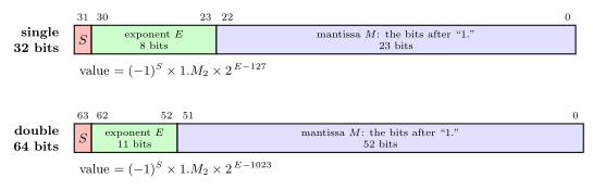
Figure 34: The IEEE 754 single and double precision layouts, MSB on the left, with the bit number at each field boundary. The sign bit is 0 for plus and 1 for minus. The exponent field E holds the true exponent plus the bias, 127 or 1023. The mantissa field M holds only the bits after the point, because a normalised binary mantissa always starts with a 1 that does not need storing. Reading a pattern means putting those three back together as (-1) to the S, times 1.M, times 2 to the E minus the bias. The exponent and mantissa are drawn to scale within each row, double precision at half the scale of single; the sign bit is drawn wider than one bit so it can be labelled.
The biased exponent
The exponent can be negative, so it needs a signed format. IEEE uses excess (biased) notation: the field holds the true exponent plus a fixed bias,
\[E = e + \text{bias}, \qquad \text{bias} = 2^{k-1} - 1 \text{ for a } k\text{-bit exponent}.\]
So single precision is excess-127 and double precision excess-1023. A true exponent of 4 is stored as \(4 + 127 = 131 = 10000011_2\); a true exponent of \(-2\) as \(125 = 01111101_2\).
This is the excess notation of binary-number-representations, with one difference to watch: the bias there is \(2^{k-1}\) (excess-128 for 8 bits), while IEEE uses one less, 127. The stored values 0 and 255 are kept for the special values, so the normal true exponents run from \(1 - 127 = -126\) to \(254 - 127 = +127\).
The implicit leading 1
A normalised binary mantissa is always \(1.xxxx_2\) (normalisation). A bit that is always 1 carries no information, so IEEE does not store it. The mantissa field holds only the bits after the point, and the 1 is put back when the number is read. Single precision therefore has 24 significant bits for the price of 23. The one exception is the subnormal numbers, where the hidden bit is 0.
Why sign, exponent, mantissa
The order is chosen so that floating-point numbers sort like integers. Compare \(1 \times 2^{100}\) with \(3 \times 2^{20}\): the first is far larger, even though its mantissa is smaller, because the exponent decides the scale and the mantissa only refines it. Putting the exponent in the high bits, above the mantissa, means that comparing two patterns as plain integers compares exponents first and mantissas only when the exponents are equal, which is exactly numeric order.
The biased exponent is what makes this work. In excess form a larger exponent is always a larger unsigned field, negative exponents included, so no two’s complement sign gets in the way. The result: for two non-negative floats, the one whose bit pattern is the larger unsigned integer is the larger number, and the integer comparison hardware can sort floats. The quarter-precision table shows it: reading the patterns in counting order reads the values in increasing order. The sign bit comes first so that sign alone splits positive from negative; negative numbers are sign and magnitude, so among them the order reverses.
Encoding: decimal to IEEE
- Convert to binary scientific notation, normalised: \(\pm 1.xxxx_2 \times 2^e\) (fixed-point-numbers for the fraction bits).
- Store the sign: \(+\) gives 0, \(-\) gives 1.
- Store the biased exponent: \(e + 127\) in 8 bits (single) or \(e + 1023\) in 11 bits (double).
- Store the mantissa: drop the leading 1 and pad with zeros on the right to 23 (or 52) bits. Right, because these are fraction bits: zeros after the last 1 do not change the value.
- Group into nibbles and write the 32 bits as 8 hex digits.
And beware of special values: zero, infinity and NaN do not follow these steps (below).
\(-23.25\) worked through these steps to 0xC1BA0000 is in 2026-10-19-floating-point-numbers.
Worked: 5.75 to single precision
Write 5.75 as an IEEE single-precision number in hexadecimal.
- \(5.75 = 101.11_2 = 1.0111_2 \times 2^2\).
- Positive: \(S = 0\).
- \(E = 2 + 127 = 129 = 10000001_2\).
- \(M\) =
0111followed by 19 zeros. 0 10000001 01110000000000000000000=0100 0000 1011 1000 0000 0000 0000 0000=0x40B80000.
Worked: \(-0.375\) to single precision
Write \(-0.375\) as an IEEE single-precision number in hexadecimal.
- \(0.375 = 0.011_2 = 1.1_2 \times 2^{-2}\). The point moves right, so the exponent is negative.
- Negative: \(S = 1\).
- \(E = -2 + 127 = 125 = 01111101_2\).
- \(M\) =
1followed by 22 zeros. 1 01111101 10000000000000000000000=1011 1110 1100 0000 0000 …=0xBEC00000.
Worked: 0.1 to single precision
Write 0.1 as an IEEE single-precision number. Is it exact?
\(0.1 = 0.0\,0011\,0011\,0011\ldots_2\) repeating (fixed-point-numbers), which normalises to \(1.1001\,1001\,1001\ldots_2 \times 2^{-4}\). So \(S = 0\) and \(E = -4 + 127 = 123 = 01111011_2\). The mantissa should be 1001 repeated for ever. Only 23 bits fit:
10011001100110011001100 | 1100… (the bits that do not fit)
What is cut off starts with a 1 followed by more 1s, so it is more than half a unit in the last place, and the stored mantissa rounds up to 10011001100110011001101. The pattern is 0 01111011 10011001100110011001101 = 0x3DCCCCCD, and it stands for \(0.100000001490116\ldots\), not 0.1. 0.1 has no exact binary floating-point form, for the same reason \(\tfrac13\) has no exact decimal one.
Decoding: IEEE to decimal
- Write the hex as 32 bits and split 1 / 8 / 23.
- Sign: 0 is \(+\), 1 is \(-\).
- Exponent: check for all 0s or all 1s (special values); otherwise \(e = E - 127\).
- Mantissa: put back the hidden 1, giving \(1.M_2\).
- Shift the point \(e\) places (right if \(e > 0\)) and convert.
0x422F0000 decoded this way to 43.75 is in 2026-10-19-floating-point-numbers.
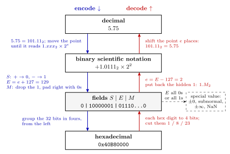
Figure 35: Encoding and decoding are the same four stages walked in opposite directions, shown with 5.75. Encoding (down the left) writes the value in binary and moves the point until one 1 is left in front of it; the sign becomes S, the power of 2 plus 127 becomes E, and the bits after the leading 1 become M, padded with zeros on the right; the 32 bits are then grouped in fours for hex. Decoding (up the right) undoes each step: expand every hex digit to four bits, cut the bits 1 / 8 / 23, take 127 off E and put the hidden 1 back, and shift the point. The one extra step is on the way up: an exponent field of all 0s or all 1s is not a normal number and has to be read as a special value instead.
Worked: 0x41200000
What decimal value does the single-precision pattern
0x41200000hold?
0100 0001 0010 0000 … splits as \(S = 0\), \(E = 10000010_2 = 130\), \(M = 0100\ldots\). So the value is \(+1.01_2 \times 2^{130-127} = 1.01_2 \times 2^3 = 1010_2 = \mathbf{10}\).
Worked: two special patterns
What do
0x80000000and0x7F800000hold?
0x80000000is1 00000000 000…0: exponent all 0s and mantissa 0, with the sign set. It is \(-0\), which compares equal to \(+0\).0x7F800000is0 11111111 000…0: exponent all 1s and mantissa 0, sign clear. It is \(+\infty\). Following steps 4 and 5 blindly would give \(1.0 \times 2^{128}\), which is the mistake the special-value check is there to catch.
Special values
The smallest and largest exponent fields are reserved. What a pattern means then depends on whether the mantissa field is zero. The exponent here is the raw field as stored, with no bias taken off, so the reserved values are 0 (all 0s) and the maximum (all 1s, 255 in single precision):
| Exponent field (as stored) | Mantissa \(= 0\) | Mantissa \(\neq 0\) |
|---|---|---|
| 0 \(\to\) all 0s | \(\pm 0\) | subnormal numbers |
| anything else | normal numbers | normal numbers |
| maximum \(\to\) all 1s (255 for single, 2047 for double) | \(\pm\) infinity | \(\pm\) NaN (not a number) |
This raw field is often called the unbiased exponent, in the sense that the bias has not yet been subtracted; the true exponent of a normal number is the field minus 127 (or 1023).
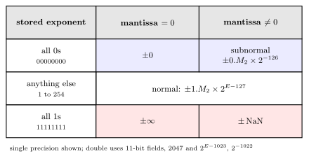
Figure 36: What a floating-point pattern means, decided by the stored exponent field (rows) and whether the mantissa field is zero (columns). Every exponent except all 0s and all 1s gives an ordinary normalised number, with the hidden 1 in front of the mantissa. All 0s gives zero, or a subnormal number with a hidden 0 instead of a 1 and the smallest normal exponent, which is 2 to the minus 126 in single precision. All 1s gives infinity, or NaN when any mantissa bit is set. The sign bit applies in every cell, so there are two zeros, two infinities, and NaNs of either sign.
Zero
Zero cannot be normalised (it has no leading 1), so it gets its own pattern: every exponent and mantissa bit 0. Because the sign bit is separate there are two of them, \(+0\) (0x00000000) and \(-0\) (0x80000000). They compare equal; the sign survives only in things like \(1 / -0 = -\infty\).
Subnormal numbers
With an all-0s exponent and a non-zero mantissa, the number is subnormal (also called denormal):
\[(-1)^S \times 0.M_2 \times 2^{-126} \quad \text{(single precision)}\]
Two rules differ from normal numbers.
- The hidden bit is 0, not 1. This breaks the scientific-notation rule of one non-zero digit before the point, on purpose: it lets values smaller than the smallest normal number be held, with fewer significant bits as they shrink.
- The exponent is \(2^{-126}\), the same as the smallest normal numbers, not \(2^{0-127} = 2^{-127}\) as the excess rule would give. With \(2^{-126}\) the subnormals continue the smallest normal binade at exactly the same spacing, \(2^{-149}\), all the way down to 0, with no gap and no overlap. With \(2^{-127}\) they would be spaced twice as finely and leave a gap below \(2^{-126}\).
The smallest normal single is \(2^{-126} \approx 1.18 \times 10^{-38}\), and the smallest subnormal is \(2^{-23} \times 2^{-126} = 2^{-149} \approx 1.4 \times 10^{-45}\). The effect is easiest to see in quarter precision (figure below).
Infinity
All-1s exponent, zero mantissa: \(\pm\infty\). It is the result when
- a number is too big to store: anything past the largest finite value (about \(3.4 \times 10^{38}\) for single) overflows to \(\infty\);
- a calculation is mathematically infinite: \(1 \div 0 = +\infty\), \(-\log 0 = +\infty\) (\(\log 0 = -\infty\)), \(\tan(\pi/2)\).
On the last: in practice tan(M_PI/2) returns a large finite number, about \(1.6 \times 10^{16}\) in double, because \(\pi/2\) itself cannot be stored exactly and the tangent of the stored value is merely huge.
Infinity behaves sensibly in further arithmetic: \(\infty + 1 = \infty\), \(1 / \infty = 0\), $-< $ every finite number.
NaN
All-1s exponent, non-zero mantissa: NaN, not a number. It is the result of an operation with no meaningful answer:
- \(0 \div 0\), \(0 \times \infty\), \(\infty - \infty\);
- \(\sqrt{-1}\), \(\log(-1)\), \(\sin^{-1} 20\) (no real angle has a sine of 20);
- \(0^0\), as an indeterminate form. IEEE 754’s
powr(0, 0)gives NaN; C’spow(0, 0)returns 1 by convention.
A NaN propagates: any arithmetic with a NaN operand gives NaN, so one bad step poisons everything computed from it, and the NaN at the end shows something went wrong. There are a few exceptions, functions whose answer does not depend on the missing value: pow(NaN, 0) is 1, and fmax(NaN, 3) is 3. Comparisons do not produce NaN at all; they return false. In particular x == x is false when x is NaN, which is the standard test for one (or isnan(x) in C). With 23 mantissa bits there are \(2^{23} - 1\) different NaN patterns per sign, all meaning NaN.
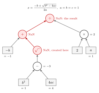
Figure 37: How one NaN poisons a calculation, in the quadratic formula with a = b = c = 1, which has no real root. Arrows show which results feed which operation. The discriminant b squared minus 4ac is -3, an ordinary number. Its square root has no real answer, so that operation creates a NaN. Every operation that then takes the NaN as an operand gives NaN too, so the sum and the final division are NaN. The branch that never touches it, 2a, is still 2. The NaN that comes out at the top is the signal that something went wrong further down. Comparisons are the exception: they do not give NaN but false, so result == result is false for a NaN.
Finite precision
A float has a fixed number of mantissa bits, so most real numbers cannot be represented exactly and are rounded to the nearest value that can (ties go to the neighbour whose last mantissa bit is 0, “round half to even”). The error is relative: single precision keeps 24 significant bits, about 7 decimal digits, wherever the point is; double keeps 53, about 16.
Rounding happens after every operation, and that changes the arithmetic rules.
Division and multiplication need not undo each other. \(10 \div 3 = 3.333\ldots = 11.010101\ldots_2\), which repeats for ever and has to be cut short. In 3-digit decimal the same thing gives \(10 \div 3 = 3.33\) and \(3.33 \times 3 = 9.99 \neq 10\). Whether the binary version lands back on 10 depends on how the roundings fall: for \(10 \div 3 \times 3\) they happen to cancel in single and double, but \((1 \div 41) \times 41 = 0.99999994\) in single, and \((1 \div 49) \times 49 = 0.9999999999999999\) in double. So \((x \div y) \times y\) may not equal \(x\), and code should never test floats for exact equality after arithmetic; it should test whether they are within a tolerance.
The order of operations matters. This is often put loosely as floating point being occasionally non-commutative. Strictly, addition is still commutative (\(a + b = b + a\) always); what fails is associativity: \((A + B) + C\) need not equal \(A + (B + C)\), because the two orders round different intermediate results. In double, \((0.1 + 0.2) + 0.3 = 0.6000000000000001\) while \(0.1 + (0.2 + 0.3) = 0.6\). The order of a long sum changes its answer.
Absorption
If \(X \gg \delta\), then \((X + \delta) - X\) can be 0. Near \(X\) the representable values are spaced by about \(X \times 2^{-23}\) (single). If \(\delta\) is less than half that gap (or exactly half, when the tie goes to \(X\)), \(X + \delta\) rounds straight back to \(X\), and subtracting \(X\) leaves nothing: \(\delta\) has been absorbed.
- Single precision: \(2^{24} = 16\,777\,216\), and the gap there is 2. So \(2^{24} + 1\) is a tie between \(16\,777\,216\) and \(16\,777\,218\), rounds to the even one, and \((2^{24} + 1) - 2^{24} = 0\). The same happens with \(10^8 + 1 - 10^8\).
- It also breaks associativity: \((2^{24} + 1) + 1 = 2^{24}\), since each 1 is absorbed in turn, but \(2^{24} + (1 + 1) = 2^{24} + 2\).
So adding many small numbers to a large total can lose them all; adding the small ones together first keeps them.
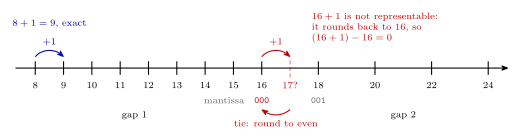
Figure 38: Absorption, shown on the quarter-precision values between 8 and 24. Between 8 and 16 neighbouring values are 1 apart, so 8 + 1 = 9 is exact. Between 16 and 32 they are 2 apart, and 16 + 1 = 17 falls exactly halfway between 16 and 18. The tie goes to the neighbour whose last mantissa bit is 0: 16 has mantissa field 000 and 18 has 001, so 16 + 1 rounds back to 16 and (16 + 1) - 16 = 0. The same thing happens in any format whenever the number added is less than half the gap at the size of the larger number, or exactly half with the tie going back down.
The formats compared
IEEE 754 defines a family of binary formats that differ only in field widths. Each follows the same rules: bias \(2^{k-1} - 1\) for a \(k\)-bit exponent, hidden 1, the same special values. With \(k\) exponent bits and \(m\) mantissa bits:
- the next value after 1 is \(1 + 2^{-m}\), the precision near 1;
- the largest finite value is \((2 - 2^{-m}) \times 2^{\text{bias}}\): all-1s mantissa, the exponent field one below all 1s.
| Quarter | Half | Single | Double | Quadruple | Octuple | |
|---|---|---|---|---|---|---|
| Total bits | 8 | 16 | 32 | 64 | 128 | 256 |
| Sign bits | 1 | 1 | 1 | 1 | 1 | 1 |
| Exponent bits | 4 | 5 | 8 | 11 | 15 | 19 |
| Mantissa bits | 3 | 10 | 23 | 52 | 112 | 236 |
| Bias | 7 | 15 | 127 | 1023 | 16383 | 262143 |
| Next after 1 | \(1 + \tfrac18 = 1.125\) | \(1 + \tfrac1{1024} \approx 1.001\) | \(1 + 2^{-23}\) \(\approx 1 + 1.2 \times 10^{-7}\) | \(1 + 2^{-52}\) \(\approx 1 + 2.2 \times 10^{-16}\) | \(1 + 2^{-112}\) \(\approx 1 + 1.9 \times 10^{-34}\) | \(1 + 2^{-236}\) \(\approx 1 + 9.1 \times 10^{-72}\) |
| Maximum | 240 | 65504 | \(\approx 3.4 \times 10^{38}\) | \(\approx 1.8 \times 10^{308}\) | \(\approx 1.2 \times 10^{4932}\) | \(\approx 1.6 \times 10^{78913}\) |
| Use | ultra rare | rare | common | common | rare | ultra rare |
Quarter precision is not one of the standard’s formats. It is an 8-bit format built by the same rules (1 sign, 4 exponent, 3 mantissa bits, bias 7), small enough to list every value (below). Half precision appears in graphics and machine learning, where memory matters more than digits; single and double are what ordinary code uses.
The maximum grows with the exponent width and the precision with the mantissa width. Each extra exponent bit doubles the bias and so roughly squares the maximum: \(2^{8} \to 2^{16} \to 2^{128} \to 2^{1024}\) as the exponent goes 4, 5, 8, 11 bits. The quarter maximum is \(1.875 \times 2^7 = 240\) and the half maximum \((2 - 2^{-10}) \times 2^{15} = 65504\).
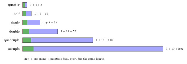
Figure 39: The six formats drawn to one scale, one bit per unit of length, with the sign in red, the exponent in green and the mantissa in blue. As the formats double in size, nearly all of the new bits go to the mantissa: the exponent only grows from 4 to 19 bits while the mantissa grows from 3 to 236. A few exponent bits already give an enormous range, because each one doubles the largest power of 2; the precision needs many more bits, because each mantissa bit only halves the gap between neighbouring values.
Every quarter-precision value
Quarter precision has only 256 patterns, so every value can be listed. Each row is a sign bit (0 here) and a 4-bit exponent field; each column is the 3-bit mantissa field. A normal row with stored exponent \(E\) holds \(1.M_2 \times 2^{E-7}\). The first row (in italics) is the subnormals, \(0.M_2 \times 2^{-6}\), and the last row is infinity and NaN. The negative values are the same table with the sign bit set.
| Sign, exponent | …000 |
…001 |
…010 |
…011 |
…100 |
…101 |
…110 |
…111 |
|---|---|---|---|---|---|---|---|---|
0 0000 |
0 | 0.001953125 | 0.00390625 | 0.005859375 | 0.0078125 | 0.009765625 | 0.01171875 | 0.013671875 |
0 0001 |
0.015625 | 0.017578125 | 0.01953125 | 0.021484375 | 0.0234375 | 0.025390625 | 0.02734375 | 0.029296875 |
0 0010 |
0.03125 | 0.03515625 | 0.0390625 | 0.04296875 | 0.046875 | 0.05078125 | 0.0546875 | 0.05859375 |
0 0011 |
0.0625 | 0.0703125 | 0.078125 | 0.0859375 | 0.09375 | 0.1015625 | 0.109375 | 0.1171875 |
0 0100 |
0.125 | 0.140625 | 0.15625 | 0.171875 | 0.1875 | 0.203125 | 0.21875 | 0.234375 |
0 0101 |
0.25 | 0.28125 | 0.3125 | 0.34375 | 0.375 | 0.40625 | 0.4375 | 0.46875 |
0 0110 |
0.5 | 0.5625 | 0.625 | 0.6875 | 0.75 | 0.8125 | 0.875 | 0.9375 |
0 0111 |
1 | 1.125 | 1.25 | 1.375 | 1.5 | 1.625 | 1.75 | 1.875 |
0 1000 |
2 | 2.25 | 2.5 | 2.75 | 3 | 3.25 | 3.5 | 3.75 |
0 1001 |
4 | 4.5 | 5 | 5.5 | 6 | 6.5 | 7 | 7.5 |
0 1010 |
8 | 9 | 10 | 11 | 12 | 13 | 14 | 15 |
0 1011 |
16 | 18 | 20 | 22 | 24 | 26 | 28 | 30 |
0 1100 |
32 | 36 | 40 | 44 | 48 | 52 | 56 | 60 |
0 1101 |
64 | 72 | 80 | 88 | 96 | 104 | 112 | 120 |
0 1110 |
128 | 144 | 160 | 176 | 192 | 208 | 224 | 240 |
0 1111 |
Inf | NaN | NaN | NaN | NaN | NaN | NaN | NaN |
What the table shows:
- Each row is a binade, the values from one power of 2 up to the next, and it holds eight equally spaced values. The spacing doubles from each row to the next: \(\tfrac18\) between 1 and 2, \(\tfrac14\) between 2 and 4, and 16 between 128 and 240. The relative precision is the same in every row, which is the whole point of floating point.
- Exponent field 0111 is the row of 1, because \(7\) is the bias: \(2^{7-7} = 1\).
- Counting up through the patterns counts up through the values, row by row (why this order).
- The subnormal row has the same spacing as the row after it, \(\tfrac1{512}\), and reaches down to 0. That is the effect of giving subnormals the exponent \(2^{-6}\) rather than \(2^{-7}\).
- The largest finite value is 240, and the next pattern up is infinity. Anything at or above 248, halfway from 240 to the next step, overflows.
- Not every whole number is here. 17, 19 and 33 are missing; between 16 and 32 only the even numbers can be held.
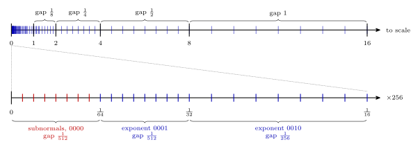
Figure 40: The positive quarter-precision values on a number line. Top: 0 to 16 to scale. Every binade from one power of 2 to the next holds eight evenly spaced values, so the gap doubles at each power of 2, from 1/8 between 1 and 2 to 1 between 8 and 16, and the values crowd together towards 0. Bottom: the stretch from 0 to 1/16 magnified 256 times, so that 1/16 lands directly under 16. The subnormals (exponent field 0000) fill the space below the smallest normal value, 1/64, with the same gap of 1/512 as the first normal binade, so the spacing carries on evenly down to 0 instead of leaving a hole.
Worked: rounding in quarter precision
In quarter precision, what are \(16 + 1\), \(13 \div 3\), and then that quotient times 3?
- \(16 + 1\). Between 16 and 32 the values are 2 apart. 17 is exactly halfway between 16 (mantissa
000) and 18 (mantissa001); the tie goes to the even mantissa, 16. The 1 has been absorbed. - \(13 \div 3 = 4.333\ldots\) Between 4 and 8 the values are 0.5 apart, and 4.333 is nearer 4.5 than 4. So the quotient is 4.5.
- \(4.5 \times 3 = 13.5\). Between 8 and 16 the values are 1 apart, and 13.5 is a tie between 13 (
101) and 14 (110); it goes to the even mantissa, 14. So \((13 \div 3) \times 3 = 14\), not 13.
Floating point in C and on the AVR
C has two floating-point types, float and double. They are usually IEEE single and double precision, but the C standard only sets minimums. Simplified:
floatmust represent numbers up to \(10^{37}\) while keeping 6 decimal digits of accuracy;doublemust represent numbers up to \(10^{37}\) while keeping 10 decimal digits, and must not be less accurate thanfloat.
Single precision meets the first easily (about 7 digits, up to \(3.4 \times 10^{38}\)), and double the second (about 16 digits).
On the AVR, avr-gcc makes double the same as float: 32-bit single precision. That is strictly against the standard, since single precision has about 7 digits, not 10. A program that moves to the AVR from a desktop and relies on double silently loses half its digits (c-language-basics).
GCC also offers _Float16 and __float128, for half and quadruple precision, on targets that support them. There is no C type for quarter or octuple precision.
Prefer integer arithmetic
The AVR has no floating-point hardware. Its only data type in hardware is the 8-bit integer (instruction-set-architecture), so every float operation is a call to a library routine that unpacks the fields, aligns, adds or multiplies the mantissas with integer instructions, renormalises, rounds and checks for special values. Compare two lines that give the same result for every input:
PORTB = PINA / 3;        /* integer division:  about 8 instructions, no branches */
PORTB = PINA * 0.334f;   /* floating point:    300+ instructions, with branches   */
The second converts the byte to a float, calls the software multiply, and converts the result back, and each of those steps is a routine full of tests and loops. Its running time also varies with the input, which matters in an interrupt handler or a timing loop. The first needs no library at all: a compiler turns division by a constant into a multiplication by a fixed-point reciprocal and a shift. One way for a byte: \(x \div 3 = (x \times 171) \gg 9\), since \(171/512 = 0.33398\ldots\) is just above \(\tfrac13\), and this gives exactly \(\lfloor x/3 \rfloor\) for every \(x\) from 0 to 255. (Checking all 256 inputs also confirms that truncating PINA * 0.334f gives the same answers.)
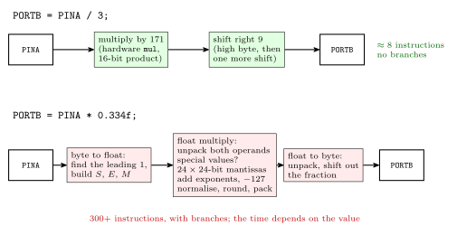
Figure 41: Why the two lines differ so much in cost on the AVR. Dividing a byte by 3 can be done with the hardware 8-by-8 multiply and a shift: multiply by 171 and shift right 9 places, which is the same as taking the high byte of the product and shifting it once more. That is a few instructions with no branches, taking the same time for every input. The float version has no hardware to use. The byte is first converted to a float, which means finding its leading 1 and building the sign, exponent and mantissa fields. The multiply is a library routine that unpacks both operands, tests for special values, multiplies the 24-bit mantissas with 8-bit multiplies, adds the exponents and takes off one bias, then normalises, rounds and packs the result. A third routine converts back to an integer. Each step is a loop or a chain of tests, so the time also depends on the value.
So on a small microcontroller, work in integers or fixed-point-numbers wherever the result can be the same: scale a value so that the fraction becomes whole numbers (millivolts instead of volts, tenths of a degree), and divide or shift at the end.
Common mistakes
- Normalising binary to \([1, 10)\). In binary the mantissa must be in \([1, 2)\): \(3.985 \times 2^{77}\) is not normalised; \(1.993 \times 2^{78}\) is.
- Storing the hidden 1. The mantissa field holds only the bits after the point.
- Using a bias of 128. IEEE single is excess-127 and double excess-1023, one less than the \(2^{k-1}\) of plain excess notation.
- Forgetting the bias when decoding. An exponent field of 132 means \(2^5\), not \(2^{132}\).
- Padding the mantissa on the left. The zeros go on the right; they are fraction bits.
- Decoding special patterns as normal numbers. Check the exponent for all 0s or all 1s first:
0x7F800000is infinity, not \(2^{128}\). - Treating a subnormal’s exponent as \(2^{-127}\). It is \(2^{-126}\), with a hidden 0.
- Testing floats for equality. After any arithmetic, compare with a tolerance;
0.1is not exactly 0.1 to begin with. - Assuming addition is associative. The order of a sum can change its result, and a small term can vanish into a large one.
- Expecting 64 bits from
doubleon the AVR. It is 32. - Using floats on the AVR where integers would do. It costs hundreds of instructions per operation.
See also
- fixed-point-numbers — the fixed binary point, \(m.n\) formats, and the range/precision trade-off this escapes
- binary-number-representations — excess notation, sign and magnitude, hex grouping
- c-language-basics —
floatanddoubleamong C’s types, and floating-point constants - instruction-set-architecture — the AVR’s hardware data types, which do not include floating point
- 2026-10-19-floating-point-numbers — Lecture 23
Instruction Set Architecture
The layer where software meets hardware: what a machine instruction is, what an ISA specifies, and why assembly language exists. See cpu-organisation for the hardware below this line and avr-instructions for a real instruction set.
Machine instructions
A machine instruction is a pattern of bits. 0000 1101 0111 0111 is a valid Atmel AVR instruction. Instructions typically consist of two things:
- Opcode (operation code) — defines the operation, e.g. addition.
- Operands — what is being operated on, e.g. particular registers or a memory address.
So one word of machine code says what to do and what to do it to, packed into fixed bit fields. Which bits mean which is entirely a matter of convention — and that convention is the ISA.
The ISA
An Instruction Set Architecture is a specification — i.e. a document. It specifies the interface between hardware and software.
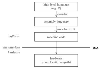
Figure 42: The ISA as an interface. Software above the line is written and compiled without knowing how the hardware works; hardware below the line is designed without knowing what program will run. The only thing both sides must agree on is which bit patterns mean what — and that agreement is a document, not a circuit.
The point of drawing it as a line is that the ISA is the only thing the two sides have to agree on. A compiler writer needs the ISA and nothing else about the chip; a chip designer needs the ISA and nothing else about the programs that will run.
Microarchitecture
Microarchitecture = the architecture of the control unit — i.e. the state machine (gates and flip-flops etc.) that implements the control unit.
This is the same state-machines material from earlier in the course, applied at the scale of a whole processor: the control unit is a state machine whose job is to emit the right control signals, in the right order, for whatever the instruction register holds.
ISA vs microarchitecture
One ISA can be implemented by many different microarchitectures. The specification says what the bit patterns mean; it does not say how a chip must go about honouring them.
| ISA | Implemented by |
|---|---|
| 8086 | many processors, in different ways |
| Pentium | Pentium … Pentium IV … Core2Duo … i7 (each in different ways), various AMD devices, and other manufacturers |
This is why a program compiled decades ago still runs: the ISA held still while the microarchitecture beneath it was rebuilt many times over.
What makes an ISA?
Four things:
- Memory models
- Registers
- Instructions
- Data types
If you know all these details, you can write machine code that runs on the CPU and build the CPU.
This is the completeness test for a specification: both sides of the line in Figure 42 have to be constructible from the document alone, and nothing else about the chip may be needed by either.
1. Memory models
How does memory look to the CPU? Four issues decide it — addressable cell size, alignment, address spaces and endianness — treated in full in memory-models.
2. Registers
Two types of register:
- General purpose — used for temporary results etc. On AVR, r0–r31.
- Special purpose, e.g.
- Program Counter (PC)
- Stack pointer (SP)
- Input/Output registers — 224 of them on the ATmega324A, see avr-io-ports
- Status register — N, Z, C, V among others. Tanenbaum calls this the Program Status Word.
Some other registers are part of the microarchitecture, NOT the ISA — e.g. the Instruction Register (IR). The programmer doesn’t need to know about these, and can’t directly change or use them.
That distinction is the cleanest illustration of what an ISA actually is. The IR unquestionably exists and holds the instruction being executed (fetch-decode-execute-cycle) — but no instruction names it, so it is invisible to software and a chip designer is free to change or remove it. The PC is the opposite case: jmp writes it, so it has to be in the specification. Existing in the hardware is not the criterion; being reachable from an instruction is.
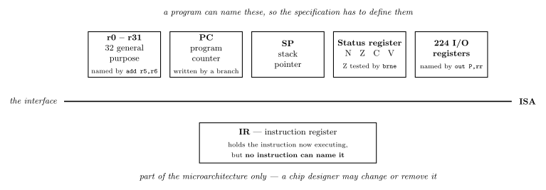
Figure 43: The same interface line as in the previous figure, with the machine’s registers sorted across it. The five above the line are part of the ISA; four of them carry an example of an instruction that names the register, and the SP box carries none. The single box below, the IR, is part of the microarchitecture only. Nothing about a register’s size or importance decides which side it lands on — only whether some instruction can refer to it.
The AVR’s own answer to this pillar — the regularity of r0–r31, the r16–r31 exception, and the X/Y/Z pointer pairs — is in avr-architecture.
3. Instructions
This is the main feature of an ISA. Instruction types include:
| Type | Does |
|---|---|
| Input/Output | communicate with I/O devices/ports |
| Load/Store | move data from/to memory |
| Move | copy data between registers |
| Arithmetic | addition, subtraction, … |
| Logical | Boolean operations |
| Branching | for deciding which instruction to perform next |
The Input/Output row is the one where the AVR’s answer is least obvious. The ATmega324A’s 224 I/O registers are all reachable by ld/st at their data-memory addresses 32 to 255 ($20 to $FF), but only the first 64 also get the short in rd, P / out P, rr form that names an I/O register by its own number P — because P is a six-bit field and \(2^6 = 64\). The other 160, the “extended” I/O registers, can only be reached the long way. The mechanics, the numbering offset and the register list are in avr-io-ports.
With arithmetic and logical merged, the same set can be cut the other way instead — by how many operands an instruction takes:
- Dyadic — two operands, one result
- Monadic — one operand, one result
And instructions use various addressing modes: how an operand says where its value is, covered in addressing-modes.
The AVR instructions met so far, sorted into these boxes, are in avr-instructions.
4. Data types
Numeric
- Integers of different lengths (8, 16, 32, 64 bits), possibly signed or unsigned
- Floating point numbers, e.g. 32 bits (single precision) or 64 bits (double precision)
- Many others not listed
Non-numeric
- Boolean (0 means false, 1 means true) — stored in a whole byte or word
- Bit-map (collection of Booleans, e.g. 8 in a byte)
- Characters
- Pointers (memory addresses)
Different machines provide hardware support for different data types. Two ends of the range:
Intel-64 Architecture
| Data type | 8 bits | 16 bits | 32 bits | 64 bits | 128 bits |
|---|---|---|---|---|---|
| Signed integer | \(\checkmark\) | \(\checkmark\) | \(\checkmark\) | \(\checkmark\) | |
| Unsigned integer | \(\checkmark\) | \(\checkmark\) | \(\checkmark\) | \(\checkmark\) | |
| BCD integer | \(\checkmark\) | ||||
| Floating point | \(\checkmark\) | \(\checkmark\) |
Atmel AVR
| Data type | 8 bits | 16 bits | 32 bits | 64 bits | 128 bits |
|---|---|---|---|---|---|
| Signed integer | \(\checkmark\) | ||||
| Unsigned integer | \(\checkmark\) | ||||
| BCD integer | |||||
| Floating point |
The only data type an AVR supports in hardware is an 8-bit integer, signed or unsigned. There is no 16-bit integer type, no floating point, no BCD.
Other data types can be supported through software! e.g. 16-bit integer operations can be built out of 8-bit operations, using a sequence of instructions — which is exactly what the two-instruction 16-bit addition in avr-instructions does. So the hardware/software line here is about cost, not possibility: anything missing from the table can still be computed, it just takes more instructions and more cycles. Floating point is the costly case: one float multiply is hundreds of instructions (floating-point-numbers), which is why fractions on the AVR are usually kept as fixed-point-numbers.
Assembly language
Machine code is too hard to program in. Assembly language is used instead:
- Human readable (just!).
- Converted into machine code by software called an assembler.
Two Atmel AVR examples:
| Assembly | Meaning |
|---|---|
add r3,r4 |
r3 ← r3 + r4 |
inc r22 |
r22 ← r22 + 1 |
The important structural detail is in the arrows of Figure 42: a high-level language compiles one-to-many — one line of C becomes however many instructions it takes — whereas assembly assembles one-to-one. Each assembly instruction is one machine instruction, written in a form a person can read. That is the whole of what an assembler buys you, and it is why assembly is still “programming the machine” in a way C is not.
The toolchain
For CSSE2010 the assembler is Microchip Studio, and two supplied tutorials walk through it end to end: Intro to Microchip Studio (create an assembler project, pick the device, edit, build, and step through the simulator) and Microchip Studio C Tutorial (the same for a GCC C project). Both are click-through guides to follow at the machine rather than material to learn — they are on Blackboard, and the labs are where they get used.
See also
- memory-models · addressing-modes — pillars 1 and 3, in full
- cpu-organisation · fetch-decode-execute-cycle · state-machines
- avr-architecture · avr-instructions · avr-io-ports · avr-program-structure
- assembly-process — what the assembler does besides translating: directives, segments and two passes · compilation-and-linking — the compiler’s one-to-many road, through object files and the linker
- 2026-08-27-avr-introduction — Lecture 10
- 2026-08-31-instruction-set-architecture-part-1 — Lecture 11
- 2026-09-03-instruction-set-architecture-part-2 — Lecture 12
Magnetic Disks
How a hard disk drive stores data and why reaching it takes milliseconds. This note covers platters, surfaces, heads, tracks, sectors and cylinders; what a sector holds besides data, and how much of a disk is left for files; and the access time of a disk, the sum of the seek time, the rotational latency and the transfer time, with the average worked out for a 7200 rpm disk. Where disks sit among the other memories is in memory-hierarchy-and-cache, and how files are laid out on sectors is in file-systems. First met in 2026-10-22-memory-disks-and-files.
How a hard disk stores data
A hard disk drive (HDD) is a stack of rotating platters, each with a magnetised coating on both faces. A bit is stored as the direction in which a tiny patch of the coating is magnetised: one direction for 1, the other for 0, north pole up or south pole up.
- The platters spin together on one spindle, continuously, at a fixed speed: 5400, 7200 or 10,000 revolutions per minute are common.
- Data is written in concentric circles called tracks.
- A read/write head for each surface floats above it on a cushion of air dragged along by the spinning platter, a few nanometres (of the order of 5 nm) off the surface. It never touches the surface in normal running; if it does, the result is a head crash.
- Both sides of each platter are usually used, so a disk with \(p\) platters has \(2p\) surfaces and \(2p\) heads.
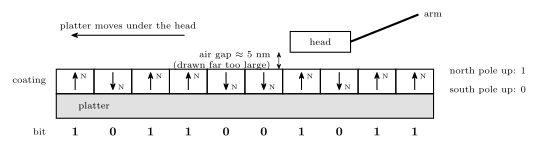
Figure 44: A cross-section along one track, nowhere near to scale. The magnetised coating is divided into tiny patches, and each stores one bit as the direction it is magnetised: north pole up for a 1, south pole up for a 0. The head flies on a cushion of air about 5 nm above the surface and never touches it. As the platter carries the patches past, the head reads each bit by sensing the direction of its field, or writes one by setting it. The underside of the platter has its own coating and its own head; only the top is drawn.
All the heads are mounted on one arm assembly and move in and out together. Only one head reads or writes at a time.
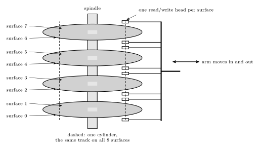
Figure 45: A disk with four platters seen from the side. Each platter has two recording surfaces, so there are eight, numbered 0 to 7 from the bottom, and one read/write head for each. The heads are all on one comb-shaped arm, so they move in and out together: when one head is over a track, every other head is over the track at the same radius on its own surface. Those eight tracks, outlined by the dashed cylinder, form one cylinder.
Tracks, sectors and cylinders
- A track is one circle of data on one surface, at one radius.
- Each track is divided into fixed-length sectors. A sector is the smallest unit of data: the disk always reads or writes a whole sector at a time, typically 512 bytes (4096 on newer disks).
- A cylinder is the set of tracks at a given radial position, one on each surface.
Cylinders
Because the heads move together, they are always positioned over a whole cylinder. Assuming both sides of every platter are used,
\[\text{tracks per cylinder} = 2 \times \text{number of platters}.\]
The four-platter disk above has \(2 \times 4 = 8\) tracks in each cylinder. Data the disk will need together is best placed in one cylinder: switching between its tracks only means switching heads, electronically, with no arm movement at all.
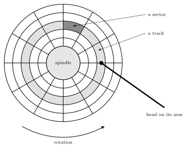
Figure 46: One surface seen from above. The tracks are concentric circles, and each is divided into sectors, here twelve to a track, which are the smallest units the disk reads or writes. The highlighted ring is one track and the dark patch one sector of it. The head sits on its arm over one track at a time, here the highlighted one; the platter turns beneath it, carrying each sector of that track past in turn. The same track on every surface makes up a cylinder.
What a sector holds
A sector is more than its data. Along the track it is laid out as:
- Preamble: a known pattern that lets the head synchronise to the data, finding where the sector starts and the timing of its bits.
- Data: the sector’s payload, typically 512 bytes.
- Error correction code (ECC): extra bits computed from the data that let small read errors be detected and corrected.
- Inter-sector gap: blank space before the next sector’s preamble, a margin for the head and for small speed variations.
The layout follows the same idea as a UART frame (serial-communication): there is no separate clock on the wire or the platter, so something has to announce the start and fix the timing (the start bit; the preamble), the data follows, some redundancy checks it (the parity bit; the much stronger ECC), and a guaranteed idle stretch separates one unit from the next (the stop bits; the gap).
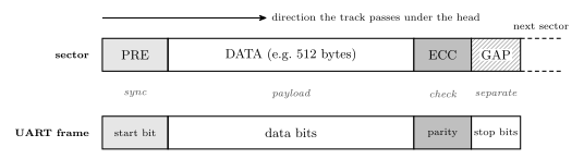
Figure 47: The format of a sector along a track, with a UART frame beneath it for comparison. The preamble lets the head lock on to the timing, the data is the payload, the error-correcting code lets damaged bits be repaired, and the gap separates this sector from the next. A UART frame solves the same problem of sending self-timed data with no clock line, with a start bit, data bits, a parity bit and stop bits; the sector’s ECC is far stronger than parity, which can only detect a single flipped bit.
How much of a disk holds data
The preambles, ECCs and gaps take space on every sector, and the file system’s own tables take more:
- about 85 % of the raw disk capacity is usable by the operating system; the rest is sector overhead;
- about 95 % of that is usable for user data; the remaining ~5 % is file-system overhead (file-systems).
So user data gets about \(0.85 \times 0.95 = 0.8075\), roughly 81 % of the raw capacity, and the file system takes \(0.85 \times 0.05 = 4.25\,\%\) of it.
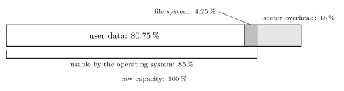
Figure 48: Where a disk’s raw capacity goes. About 15 per cent is spent on each sector’s preamble, error-correcting code and gap, leaving 85 per cent that the operating system can use. The file system’s tables take about 5 per cent of that, 4.25 per cent of the raw capacity, leaving roughly 81 per cent for the files themselves.
Access time
Reading a sector takes three steps, one after another, so
\[\text{access time} = \text{seek time} + \text{rotational latency} + \text{transfer time}.\]
- Seek time: the time to move the heads to the right cylinder. It depends on how far the arm has to travel.
- Rotational latency: the time spent waiting for the sector to arrive under the head, once the head is on the right track. It depends on where the sector happened to be when the head arrived.
- Transfer time: the time for the sector to pass under the head while it is read. One sector is a small fraction of a track, so this is negligible compared with the other two.
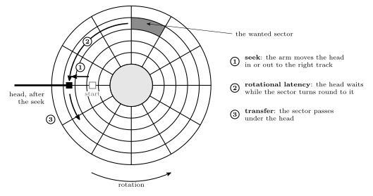
Figure 49: Where the three parts of an access come from, on one surface. The head starts over the wrong track. First the arm moves it in or out to the track that holds the wanted sector (1, the seek). The head is then over the right track, but the sector is somewhere else on the circle, so the head waits while the platter turns the sector round to it (2, the rotational latency): anything from no time to a whole turn, half a turn on average. Then the sector passes under the head as it is read (3, the transfer), a small fraction of a turn. The seek is a movement of the arm and the latency a movement of the platter, and the second cannot start being useful until the first has finished, so the times add.
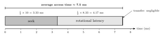
Figure 50: The three parts of a disk access in time order, drawn to scale for the average access of a 7200 rpm disk with a 10 ms edge-to-edge seek. First the arm moves to the right cylinder, 3.33 ms on average; then the head waits for the sector to come round, half a rotation, 4.17 ms on average; then the sector passes under the head, which takes only microseconds and is too thin to see at this scale. Both of the large parts are mechanical, which is why a disk is thousands of times slower than main memory.
Average rotational latency
Let \(T\) be the time for one rotation. When the head arrives on the track, the wanted sector may be just arriving (wait 0) or may have just gone past (wait almost \(T\)), and every position in between is equally likely. The average of a wait spread evenly between 0 and \(T\) is the midpoint,
\[\text{average rotational latency} = \frac{T + 0}{2} = \frac{T}{2},\]
half a rotation.
Average seek time
The edge-to-edge seek time is the time to move from the outermost cylinder to the innermost, the longest possible seek. If seek time is proportional to the number of tracks crossed, the average seek depends on the average distance between where the heads are and where they need to go.
Measure positions as a fraction of the way across the disk, from 0 at one edge to 1 at the other. Take the starting position \(x\) and the target \(y\) as independent and both uniformly random. The distance is \(|x - y|\), and its average is
\[\int_0^1\!\!\int_0^1 |x - y|\,dx\,dy = 2\int_0^1\!\!\int_0^x (x - y)\,dy\,dx = 2\int_0^1 \frac{x^2}{2}\,dx = \frac13.\]
The factor 2 is the symmetry: the region \(y > x\) contributes the same as \(y < x\). So
\[\text{average seek time} = \frac13 \times \text{edge-to-edge seek time}.\]
It is not one half. Half would be right if the heads always started at one edge, but the start is random too. Two random points on a line are on average a third of its length apart: short seeks are much commoner than long ones, because a long seek needs both ends near opposite edges.
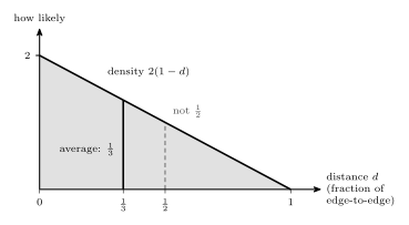
Figure 51: Why the average seek is a third of the edge-to-edge seek. If the start and the target are independent and each uniform across the disk, the distance d between them has density 2(1 - d): short seeks are common and a full edge-to-edge seek is rare, because it needs both ends at opposite edges. The balance point of that triangle is at d = 1/3, not 1/2. One half would be the average only if every seek began at an edge.
Worked: average access time of a 7200 rpm disk
What is the average access time for a hard disk which rotates at 7200 rpm and has an edge-to-edge seek time of 10 ms? Assume that seek time is proportional to the number of tracks to seek.
The rotation period. \(7200\) revolutions per minute is
\[\frac{7200}{60} = 120 \text{ revolutions per second}, \qquad T = \frac{1}{120}\text{ s} = \frac{1000}{120}\text{ ms} = 8.33\text{ ms}.\]
Average seek. Seek time is proportional to distance, so the average seek is a third of the edge-to-edge time: \(\frac13 \times 10 = 3.33\) ms.
Average rotational latency. Half a rotation: \(\frac12 \times 8.33 = 4.17\) ms.
Transfer time. Negligible. As a check, if a track held 1000 sectors, one sector would pass in \(8.33\text{ ms} / 1000 = 8.3\ \mu\)s, under 0.2 % of the total.
Total.
\[\text{average access time} = \frac13(10\text{ ms}) + \frac12\left(\frac{1000}{120}\text{ ms}\right) + \text{negligible} = 3.33 + 4.17 = \mathbf{7.5\ ms}.\]
The convention matters. Taking the average seek as half the edge-to-edge time would give \(5 + 4.17 = 9.17\) ms. These notes use one third, because the question says seek time is proportional to the tracks crossed and both the start and the target position are random, and for that the average distance is exactly a third of the way across (Figure 51). Half is the average only for seeks that start from one edge.
A faster disk. At 10,000 rpm, \(T = 60/10{,}000\) s \(= 6\) ms, the average latency is 3 ms, and with the same seek the average access time is \(3.33 + 3 = 6.33\) ms. Spinning faster only shortens the latency; the seek is the arm’s job.
Common mistakes
- Using the full rotation as the latency. On average the sector is half a turn away: \(T/2\), not \(T\).
- Using half the edge-to-edge seek as the average. With random start and end positions the average distance is a third of the way across, so the average seek is a third of the edge-to-edge time.
- Forgetting to convert rpm. Divide by 60 for revolutions per second, then invert for the period, then multiply by 1000 for milliseconds: 7200 rpm is 8.33 ms per turn.
- Counting a cylinder’s tracks as the number of platters. Each platter has two surfaces, so a cylinder has \(2 \times\) platters tracks.
- Thinking a disk can read part of a sector. The sector is the smallest unit read or written; changing one byte means rewriting the whole sector.
- Taking the raw capacity as space for files. About 85 % is usable by the operating system, and about 95 % of that by files.
See also
- memory-hierarchy-and-cache — disks among the other levels of memory
- file-systems — how sectors are grouped into blocks and files, and why fragmentation hurts the access time
- memory-technologies — SSDs, the flash-based alternative with no moving parts
- serial-communication — the UART frame, the same start, data, check and stop idea
- 2026-10-22-memory-disks-and-files — Lecture 24
Memory Hierarchy and Cache
Why a computer has several layers of memory rather than one, and how a cache makes a slow main memory look fast. This note covers the memory hierarchy from registers down to tape, how speed, capacity and cost per bit change from one level to the next, what a cache is and why it works, the three cache levels, and the average access time with a cache. The technologies at each level are in memory-technologies, and the disk level in magnetic-disks. First met in 2026-10-22-memory-disks-and-files.
The memory hierarchy
No single memory is fast, large and cheap at once. Fast memory costs more per bit, so it is built small. Cheap memory is slow, so it is built large. A computer therefore stacks several kinds, with the fastest and smallest next to the processor and the largest and cheapest furthest away.
| Level | Built from | Typical capacity | Cost per bit | Access time, order of magnitude |
|---|---|---|---|---|
| Registers (r0 to r31 on the AVR) | flip-flops, inside the CPU | under a kB | highest | ~1 ns |
| Cache (L1, L2, L3) | SRAM | ~MB | high | ~10 ns |
| Main memory | DRAM | ~GB | moderate | up to ~1 µs |
| Magnetic disk (and SSD) | magnetic platters, or flash | ~TB | low | ~1 to 10 ms |
| Tape, optical disk | magnetic tape, optical discs | ~PB, across a library of them | lowest | ~100 ms and up; a tape that must wind takes seconds |
Going down the hierarchy:
- capacity grows, from bytes to petabytes;
- cost per bit falls, from the most expensive to the cheapest;
- access time grows, by roughly a factor of 10 to 1000 per level.
The CPU works directly only with the top. Data moves up the levels as it is needed and back down when it is not.
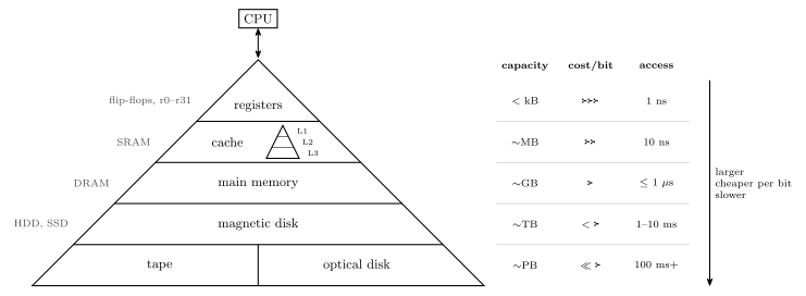
Figure 52: The memory hierarchy, with the CPU at the apex. Each level is larger, cheaper per bit and slower than the one above it: registers are under a kilobyte and answer in about a nanosecond, while a tape or optical library holds petabytes and takes a tenth of a second or more. The width of each band suggests its capacity. The cache is itself a small hierarchy of three levels, L1 to L3, drawn as a pyramid within its band. The figures on the right are orders of magnitude, not specifications.
Cache memory
CPUs are faster than main memory. A processor can execute an instruction in well under a nanosecond, while DRAM takes tens to hundreds of nanoseconds or more to answer. Memory as fast as the CPU exists (SRAM), but very fast memory is expensive, so it cannot be the whole of main memory. If the CPU always had to wait for main memory, performance would suffer badly: most of its time would be spent idle.
A cache is the compromise: a small amount of very fast memory combined with the larger, slower main memory. The most commonly used memory words are kept in the cache. On every access the CPU looks in the cache first:
- if the word is there, a hit, it is returned at cache speed;
- if not, a miss, it is fetched from main memory over the bus, and a copy is kept in the cache in case it is wanted again.
The average access time is greatly reduced if many words are found in the cache.
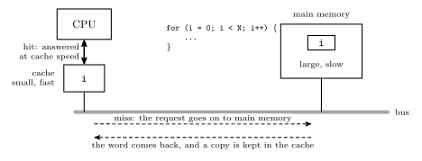
Figure 53: A cache between the CPU and the bus. The CPU asks the cache first; only on a miss does the request travel along the bus to the much slower main memory. A loop counter i is the typical resident: the first read of i misses and brings a copy into the cache, and every later read of it, once per iteration, is a hit that never touches the bus.
Why a cache works
A cache only helps if the words a program uses next are mostly the ones it used recently. They are, because programs are repetitive:
- The same data is used again soon. A loop such as
for (i = 0; i < N; i++) { ... }reads and writesion every iteration. If the loop runs \(10^{20}\) times,iis accessed at least \(10^{20}\) times; only the first of those can miss. Variables in use, the top of the stack, and the loop’s own instructions all behave like this. - Neighbouring data is used soon after. Instructions are fetched in sequence, and arrays are walked element by element. A cache fetches a small block of neighbouring words on a miss, so the next few accesses hit.
The first is called temporal locality and the second spatial locality. Together they mean that a cache holding a tiny fraction of main memory can still answer the large majority of accesses.
Cache levels
There are often several levels of cache, each larger and slower than the one before:
| Level | Where | Typical size | Speed |
|---|---|---|---|
| L1 | inside the CPU itself | 32 kB to 128 kB | runs at the same speed as the CPU |
| L2 | a separate chip (possibly in the same module), or on the same chip as the CPU | 256 kB to 16 MB | may be slightly slower than the CPU |
| L3 | on some machines, a third level, usually shared by all the cores | 2 MB to 256 MB | slower again, still much faster than DRAM |
The CPU looks in L1, then L2, then L3, and only then in main memory. The cache is a hierarchy within the hierarchy. Sizes here are in bytes: B is a byte and b is a bit, so 32 kB is \(32 \times 1024 \times 8 = 262{,}144\) bits.
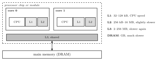
Figure 54: Three levels of cache between the CPU core and main memory. L1 sits inside the core and keeps up with it; L2 is larger and may be slightly slower; L3, on machines that have it, is larger still and usually shared by every core on the chip. A request falls through the levels in order and goes out to DRAM only if all three miss. Each level is roughly ten times the size of the one above it.
Average access time with a cache
Let the cache take \(t_c\), main memory \(t_m\), and let \(h\) be the hit rate, the fraction of accesses found in the cache. The CPU looks in the cache first, so every access pays \(t_c\), and the fraction \(1 - h\) that miss pay \(t_m\) as well:
\[t_{\text{avg}} = t_c + (1 - h)\, t_m.\]
The same thing weighted hit by miss: a hit costs \(t_c\) and a miss \(t_c + t_m\), so \(t_{\text{avg}} = h\,t_c + (1-h)(t_c + t_m)\), which expands to the line above.
If the cache and main memory are searched at the same time instead, a miss costs only \(t_m\) and \(t_{\text{avg}} = h\,t_c + (1-h)\,t_m\). The two differ by \(h\,t_c\), which is small whenever \(t_c \ll t_m\); the first form is used below.
Worked: how much a cache saves
A cache answers in 10 ns and main memory in 1 µs. What is the average access time with no cache, and with a cache whose hit rate is 90 %, 95 % and 99 %?
No cache. Every access goes to main memory: 1000 ns.
With the cache, \(t_{\text{avg}} = 10 + (1 - h) \times 1000\) ns:
| Hit rate \(h\) | Misses | \(t_{\text{avg}}\) | Faster than no cache by |
|---|---|---|---|
| 90 % | 1 in 10 | \(10 + 0.10 \times 1000 = \mathbf{110}\) ns | 9.1 times |
| 95 % | 1 in 20 | \(10 + 0.05 \times 1000 = \mathbf{60}\) ns | 16.7 times |
| 99 % | 1 in 100 | \(10 + 0.01 \times 1000 = \mathbf{20}\) ns | 50 times |
Two things to notice. The misses dominate: at 95 % the cache contributes 10 ns and the misses 50 ns. And every extra per cent of hit rate near the top is worth a lot, which is why caches are made as large as cost allows and stacked in levels. For the loop above, reading i a thousand times with one miss gives \(h = 0.999\) and \(t_{\text{avg}} = 10 + 0.001 \times 1000 = 11\) ns, close to the speed of the cache itself.
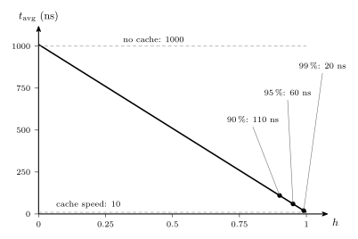
Figure 55: Average access time against hit rate, for a 10 ns cache in front of a 1 µs main memory. With no hits every access costs the full microsecond plus the wasted look in the cache; as the hit rate rises the average falls in a straight line towards the cache’s own 10 ns. The marked points are the worked hit rates: 90, 95 and 99 per cent give 110, 60 and 20 ns. Most of the benefit arrives only at high hit rates, where the line approaches the cache speed.
Common mistakes
- Reading the hierarchy as “faster is better, so use only the top”. The top is fast precisely because it is small and expensive. The hierarchy exists because no level can do every job.
- Forgetting the lookup cost on a miss. With a look-in-the-cache-first design, a miss costs \(t_c + t_m\), not \(t_m\).
- Weighting by the wrong fraction. \(1 - h\) multiplies the main-memory time; a 95 % hit rate means 5 % of accesses go to main memory.
- Mixing B and b. Cache sizes are in bytes: 32 kB of L1 is 256 kibibits.
- Thinking a cache adds capacity. A cache holds copies of words that are also in main memory. It makes memory faster, not larger.
See also
- memory-technologies — SRAM, DRAM and the rest of the memories at each level
- magnetic-disks — the disk level, and why its access time is in milliseconds
- file-systems — how the bottom levels are organised into files
- cpu-organisation · fetch-decode-execute-cycle — the CPU at the top of the hierarchy and how often it reaches into memory
- avr-architecture — a machine with no cache: the AVR’s SRAM already runs at CPU speed
- 2026-10-22-memory-disks-and-files — Lecture 24
Memory Models
The first of the four things that make up an ISA (instruction-set-architecture): how memory looks to the CPU. Four issues decide that — addressable cell size, alignment, address spaces and endianness — and every one of them is a decision the specification has to make, not something the hardware settles on its own.
Memory as addressable cells
Computer memory is conceptually a set of addressable cells:
- Each cell has a unique address (or cell number).
- Cells are usually 8 bits wide (i.e. hold one byte).
- Various cell widths have been used in the past — 8 bits is a convention, not a law.
Drawn as a table, the address indexes the rows and the cell width is how wide each row is:
| Address | ← cell width → |
|---|---|
| 0 | |
| 1 | |
| 2 | |
| 3 | |
| … |
A “4 × 3 memory” in that notation means 4 addresses of 3-bit cells — and \(4 = 2^2\), so two address bits. Built at gate level, it shows that “memory” at this level is nothing more exotic than flip-flops-and-latches and combinational-logic-blocks arranged into storage.
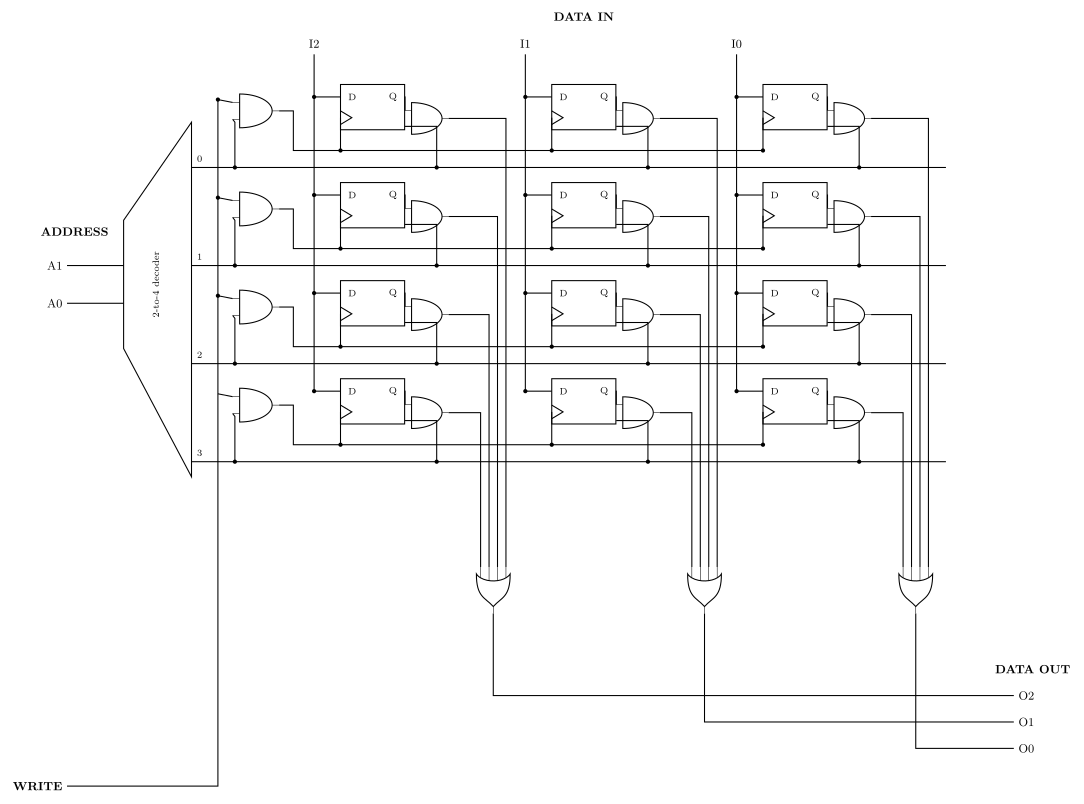
Figure 56: A 4 × 3 memory at gate level — four addresses of three-bit cells. Twelve D flip-flops in four rows of three: one row is one addressable cell. The decoder turns A1 A0 into exactly one row-select (word) line. Writing: the word line ANDed with WRITE clocks that row’s three flip-flops, so DATA IN (I2 I1 I0) — which is wired to every row’s D inputs all the time — is captured only by the selected row. Reading: each flip-flop’s Q is ANDed with its own word line and the three cells of a column are OR’d together, so the unselected rows contribute 0 and DATA OUT (O2 O1 O0) carries the selected row alone. The decoder is drawn as a trapezoid with the wide edge on the right, and the flip-flops as plain rectangles with a clock wedge on the lower-left edge, per this course’s conventions (csse2010-diagram-notation). The most significant bit, I2/O2, is the leftmost column.
A. Addressable cell size
Most common cell size is 8 bits (1 byte) — but not always.
The AVR is the counterexample sitting on the bench:
| AVR memory | Cell width |
|---|---|
| Data memory | 8 bits |
| Instruction (program) memory | 16 bits |
Which is why an AVR instruction is “one word” rather than “two bytes” — a program-memory address counts 16-bit cells.
The bus transports the content of a cell, but the data bus may be wider than one cell: it can retrieve several cells (addresses) at once. When it does, the address bus does not need to be as wide.
Bus sizes
For every doubling of the data bus width, remove the least significant bit of the address bus.
For a memory of \(2^n\) cells at 8 bits per cell — so an address size of \(n\) bits:
| Data bus | Address bus | Cells per transfer |
|---|---|---|
| 8 bits | \(n\) bits | one cell at a time |
| 16 bits | \(n-1\) bits | two cells at a time |
| 32 bits | \(n-2\) bits | four cells at a time |
The reason is that a wide transfer always moves an aligned group of cells. With a 16-bit data bus the memory only ever hands over cell pairs \((0,1), (2,3), (4,5), \dots\) — so the bottom address bit never selects anything, and naming the pair takes one bit fewer than naming the cell.
Worked example. A memory of 64 cells, 8 bits each, addressed 000000 … 111111:
\[64 = 2^6 \text{ cells} \implies 6\text{-bit addresses}\]
| Data bus | Address bus |
|---|---|
| 8 | 6 |
| 16 | 5 |
| 32 | 4 |
Read the two buses as a pair, not separately: widening one narrows the other by exactly as much.
Word addresses and byte addresses
The AVR’s 16-bit program-memory cells have one practical consequence. The program counter, jmp, call and every code label count words. But a table of constant bytes kept in flash is read a byte at a time by lpm, load program memory, and lpm takes a byte address in the Z register. Word \(w\) holds bytes \(2w\) and \(2w + 1\), with the low byte at the even address, which is the AVR being little endian (section D).
So turning a code label into a byte address means doubling it. Take the string Hello stored at word 2 by mesg: .db 72,101,108,108,111 (assembly-process):
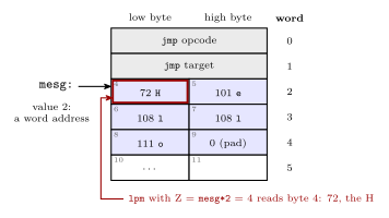
Figure 57: One region of program memory addressed two ways. Each row is a 16-bit word, numbered on the right, and each half is a byte, numbered inside its cell. The label mesg has the value 2 because labels in the code segment count words. Byte addressing counts the halves, low byte first, so word 2 starts at byte 4. That is why lpm is pointed at mesg*2: with Z = 4 it loads 72, the H. The five bytes of the string take two and a half words, and the last half word is a zero pad. Grey marks the jmp, blue the string and red the byte that lpm reads.
        ldi  ZH, high(mesg*2)   ; Z = 4: byte address of word 2
        ldi  ZL, low(mesg*2)
        lpm                     ; r0 <- 72, the H
Leaving out the *2 points Z at byte 2, the low byte of word 1, which is half of the jmp.
B. Alignment
Many architectures require natural alignment, e.g.
- 4-byte words starting at addresses 0, 4, 8, …
- 8-byte words starting at addresses 0, 8, 16, …
i.e. an \(n\)-byte value must start at an address that is a multiple of \(n\).
Taking an 8-byte word on a machine that fetches 8 bytes at a time:
| Where it sits | Reads needed | |
|---|---|---|
| Aligned | bytes 8–15, i.e. an 8-byte word at address 8 | 1 — it is exactly one fetched block |
| Non-aligned | bytes 12–19, i.e. an 8-byte word at address 12 | 2 — the top half of block 8–15, plus the bottom half of block 16–23 |
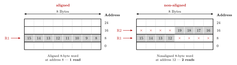
Figure 58: An aligned and a non-aligned 8-byte word. Four blocks of eight bytes; grey marks the bytes of the 8-byte word. On the left the word starts at address 8, so it is one block — one read. On the right it starts at address 12, so it takes the top half of the block at 8 and the bottom half of the block at 16 — two reads, marked R1 and R2. Two things about the drawing: addresses increase upward (unlike every other memory figure in the course, where they increase downward — see csse2010-diagram-notation on that inconsistency), and byte numbers within a row run high-to-low left to right. The × marks a byte in the fetched block that is not part of the word.
Alignment is often required because it is more efficient — the aligned case is always one read, the non-aligned case sometimes two, and the hardware that stitches two blocks together and extracts the middle is hardware that a machine demanding alignment simply does not need.
When alignment is not required — the Pentium IV
- Fetches 8 bytes at a time from memory (64-bit wide data bus).
- Alignment is NOT required, so the processor stays backwards compatible with earlier processors.
- A 4-byte word stored at address 4 takes 1 read (bytes 0 to 7).
- A 4-byte word stored at address 6 must read bytes 0 to 7 (one read) and bytes 8 to 15 (second read), then extract the 4 required bytes from the 16 bytes read.
Counting reads in general
A data bus \(w\) bytes wide delivers one aligned \(w\)-byte block per read. An \(n\)-byte value starting at address \(a\) therefore costs
\[\left\lceil \frac{(a \bmod w) + n}{w} \right\rceil \text{ reads}\]
The best case is \(n/w\) (rounded up), when the value starts on a block boundary; every other starting offset can push it one block further. So a value read from an arbitrary address costs either \(\lceil n/w \rceil\) or one more than that — which is why questions of this shape almost always answer “\(k\) or \(k+1\)” rather than a single number.
Worked example: an 8-byte value on a 16-bit data bus, no natural alignment required. Here \(w = 2\) and \(n = 8\):
| Starting address | Spans | Reads |
|---|---|---|
| Even | 4 aligned 2-byte blocks | 4 |
| Odd | 9 byte-positions, so 5 aligned blocks | 5 |
so the answer is 4 or 5. The odd case is the one to picture: one byte of the value sits alone at the top of the first block and one byte alone at the bottom of the last, and each of those still costs a whole read.
C. Address spaces
Many microprocessors have a single linear memory address space — the von Neumann architecture:
- e.g. \(2^{32}\) bytes numbered from 0 to \(2^{32} - 1\).
- (These may not be bytes — it depends on the addressable cell size.)
- Program and data share the one space.
However, the Harvard architecture has separate address spaces for instructions and data. The same numeric address means a different location depending on which space you are in, and an instruction says which one it means by what instruction it is.
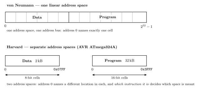
Figure 59: The two address-space models. Above: von Neumann — one linear space, so program and data are separated only by convention and address 0 names exactly one cell. Below: Harvard, in the AVR ATmega324A’s shape — two spaces, each starting at its own 0, with different sizes and different cell widths — and the cell width under each box is the whole reason the arithmetic below works out the way it does: 32 kB of program memory is \(2^{15}\) bytes but only \(2^{14}\) addresses, because each address there names a 16-bit cell. The end addresses follow from the sizes, so the data box ends at 0x07FF (\(2^{11}-1\), for 2048 bytes) rather than the 0x08FF of Figure 60, which is that 2 kB plus the 256 locations in front of it.
AVR ATmega324A is Harvard:
| Space | Size | Address width |
|---|---|---|
| Data | \(2^{11}\) (2048) bytes | 11 bits |
| Instruction | \(2^{14}\) 16-bit words — 16,384 instruction words = 32,768 bytes | 14 bits |
The arithmetic — convert to cells first, then take the logarithm:
\[\text{data: } 2\,\text{kB} = 2 \cdot 2^{10}\,\text{B} = 2^{11} \text{ cells (8-bit)} \implies 11 \text{ bits}\] \[\text{program: } 32\,\text{kB} = 2^{5} \cdot 2^{10}\,\text{B} = 2^{15}\,\text{B} = 2^{14} \text{ cells (16-bit)} \implies 14 \text{ bits}\]
The program-memory step is the one that catches people: 32 kB of flash is only \(2^{14}\) addresses, not \(2^{15}\), because each address names a 16-bit cell. Halve the byte count before taking the log whenever the cells are not bytes.
Laid out as a memory map (see avr-architecture for the rest of the chip):
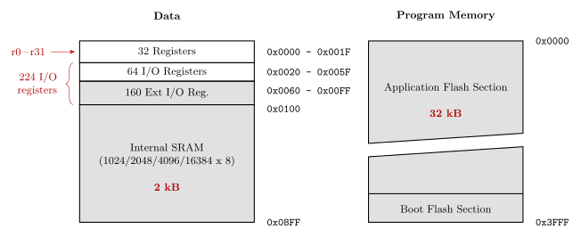
Figure 60: The ATmega324A’s two address spaces. Lowest address at the top, hex addresses outside on the right, grey fill on the coarsely-described regions, and the diagonal break across the flash meaning not to scale: that is this course’s memory-map convention (csse2010-diagram-notation). Marked in red: the register file is r0–r31, the 64 I/O plus 160 extended I/O registers are the 224 of avr-io-ports, the SRAM is 2 kB and the flash 32 kB.
Two details worth pinning down. 0x3FFF \(= 2^{14} - 1\), which is the 14 bits above. And the data space runs to 0x08FF — that is the 2 kB of SRAM plus the 256 locations (0x0000–0x00FF) that the register file and I/O registers occupy in front of it; the “\(2^{11}\) bytes” above is the SRAM itself, which is what the 11 bits size.
The assembler’s view: segments
An assembler treats each address space as a segment with its own location counter (assembly-process). On the ATmega324A there are three, because the EEPROM is a third address space alongside the two above:
| Segment | Directive | Address space | Cell | Counter starts at | The assembler can |
|---|---|---|---|---|---|
| code | .cseg |
program memory, flash, 32 kB | 16-bit word | 0x0000 |
place instructions and constants |
| data | .dseg |
data memory, SRAM | byte | 0x0100 |
only reserve space |
| EEPROM | .eseg |
EEPROM, 1 kB | byte | 0x0000 |
place constants |
Three consequences of separate spaces:
- The same number means different places. Address 0 is the reset
jmpin the code segment, registerr0in data memory and the first EEPROM byte in the EEPROM segment. - The units differ.
.org 0x0100in the code segment is word 256, which is bytes 512 and 513 of flash. In the data segment it is byte0x0100. - The data counter does not start at 0. The first 256 data addresses are the registers and I/O registers of Figure 60, so the first variable lands at
0x0100.
The data segment can only be reserved, not filled, because the assembler’s output is programmed into flash and EEPROM, which keep their contents, while SRAM starts empty at every power-up.
The memory behind each space
The three spaces are three different kinds of memory, and the kind explains how each is used (memory-technologies):
| Space | Technology | Volatile? | Erased and rewritten |
|---|---|---|---|
| Program memory | flash | no | electrically, a block at a time |
| Data memory | SRAM, flip-flops | yes | written a byte at a time, freely |
| EEPROM | EEPROM | no | electrically, one cell (byte) at a time |
The flash is divided into two blocks, the Application Flash Section and the Boot Flash Section of Figure 60. Because flash is erased a block at a time, a boot loader in the boot section can erase and rewrite the application section without erasing itself. Other AVR devices have one flash block, and some have more.
The register file and the SRAM sit at the top of the memory hierarchy. Unlike a desktop processor, the AVR has no cache: its SRAM is small enough and fast enough to keep up with the CPU directly.
D. Endianness
Different machines may support different byte orderings for a multi-byte value.
| Which end goes first (at the lowest address) | Used by | |
|---|---|---|
| Little endian | the little end — least significant byte | Intel microprocessors (Pentium etc.), and AVR |
| Big endian | the big end — most significant byte | SPARC, Freescale (formerly Motorola) microprocessors |
Most desktop/workstation/server CPUs produced since ~1992 are “bi-endian” (support both) — some switchable at boot time, others at run time, i.e. they can change dynamically.
Endianness only ever matters when a value spans more than one cell: reassembling it means knowing which cell was the low-order one.
Worked example
Given this memory:
| Address | Contents |
|---|---|
| 0 | 00001111 |
| 1 | 00110011 |
| 2 | 11011101 |
| 3 | 00101100 |
| Read | Value | Why |
|---|---|---|
| the 1-byte word at address 1 | 00110011 |
one cell — endianness does not apply |
| the 2-byte word at address 0, big endian | 00001111 00110011 |
big end first, so address 0 holds the most significant byte |
| the 2-byte word at address 2, little endian | 00101100 11011101 |
little end first, so address 2 holds the least significant byte and address 3 the most |
The mechanical way to do these without getting turned around: write the addresses the value occupies in increasing order, then assemble the answer most-significant-byte first. Big endian reads the addresses forwards; little endian reads them backwards.
See also
- instruction-set-architecture — the four pillars this is the first of
- avr-architecture — the ATmega324A’s two address spaces in full
- addressing-modes — how an instruction names a memory location
- binary-number-representations · flip-flops-and-latches · combinational-logic-blocks
- assembly-process — segments, location counters, and
.dbpacking two bytes to a word - compilation-and-linking — where a C compiler puts globals, locals and the heap in data memory
- memory-technologies — flash, SRAM and EEPROM as technologies, and why sizes are powers of 2
- memory-hierarchy-and-cache — registers, cache, main memory and disk, by speed and cost
- 2026-08-31-instruction-set-architecture-part-1 — Lecture 11 · 2026-10-08-assembly-process — Lecture 20 · 2026-10-22-memory-disks-and-files — Lecture 24
Memory Technologies
The kinds of memory a computer is built from, and how big they are. This note covers why a computer needs memory at all, the five ways memory is classified and where SRAM, DRAM, ROM, flash, SSDs and hard disks fall on each, how a static cell differs from a dynamic one, what “RAM” means now, the ROM family from ROM to flash, the ATmega324A’s three memories, the generations of DRAM, and the units capacity is quoted in, where “1 MB” can mean three different numbers. How these memories are arranged by speed is in memory-hierarchy-and-cache, and disks and files are in magnetic-disks and file-systems. First met in 2026-10-22-memory-disks-and-files.
Why a computer needs memory
A processor on its own holds a few dozen registers. Everything else has to live somewhere, and there are three distinct jobs:
- Temporary results. Intermediate values, variables, the stack: things a running program needs for a while and then discards.
- Programs. The instructions themselves have to be stored somewhere the processor can fetch them from (fetch-decode-execute-cycle).
- Settings that survive power-off. A calibration constant, a high score, the last channel a TV was on. These must still be there when the power comes back.
The first job wants memory that is fast and can be rewritten endlessly. The third wants memory that keeps its contents with no power. No single technology is best at all three, which is why there are many types.
Five ways to classify memory
Each axis asks one question about a memory.
| Axis | The question | The two answers |
|---|---|---|
| Access | Can any cell be reached directly, in the same time? | random access: the address selects the cell directly. Sequential access: the data has to be passed over in order to reach a cell, like a tape |
| Static or dynamic | Does a stored bit stay put by itself while powered? | static: held by a flip-flop or latch. Dynamic: held as charge that leaks away and must be refreshed |
| Volatility | Does it keep its contents when the power is off? | volatile: forgets. Non-volatile: remembers |
| Read-only | Can the processor write it in normal use? | read/write, or read-only (written once, or only by a special process) |
| Primary or secondary | Does the processor address it directly? | primary: on the processor’s address bus, holding the running program and its data. Secondary: reached through I/O, holding files |
Random access is what an address decoder gives you. In the gate-level memory of memory-models, the address bits drive a decoder that selects exactly one row, and it takes the same time whichever row it is. A tape has to wind past everything in front of the data first.
Where the common technologies fall:
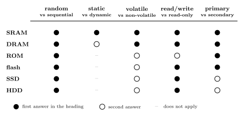
Figure 61: Six memory technologies against the five ways of classifying memory. Each row is one technology and each column one axis; a filled dot means the left-hand answer in the column heading, an open circle the right-hand one. SRAM and DRAM are both random-access, volatile, read/write primary memory, and differ only in being static or dynamic. ROM and flash are non-volatile; ROM is read-only, while flash is rewritten electrically, in blocks. SSDs (built from flash) and hard disks are secondary storage, reached through I/O rather than the address bus. All six are random access, in that any location can be reached directly by its address; the sequential case is tape. A hard disk’s access time does still depend on where the data is, because it must wait for the head to move and the disk to turn. The static/dynamic distinction only applies to the semiconductor RAMs, so it is left blank for the rest.
Two entries need a word. Flash is used both as primary memory (the program memory of a microcontroller like the AVR, which the processor fetches instructions from directly) and, packaged as an SSD, as secondary storage. And a hard disk counts as random access (sometimes called direct access) because the head can go straight to any track without reading what lies in between, unlike a tape. Reaching a sector still means moving the head and waiting for the sector to rotate underneath, though, so unlike a memory chip its access time depends on where the data is (magnetic-disks).
Static and dynamic memory
Static memory (SRAM) stores each bit in a flip-flop or latch: a loop of gates that holds its state for as long as the power is on (flip-flops-and-latches). Nothing needs doing to keep the bit. A typical cell is two cross-coupled inverters plus two switches to connect it to the bit lines, about six transistors per bit, so SRAM is fast but expensive per bit.
Dynamic memory (DRAM) stores each bit as charge on a capacitor, with a transistor as a switch that connects the capacitor to its bit line when the row is selected. One transistor and one capacitor per bit is far smaller than a flip-flop, so many more bits fit on a chip and each costs less. The price is that the charge leaks away. A DRAM cell forgets its contents within milliseconds unless it is refreshed, meaning read and written back, which the memory does to every row every few tens of milliseconds (of the order of 20 ms). Reading is slower too, because the small charge has to be sensed and amplified.
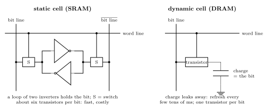
Figure 62: One bit of static and one bit of dynamic memory. Left: the static cell is two inverters in a loop. Whatever value sits at one side, the other inverter feeds its complement back, so the pair holds the bit for as long as there is power. Raising the word line closes both switches and connects the two sides to the bit line and its complement, for reading or writing. Right: the dynamic cell is a single switch (a transistor) and a capacitor. Raising the word line connects the capacitor to the bit line; a charged capacitor is a 1 and an empty one a 0. The charge leaks away through the switch, so the cell has to be read and rewritten, refreshed, every few tens of milliseconds.
| SRAM | DRAM | |
|---|---|---|
| Bit stored in | a flip-flop or latch | charge on a capacitor, behind a transistor switch |
| Keeps its bit while powered? | yes | only if refreshed every few tens of ms |
| Cell size | large (about six transistors) | small (one transistor, one capacitor) |
| Bits per chip | fewer | many more |
| Speed | faster | slower |
| Cost per bit | high | low |
| Volatile? | yes | yes |
| Typical use | registers, cache, small microcontroller RAM (the ATmega324A’s 2 kB) | a computer’s main memory |
What “RAM” means
RAM stands for random access memory. Originally that meant exactly the first axis above: any cell can be accessed directly, as opposed to sequential access. By that definition ROM and flash are random access too.
In current use “RAM” means volatile read/write memory, and SRAM and DRAM are the two kinds. So “RAM” and “ROM” are treated as opposites even though the original meaning of RAM covers both.
Volatile and non-volatile memory
Volatile memory forgets its contents when the power goes off. Both SRAM and DRAM are volatile. DRAM is volatile even with the power on, in the sense that it forgets within milliseconds if it is not refreshed.
Non-volatile memory remembers its contents with the power off. There are several kinds, and they differ in how, and how easily, they can be rewritten. Hard disks and optical disks are non-volatile too, but they are secondary storage; the next section is about non-volatile chips.
From ROM to flash
- ROM, read-only memory. The contents are hardwired into the silicon by the chip’s manufacturer. They can never be changed.
- EPROM, erasable programmable ROM. Programmed electrically by the user, and erased by ultraviolet light. An EPROM package has a small quartz window over the die. Shining a UV lamp through it for some minutes erases the whole chip, which can then be programmed again.
- EEPROM, electrically erasable PROM. Erased by applying a certain voltage, so it can be erased and rewritten in the circuit, with no lamp, one cell (byte) at a time.
- Flash. A newer form of EEPROM. The two used to be different technologies and have been converging. The main difference that remains is that flash is written and erased in blocks, where EEPROM is written and erased one cell at a time. Erasing a large block at once is what makes flash dense and cheap, and it is why flash holds programs and files while EEPROM holds a few bytes of settings that change one at a time.
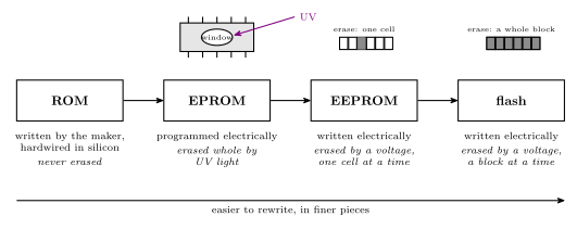
Figure 63: The family of non-volatile memory chips, from least to most easily rewritten. Each step keeps the contents with the power off and changes how they are erased. ROM cannot be erased at all: the bits are fixed when the chip is made. An EPROM is erased whole, by ultraviolet light shining through a window in the package. An EEPROM is erased electrically, in the circuit, a single cell at a time. Flash is erased electrically too, but a block of many cells at a time, which is what lets it be so dense.
The ATmega324A’s three memories
The ATmega324A has one of each of the three common kinds on the chip, and each is a separate address space with its own assembler segment (memory-models, assembly-process).
| Memory | Technology | Size | Holds | Volatile? | Assembler segment |
|---|---|---|---|---|---|
| Flash | flash (block-erased EEPROM) | 32 kB, as 16-bit words | the program and constant tables | no | .cseg |
| SRAM | static RAM | 2 kB | variables, the stack, the heap | yes | .dseg |
| EEPROM | EEPROM (cell-erased) | 1 kB | settings that must survive power-off | no | .eseg |
The flash is divided into two blocks: an application section, where the program normally lives, and a boot loader section at the top of program memory. A boot loader is a small program that can receive a new program, over a serial link for instance, and write it into the application section. Because flash is erased a block at a time, having the program in a separate block from the boot loader means the application can be erased and rewritten while the boot loader that is doing the rewriting stays intact. Other AVR devices have one flash block, and some have more.
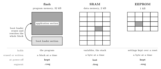
Figure 64: The ATmega324A’s three memories as technologies: what each holds, the unit it is erased or written in (dark), and whether it survives power-off. Flash holds the program and keeps it with the power off, but it can only be erased a block at a time, so it is split into two blocks: a boot loader in the small block can erase and rewrite the program in the large one without erasing itself. SRAM holds the variables and the stack; any byte can be written at any time, at full speed, but all of it is lost at power-off. EEPROM keeps its bytes with the power off and, unlike flash, erases and rewrites them one at a time, which suits a few settings that change one by one.
The table is the answer to a common question: which memory should this value go in? Code goes in flash. A variable the program changes goes in SRAM. A value the program changes and that must still be there after a reset goes in EEPROM.
Generations of DRAM
Every DRAM stores bits as charge on a capacitor, not in flip-flops. Its cells are smaller than a static cell, so a chip packs in more bits, and it is slower than static memory. What has changed over the generations is the interface, the way rows and columns are addressed and data is moved out:
| Generation | What it changed |
|---|---|
| FPM DRAM, fast page mode | once a row is open, further columns in that row can be read without re-sending the row |
| EDO DRAM, extended data out | keeps the output valid while the next column address is sent, so successive reads overlap; a refinement of FPM |
| SDRAM, synchronous DRAM | runs from a clock shared with the memory controller, so transfers happen on clock edges and can be pipelined |
| RDRAM, Rambus DRAM | a narrow, very fast proprietary bus |
| DDR SDRAM, double data rate, generations 1 to 5 | transfers data on both the rising and falling clock edges; each generation raises the rate |
| GDDR, graphics DDR, up to GDDR7 | a DDR variant tuned for the bandwidth of graphics cards |
FPM and EDO belong together as the asynchronous generations. SDRAM is the break: from there on, DRAM is clocked, and DDR4 and DDR5 are what current machines use.
Capacity units: powers of 2 or of 10
In SI units, kilo, mega and giga mean powers of 10: \(10^3\), \(10^6\), \(10^9\). In computing they have conventionally, or at least historically, meant the nearest powers of 2: \(2^{10} = 1024\), \(2^{20}\), \(2^{30}\). The two agree to within a few per cent, and the gap grows with every prefix.
| Prefix | Power of 10 | Power of 2 | Power of 2 is larger by |
|---|---|---|---|
| kilo (k) | \(10^3\) = 1,000 | \(2^{10}\) = 1,024 | 2.4 % |
| mega (M) | \(10^6\) = 1,000,000 | \(2^{20}\) = 1,048,576 | 4.86 % |
| giga (G) | \(10^9\) = 1,000,000,000 | \(2^{30}\) = 1,073,741,824 | 7.37 % |
| tera (T) | \(10^{12}\) | \(2^{40}\) = 1,099,511,627,776 | 9.95 % |
The percentages are measured against the power of 10: \((2^{30} - 10^9)/10^9 = 0.0737\).
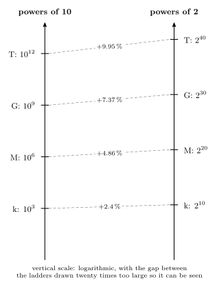
Figure 65: The decimal and binary meanings of each prefix side by side, on a log scale. Each step up the decimal ladder multiplies by 1000 and each step up the binary ladder by 1024, so the binary value pulls a little further ahead at every step: 2.4 per cent at kilo, 4.86 at mega, 7.37 at giga and almost 10 at tera. That is why the ambiguity is a rounding error for a kilobyte but a real difference for a terabyte disk.
Why main memory comes in powers of 2
A memory chip is addressed by address lines, and \(n\) lines can name exactly \(2^n\) cells: one line selects between 2 cells, two lines between 4, three between 8. A memory that used only 1,000,000 of the 1,048,576 addresses its 20 lines can name would waste the rest, so main memory is built in powers of 2 and its size is quoted that way: a “4 GB” module holds \(4 \times 2^{30}\) bytes.
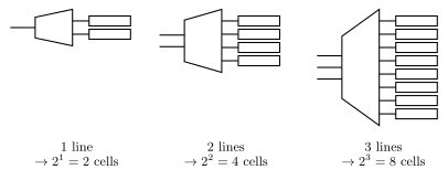
Figure 66: Why memory sizes are powers of 2. With one address line a decoder can select one of 2 cells, with two lines one of 4, and with three lines one of 8: every extra line doubles the number of cells that can be named. So n address lines give exactly 2 to the n cells, and a memory is built to fill that number.
Which convention is used where
| Context | Convention | Example |
|---|---|---|
| Main memory capacity | always powers of 2 | 1 GB \(= 1024 \times 1024 \times 1024\) B \(= 2^{30}\) B |
| Hard disk capacity, as sold | powers of 10 | 1 GB \(= 1000 \times 1000 \times 1000\) B \(= 10^9\) B |
| Operating systems (e.g. Windows) reporting sizes | powers of 2 | a “500 GB” disk shows as about 465.66 GB |
| Data speeds, transfer rates | usually powers of 10 | 1 Gbps (gigabit per second) \(= 10^9\) bits per second |
| Occasionally, a mixture | one of each | the 1.44 MB floppy disk: \(1.44 \times 1000 \times 1024\) bytes |
Disk makers’ powers of 10 make a disk seem bigger. A disk sold as 500 GB holds \(500 \times 10^9\) bytes, and an operating system that divides by \(2^{30}\) reports \(500 \times 10^9 / 2^{30} = 465.66\) “GB”. Nothing is missing; the two numbers use different gigabytes.
Note the case of the b: B is a byte and b is a bit. 1 Gbps is a rate in bits, so it moves \(10^9 / 8 = 125 \times 10^6\) bytes per second at most.
Binary prefixes: KiB, MiB, GiB
To avoid the confusion, standard names were created for the binary meanings:
| Name | Symbol | Value |
|---|---|---|
| kibibyte | KiB | 1024 bytes |
| mebibyte | MiB | 1024 KiB \(= 2^{20}\) bytes |
| gibibyte | GiB | 1024 MiB \(= 2^{30}\) bytes |
With these, kB, MB and GB can keep their SI meanings. Few people use them, though, and these notes use kilo, mega and giga as everyone does, with the meaning depending on the context. When the difference matters, say which one is meant.
Worked: what is a megabyte, and a gigabyte?
How many bytes is 1 MB? How many is 1 GB? How different are the meanings, and how many bytes does a “1.44 MB” floppy disk hold?
1 MB, three ways.
- Conventionally: \(1\text{ MB} = 2^{10}\text{ kB} = 1024\text{ kB} = 2^{20}\text{ B} = \mathbf{1{,}048{,}576}\) B.
- Sometimes, the SI meaning: \(1\text{ MB} = 10^6\text{ B} = \mathbf{1{,}000{,}000}\) B.
- Or in between, with a decimal mega of binary kilobytes: \(1000\text{ kB} = 1000 \times 1024 = \mathbf{1{,}024{,}000}\) B.
1 GB, three ways.
- Conventionally: \(1\text{ GB} = 2^{10}\text{ MB} = 2^{20}\text{ kB} = 2^{30}\text{ B} = \mathbf{1{,}073{,}741{,}824}\) B.
- Sometimes: \(1\text{ GB} = 10^9\text{ B} = \mathbf{1{,}000{,}000{,}000}\) B.
- Or in between: \(1000 \times 2^{20} = \mathbf{1{,}048{,}576{,}000}\) B, a thousand binary megabytes.
How different. The binary gigabyte exceeds the decimal one by \(1{,}073{,}741{,}824 - 1{,}000{,}000{,}000 = 73{,}741{,}824\) bytes, and
\[\frac{73{,}741{,}824}{1{,}000{,}000{,}000} = 0.0737 \approx 7.4\,\%.\]
That 7.4 % is measured against the decimal gigabyte. Measured against the binary one it is \(73{,}741{,}824 / 1{,}073{,}741{,}824 = 6.87\,\%\): the decimal gigabyte is 6.87 % smaller. For the megabyte the gap is \(48{,}576 / 1{,}000{,}000 = 4.86\,\%\). The in-between gigabyte, 1,048,576,000 B, is 4.86 % above \(10^9\) and 2.34 % below \(2^{30}\) (equivalently, \(2^{30}\) is 2.4 % above it).
The floppy disk. Its “1.44 MB” is 1.44 thousand binary kilobytes:
\[1.44 \times 1000 \times 1024 = \mathbf{1{,}474{,}560}\ \textbf{bytes} = 1440\text{ KiB}.\]
That is 1.40625 MiB in binary megabytes and 1.47456 MB in decimal ones. The label is right in neither, which is the point: it mixes a decimal thousand with a binary kilobyte.
Common mistakes
- Calling SRAM “dynamic” because it can be rewritten. Static and dynamic are about how a bit is held, a flip-flop against a leaking capacitor, not about whether it can change. Both are read/write.
- Thinking non-volatile means read-only. Flash and EEPROM are non-volatile and rewritable. ROM is the only one here that can never be rewritten.
- Thinking SRAM keeps its contents at power-off because it does not need refreshing. Static means no refresh while powered. Both SRAM and DRAM are volatile.
- Mixing up flash and EEPROM. Both are electrically erasable; flash erases a block at a time, EEPROM one cell at a time. On the AVR the program goes in flash and individual settings in EEPROM.
- Assuming “MB” has one meaning. Memory sizes are powers of 2, disk sizes and data rates are powers of 10, and some figures mix the two. Say which, or use KiB, MiB, GiB.
- Getting the 7.4 % backwards. \(2^{30}\) is 7.37 % more than \(10^9\), but \(10^9\) is 6.87 % less than \(2^{30}\). The base of a percentage matters.
- Confusing B and b. A 1 Gbps link is about 125 MB/s, not 1 GB/s.
See also
- memory-hierarchy-and-cache — how registers, cache, DRAM and disk are arranged by speed and cost
- magnetic-disks · file-systems — secondary storage and how files are kept on it
- memory-models — the ATmega324A’s address spaces and the three assembler segments
- avr-architecture — flash, SRAM and EEPROM on the chip
- flip-flops-and-latches — the storage element of a static memory cell
- assembly-process —
.cseg,.dsegand.eseg - 2026-10-22-memory-disks-and-files — Lecture 24
Serial Communication
Sending data between devices one bit at a time, and how the receiving end makes sense of what arrives: serial against parallel, synchronous against asynchronous, the UART frame, parity, how a receiver samples the line, and baud rate. Then the synchronous serial buses, where one master clocks data to and from several slaves: SPI and I²C, compared with the UART, and bit bashing for when there is no hardware for a standard. The AVR’s hardware is in avr-usart and avr-spi. First met in 2026-09-24-serial-io and 2026-10-05-more-io.
Serial and parallel
| Parallel | Serial | |
|---|---|---|
| Wires carrying data | one per bit | one |
| How a byte travels | all 8 bits at once | 8 bits one after another |
| Cost | many pins and wires | time: a byte takes 8 bit times |
Inside a chip, data moves in parallel: a port is eight pins, a register is eight flip-flops. Between devices, pins and wires are what is scarce, so nearly every link is serial. The conversion at each end is the job of a shift register (shift-registers): load a byte in parallel and shift it out one bit at a time to send, shift bits in and read the byte out in parallel to receive.
By convention the sending end of a link is Tx and the receiving end is Rx. A device that does both has one of each, and two such devices are joined crossed over: each one’s Tx goes to the other’s Rx.
Synchronous and asynchronous
A receiver has to know when to look at the data wire, as well as what is on it. There are two ways to tell it.
Synchronous: one end sends a clock on a second wire. The receiver reads the data wire on each clock edge. Nothing has to be agreed in advance about speed, beyond the fastest the receiver can follow. SPI, the Serial Peripheral Interface, and I²C both work this way (below).
Asynchronous: there is no clock wire. Each end has its own clock, the two agree on the speed beforehand, and the receiver recovers the exact timing from the data stream itself. That only works if the stream is guaranteed to contain edges to time against, so the data is encoded:
| Encoding | How it guarantees edges | Used by |
|---|---|---|
| start and stop bits | every character begins with a fall from 1 to 0 | UART |
| 4B/5B, 8B/10B | every 4 or 8 bits are replaced by a 5- or 10-bit code that never has a long run | fast network links |
| bit stuffing | an opposite bit is inserted after a run of identical bits | USB at low and full speed |
A UART is a Universal Asynchronous Receiver and Transmitter. A USART can also work synchronously. The pictures of all four cases are in 2026-09-24-serial-io.
The UART frame
A UART sends data in frames. Between frames the line rests at 1, the idle level. A frame is:
| Order | Field | How many | Value |
|---|---|---|---|
| 1 | start bit | 1 | always 0 |
| 2 | data bits | 5 to 9 | the data, least significant bit first |
| 3 | parity bit | 0 or 1 | chosen to make the count of 1s even or odd |
| 4 | stop bits | 1 or 2 | always 1 |
Why each part is there:
- The start bit is 0 because the idle line is 1. The fall from 1 to 0 is the one event the receiver can be sure of, and everything else is timed from it.
- The stop bit is 1 so that the line is back at the idle level when the frame ends. Whatever the last data bit was, the next start bit is then a fall again.
- The data bits go least significant first. A receiver that assumes the opposite reads every byte bit-reversed.
The format is usually written as three items: data bits, parity (N for none, E for even, O for odd), stop bits. 8N1 is 8 data bits, no parity, 1 stop bit, and is by far the commonest.
Worked: the letter s
A character is sent as its ASCII code (c-language-basics). The letter s is 115, 0x73, 0111 0011. In 8N1 the line carries, in time order:
| start | b0 | b1 | b2 | b3 | b4 | b5 | b6 | b7 | stop |
|---|---|---|---|---|---|---|---|---|---|
| 0 | 1 | 1 | 0 | 0 | 1 | 1 | 1 | 0 | 1 |
Read left to right, the data bits are 1100 1110, the byte written backwards.
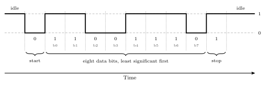
Figure 67: The letter s, 0x73, on the wire as an 8N1 frame. Time runs left to right and each cell is one bit time. The line idles at 1, falls for the start bit, carries the eight data bits least significant first, and returns to 1 for the stop bit. Written most significant bit first the byte is 0111 0011; the wire carries it in the opposite order.
Parity
The parity bit lets the receiver detect that a frame was damaged. The two ends agree on the kind:
- Even parity: the number of 1s in the data bits and the parity bit together is even.
- Odd parity: that number is odd.
To send: count the 1s in the data. Choose the parity bit that makes the total the agreed kind.
To check: count the 1s in the data and the parity bit as received. If the total is the wrong kind, there was an error.
| Data | 1s in the data | Even parity bit | Odd parity bit |
|---|---|---|---|
0xA7 = 1010 0111 |
5 | 1 | 0 |
0xA9 = 1010 1001 |
4 | 0 | 1 |
0x73 = 0111 0011 |
5 | 1 | 0 |
0x00 = 0000 0000 |
0 | 0 | 1 |
The even parity bit is the XOR of the data bits (logic-gates): XOR is 1 exactly when an odd number of its inputs are 1, which is exactly when a 1 is needed to make the total even. The odd parity bit is its complement.
Worked check. 0xA9 arrives with parity bit 1 on an even-parity link. The data has four 1s, and the parity bit makes five. Five is odd, so the frame is in error.
What parity cannot do:
- It cannot say which bit is wrong, so it cannot correct anything. The frame has to be discarded or sent again.
- It misses any even number of flipped bits. Two flips cancel and the count comes out right.
Detecting and correcting needs several check bits arranged so that the pattern of failed checks points at the wrong bit. That is a Hamming code, and it is not part of a UART frame.
Sampling: finding the bits without a clock
The receiver knows the bit time from the agreed baud rate. What it does not know is when a frame will start. It finds out by watching:
- It samples the line many times per bit: 16 on the AVR.
- While the line is idle, every sample is 1. A sample of 0 means a start bit may have begun, and the receiver starts counting samples from there.
- It reads the three samples at the centre of each bit time and takes the majority. For the first bit time the answer must be 0, or the fall was only noise and the receiver goes back to waiting.
- It carries on, one bit time after another, for the data bits, the parity bit if there is one, and the stop bit.
- The stop bit must read 1. If it reads 0 the frame is wrong: a framing error, usually a sign that the two ends disagree about the baud rate or the format.
The picture is in 2026-09-24-serial-io.
Why the clocks need not match exactly. Suppose the receiver’s clock is slightly slow. Each sampling point is then a little later within its bit than the one before, and by the last bit of the frame the lateness has added up. As long as the total stays under half a bit time, every sample still lands inside the right bit. A 10-symbol frame gives the error about ten bit times to build up, so the two clocks have to agree to within a few percent. At the next start bit the count starts again from the new falling edge and the accumulated error is gone. That re-timing on every frame is what the start bit is for.
Baud rate and bit rate
Baud rate = symbols per second. Bit rate = useful data bits per second.
On a UART line a symbol is one bit time, and start, parity and stop bits are symbols that carry no data. So the bit rate is always lower than the baud rate, by the fraction of the frame that is data.
| Format | Symbols per frame | Data bits | Data fraction | At 9600 baud |
|---|---|---|---|---|
| 8N1 | 10 | 8 | 80 % | 7680 bit/s, 960 bytes/s |
| 8E1 or 8O1 | 11 | 8 | 73 % | 6982 bit/s, 873 bytes/s |
| 8N2 | 11 | 8 | 73 % | 6982 bit/s, 873 bytes/s |
| 7E1 | 10 | 7 | 70 % | 6720 bit/s, 960 characters/s |
The method: frames per second is the baud rate divided by the symbols per frame, and bits per second is that times the data bits per frame. For 8N1 at 9600 baud, \(9600 / 10 = 960\) frames per second and \(960 \times 8 = 7680\) bits per second.
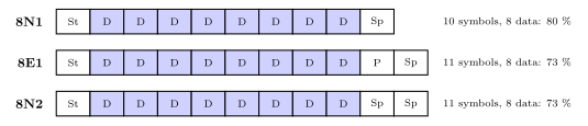
Figure 68: Three frame formats, one cell per symbol. Shaded cells carry data and white cells are framing. Every format here carries eight data bits, so adding a parity bit or a second stop bit makes the frame eleven symbols long instead of ten, and at the same baud rate fewer frames fit into a second.
The standard baud rates are 2400, 4800, 9600, 14400, 19200, 28800, 38400, 57600 and 115200.
Both ends must agree
Four settings define a UART link, and none of them is sent over it:
- the baud rate;
- the number of data bits;
- the parity: none, even or odd;
- the number of stop bits.
A terminal program on a PC asks for all four, plus which serial port to use. If the two ends differ, the receiver still samples the line and still produces bytes. They are just the wrong bytes, sometimes with framing or parity errors flagged and sometimes not. Garbled characters on a terminal almost always mean a mismatch here, most often the baud rate.
RS232
A serial standard more than 40 years old and still in use, typically on a 9-pin D-sub connector. Its frames are UART frames. Its voltages are not the microcontroller’s:
| Microcontroller pin | RS232 line | |
|---|---|---|
| logical 1 | 5 V | negative, −3 V to −15 V |
| logical 0 | 0 V | positive, +3 V to +15 V |
So RS232 is inverted and uses larger voltages of both signs. A level-converter chip such as the MAX-232 goes between an AVR pin and an RS232 line. Connecting the two directly does not work and can damage the pin.
RS232 is full duplex: there is a separate wire for each direction, so both ends can transmit at once. The standard defines many signals, and the smallest useful set is three: TxD, RxD and ground. Ground is needed because a voltage only has meaning against a reference both ends share.
Buses: masters and slaves
A UART joins exactly two devices. A bus is a set of wires shared by several, and that raises the question of who decides when a transfer happens.
- The master initiates and controls the transfer of data: it decides when a transfer starts, which device it is with and which way the data goes, and on a synchronous bus it drives the clock.
- A slave waits for requests and responds to the master. It never starts a transfer.
Some devices can be both, at different times. The AVR’s SPI and TWI ports can each be set up as a master or as a slave, and on an I²C bus more than one device may take a turn at being master. Memory can never be a bus master: all a memory can do is answer a read or a write of an address that something else has chosen. On a processor’s memory bus the CPU is the master.
Synchronous serial buses
Both buses here send a clock from the master alongside the data, so neither needs start and stop bits or an agreed baud rate. They differ in how the master picks which slave it is talking to.
SPI
The Serial Peripheral Interface has four signals: the clock SCK, a data wire each way, MOSI (master out, slave in) and MISO (master in, slave out), and an active-low select \(\overline{\text{SS}}\) for each slave. The master and the slave each hold an 8-bit shift register, and MOSI and MISO join them into a ring, so on every clock pulse one bit goes each way. Eight pulses swap the two bytes: every transfer is an exchange. Several slaves either get a select line each, or are daisy-chained on one select with the data passing through each in turn. All of this, with the AVR’s SPI port, is in avr-spi.
I²C and TWI
I²C, the Inter-Integrated Circuit bus, was created by Philips Semiconductor, now NXP. TWI, the Two-wire Interface, is Atmel’s name for it. There are two wires, and every device connects to both:
- SDA, serial data, which carries data in either direction, one way at a time;
- SCL, serial clock, driven by the master.
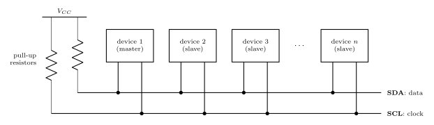
Figure 69: An I²C bus. Every device connects to the same two wires: SDA carries the data, in either direction, and SCL carries the clock from the master. No device ever drives a line high. Each can only pull a line low or let go of it, and the two pull-up resistors hold a line at 1 while nobody is pulling, so two devices can never fight over a line. Because every device hears every transfer, the master begins each one with the address of the slave it is for. A dot is a connection; where a lead crosses SDA without a dot there is no connection.
Why the pull-ups. Every output on the bus is open drain: it can connect its line to ground or leave it alone, and never connects it to \(V_{CC}\). A line is 1 when nobody is pulling it down and 0 when anybody is. Any number of devices can share a wire that way without two outputs ever fighting.
Addresses instead of select lines. Every device sees every transfer, so the master starts each one by sending the address of the slave it wants, and only that slave answers. Adding a device adds no wires.
On the ATmega324A the TWI uses PC0 as SCL and PC1 as SDA, and the datasheet describes it on pages 211 to 239 (2026-10-05-more-io).
UART, SPI and I²C compared
| UART | SPI | I²C / TWI | |
|---|---|---|---|
| Clock | none: both ends agree a baud rate | SCK, from the master | SCL, from the master |
| Data wires | TxD and RxD, one each way | MOSI and MISO, one each way | SDA, shared by both directions |
| Both directions at once? | yes | yes: every transfer is an exchange | no |
| Devices | two | one master, many slaves | many, some able to be master |
| Choosing a slave | no need: only two ends | a select line per slave, or a daisy chain | an address sent on the bus |
| Wires, besides ground | 2 | 3, plus a select per slave | 2 |
| On the ATmega324A | USART0 (PD0, PD1), USART1 (PD2, PD3) | one SPI port, PB4 to PB7 | one TWI port, PC0 and PC1 |
Bit bashing
Sometimes a microcontroller has no hardware support for a bus standard, or not enough interfaces of it. The standard can still be used by simulating it on general purpose port pins: the program sets and clears the output pins and reads the input pins itself, in exactly the order the standard lays down. That is bit bashing, also called bit banging.
Figure 70: Who does the work. Above, with an SPI port: the program writes one byte to the data register and the port’s own clock generator and shift register produce all eight clock pulses and move all sixteen bits, while the CPU is free. Below, bit bashing the same transfer on three ordinary pins of port D: the CPU runs a loop that puts each bit on the MOSI pin, raises and lowers the SCK pin and reads the MISO pin, eight times over, through the port’s PORTD and PIND registers. The slave cannot tell the difference. The CPU is busy for the whole transfer, and the clock can go no faster than the loop.
Worked: an SPI master in software
Three spare pins of port D, plus one for the select, can be an SPI master in mode 0, most significant bit first, with nothing but the set, clear and test idioms of bit-masking:
#define BB_SS    4                 /* port D pins used for the software SPI */
#define BB_SCK   5
#define BB_MOSI  6
#define BB_MISO  7

void bb_init(void) {
    DDRD  |= (1<<BB_SS) | (1<<BB_SCK) | (1<<BB_MOSI);   /* outputs; MISO stays an input */
    PORTD |= (1<<BB_SS);                                /* nothing selected             */
    PORTD &= ~(1<<BB_SCK);                              /* the clock rests low          */
}

uint8_t bb_exchange(uint8_t out) {
    uint8_t in = 0;
    uint8_t i;

    for (i = 0; i < 8; i++) {
        if (out & 0x80) {                    /* put the top bit on MOSI           */
            PORTD |= (1<<BB_MOSI);
        } else {
            PORTD &= ~(1<<BB_MOSI);
        }
        out <<= 1;
        PORTD |= (1<<BB_SCK);                /* rising edge: both ends read       */
        in = (in << 1) | ((PIND >> BB_MISO) & 1);
        PORTD &= ~(1<<BB_SCK);               /* falling edge: the slave moves on  */
    }
    return in;
}
Used like the hardware version: pull BB_SS low, call bb_exchange once per byte, raise BB_SS. Reading MISO straight after raising SCK is safe, because the slave put that bit out on the previous falling edge, or when it was selected, and it stays put until the next falling edge.
What it costs.
- The CPU does everything. Each bit is several instructions, so the clock runs far slower than the 4 MHz the SPI port can make, and the program does nothing else meanwhile.
- Synchronous standards bash easily. The master makes the clock, so if the loop is held up between two edges, by an interrupt for instance, the transfer simply pauses. The slave waits for the next edge however long it takes.
- Asynchronous standards are harder. A bit-bashed UART has no clock to wait for, so every bit time has to be produced exactly, and an interrupt landing in the middle of a frame can wreck it.
Common mistakes
- Tx to Tx. The link is crossed: one end’s transmit pin goes to the other’s receive pin.
- Treating baud rate as bit rate. 9600 baud in 8N1 moves 7680 data bits a second, not 9600.
- Reading the bits most significant first. A UART sends bit 0 first.
- Leaving the parity bit out of the count. The rule is about the data bits and the parity bit together.
- Expecting parity to fix or locate an error, or to catch every error.
- Drawing the idle line at 0. Idle is 1, the start bit is 0, the stop bit is 1.
- Forgetting ground between two boards.
- Crossing SPI’s data wires. MOSI goes to MOSI and MISO to MISO: the names already say which end drives.
- Leaving out the pull-ups on an I²C bus. Nothing ever drives the lines high, so without them they never return to 1.
- Thinking memory could start a transfer. Memory is always a slave.
See also
- avr-usart — the ATmega324A’s USART: registers, baud-rate values, code and interrupts
- avr-spi — the ATmega324A’s SPI port: the exchange, timing, several slaves, registers, clock rate, code
- bit-masking — the set, clear and test idioms the bit-bashing code is made of
- shift-registers — parallel in, serial out, and the reverse
- logic-gates — XOR, which computes a parity bit
- timing-diagrams — how the waveforms here are drawn and read
- magnetic-disks — a disk sector, framed like a UART frame: preamble, data, ECC, gap
- io-board — the USB-serial device that joins the breadboard to a PC
- 2026-09-24-serial-io — Lecture 18 · 2026-10-05-more-io — Lecture 19