MATH1061 — Full Course Notes
Week 1
Lecture 1 — Welcome & Warm-up Problems
Two halves: administration — staff, expectations, support, assessment, the topic list and the schedule — and five warm-up problems that preview the rest of the semester. Everything administrative is in math1061. The few course rules that matter most are repeated here, followed by the problems.
Objectives for the hour
- Introduce the lecturing staff.
- Review course expectations, the course profile and the course website.
- Support mechanisms.
- Explain the assessment structure.
- Topics overview.
The load-bearing bits of the course rules:
- Lectures are Mon 10am, Tue 2pm, Thu 1pm — see the table in math1061.
- General enquiries go to a course address, not a personal one:
math1061@uq.edu.auandmath7861@uq.edu.au. - The pre-class hour is two things: watch videos and answer multiple-choice questions. Both, not just the videos.
- Among the activities: the Active Class, and Complete Assessed Exercises.
- In the assessment: best 8 of 12, and the hurdles on the final exam.
Warm-up problems
Let \(p\), \(q\) and \(r\) be consecutive positive integers with \(p < q < r\), and let \[a = p + r, \qquad b = pr, \qquad c = r - p.\] Determine which of \(a\), \(b\), \(c\) must be even.
Four non-zero real numbers \(a, b, c, d\) are given, where \(b + d \neq 0\). If \(\dfrac{a}{b} + \dfrac{c}{d} = \dfrac{a+c}{b+d}\), show that \(ac < 0\).
True or False: In every group of five people, there are two people who have the same number of friends within the group.
The Tower of Hanoi: Given a tower of 8 discs in decreasing size on one of three pegs, transfer the entire tower to one of the other pegs according to the following rules: (a) Move only one disc at a time. (b) Never move a larger disc onto a smaller disc. Is there a solution? If there is, what is the fewest number of moves needed to complete the transfer?
The Königsberg Bridge Problem: Does there exist a route through the city that crosses each bridge exactly once and takes you back to the starting place? (No turning around on bridges.)
The short answers to the last three: 3 — True, 4 — 255, 5 — No. Problems 1 and 2 are worked in full below.
Solution 1 — parity of \(p+r\), \(pr\) and \(r-p\)
Start with examples, not algebra: \(1,2,3\), then \(5,6,7\), then \(2,3,4\). In each triple look at \(p\) and \(r\), the first and last. What matters is their parity (even/odd): \(p\) and \(r\) are always two apart, so they are always the same kind of number.
Written out: \(p, q, r\) are consecutive, so \[q = p + 1 \qquad\text{and}\qquad r = p + 2.\]
\(a = p + r\) is always even. Since \(r = p+2\), the numbers \(p\) and \(r\) are both even or both odd, and \(\text{even} + \text{even} = \text{even}\) and \(\text{odd} + \text{odd} = \text{even}\). Either way \(a\) is even.
\(b = pr\) is either even or odd, and that is the whole answer. If \(p\) and \(r\) are even then \(pr\) is even; if both are odd then \(pr\) is odd. Nothing forces one case over the other, so \(b\) need not be even.
\(c = r - p\) is always even, and more than that, it is always exactly \(2\): \[c = r - p = (p+2) - p = 2.\]
So \(a\) and \(c\) must be even; \(b\) need not be.
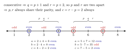
Figure 1: Why two of the three expressions are forced. Consecutive integers alternate parity, so p and r — two apart — always match, which makes p+r even and pinches r−p down to the constant 2; only the product pr is free to go either way. The two windows are the triples 2,3,4 and 5,6,7, with p and r ringed and a, b, c worked out beneath each. Blue marks even and red odd throughout.
Nothing in this solution is more than the definition of “consecutive” plus the two parity facts. That is the shape every direct proof in proof-techniques takes from Lecture 7 onwards. For \(b\), “either even or odd” is a complete answer to “which must be even”, because a single pair of examples on opposite sides settles it.
Solution 2 — showing \(ac < 0\)
The proof is one algebraic chain, ending in an argument about signs:
Suppose \(\dfrac{a}{b} + \dfrac{c}{d} = \dfrac{a+c}{b+d}\).
Put the left side over a common denominator: \[\frac{ad}{bd} + \frac{bc}{bd} = \frac{a+c}{b+d}\]
Multiply both sides by \(bd(b+d)\) — legitimate because \(b, d \neq 0\) and \(b + d \neq 0\), which is exactly why the question hands you those conditions. The \(bd\) cancels on the left and the \(b+d\) on the right: \[bd\,(b+d)\left(\frac{ad+bc}{bd}\right) = \left(\frac{a+c}{b+d}\right)(b+d)\,bd\] \[(ad+bc)(b+d) = (a+c)\,bd\]
Expand the left side (FOIL): \[abd + ad^2 + b^2c + bcd = abd + bcd\]
The \(abd\) and \(bcd\) terms cancel from both sides, leaving \[ad^2 + b^2c = 0, \qquad\text{i.e.}\qquad ad^2 = -b^2 c.\]
Divide both sides by \(ab^2\) (allowed: \(a \neq 0\) and \(b \neq 0\)): \[\frac{d^2}{b^2} = -\frac{c}{a}\]
The left side is a square over a square with \(d \neq 0\), so it is positive; therefore \(-\frac{c}{a}\) is positive, so \(\frac{c}{a}\) is negative. A negative quotient means exactly one of \(a\) and \(c\) is negative, so their product is negative. \(\therefore\; ac < 0\).
Two habits here that the rest of the course keeps asking for. First, every non-zero hypothesis gets used at the moment it licenses a division — the three conditions \(b \neq 0\), \(d \neq 0\), \(b + d \neq 0\) are not decoration. Second, the final step reasons about sign, not about values: \(\frac{c}{a} < 0\) says one of the two is negative without saying which, and that is already enough for \(ac < 0\).
The symbol \(\therefore\) reads “Therefore”. It prefixes the conclusion of an argument all semester (see math1061-diagram-notation).
Solutions 3, 4 and 5
Each of these answers is the punchline of a topic later in the semester.
3. True — and it is the pigeonhole principle
True. Each of the five people has a friend count somewhere in \(\{0, 1, 2, 3, 4\}\) — five people, five possible values, so counting alone is not enough. The extra fact is that \(0\) and \(4\) cannot both occur: if someone is friends with all four others, then nobody has zero friends; and if someone has zero friends, nobody can be friends with all four. So the counts actually available are only four values, and five people distributed over four values must repeat one. That is the pigeonhole principle, which arrives in Lecture 33 — see pigeonhole-principle, where the same argument is made for the degrees of a graph, and practice-problems.
(This assumes friendship is mutual, which is what “friends within the group” is taken to mean.)
4. 255 moves
255. The reasoning comes in Lecture 16 and is worked in full at solving-recurrence-relations: letting \(m_n\) be the minimum number of moves for \(n\) discs, moving the largest disc forces the other \(n-1\) onto the spare peg and back again, giving \[m_1 = 1, \qquad m_k = 2m_{k-1} + 1 \;\text{ for } k \geq 2,\] whose explicit formula is \(m_n = 2^n - 1\). For eight discs, \(2^8 - 1 = 255\). The answer to “is there a solution?” is yes, and constructively so — the recursion is the algorithm.
5. No
No. The modelling step is to redraw the map of Königsberg, a river crossed by seven bridges, as a graph. Graph theory is introduced at Lecture 33; the graph theory lectures are L33–L36. Graphs, loops, multiple edges and degree are defined in [graphs].
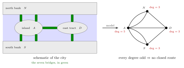
Figure 2: The modelling step. Each land mass becomes a vertex and each bridge an edge, so the seven bridges become seven edges on four vertices — and the question ‘can I walk every bridge once and get back?’ becomes a question about degrees. Every vertex here has odd degree, and a closed route must enter and leave each land mass in pairs, so no such route exists. The left panel is a schematic of the city, with the land masses named A, N, S and D and the bridges in green; the right panel is the same city as a graph.
The question as asked is for a closed route — one that returns to where it started. Such a route must leave every land mass exactly as often as it enters it, so every bridge at a land mass is used in an entry/exit pair, and every vertex must have even degree. Here all four are odd, so no closed route exists.
Keep the two criteria apart. The standard slogan is about the open case: an open route crossing every bridge once (not required to return) exists only when the number of odd-degree vertices is \(0\) or \(2\). Königsberg has four, so that fails too — but “more than two odd vertices” is not the criterion for the question as asked.
Both criteria are the two halves of one theorem about connected graphs: an Euler circuit exists exactly when every vertex has even degree, and an Euler trail between two different vertices exactly when those two are the only odd ones. The theorem, its proof and how to find such a route are in euler-circuits-and-trails, and Lecture 34 (2026-10-26-walks-trails-and-circuits) applies it.
What each problem previews
| Problem | Previews | Lecture |
|---|---|---|
| 1 — parity of \(p+r\), \(pr\), \(r-p\) | direct proof, definitions of even/odd, number theory | L7 (proof-techniques) |
| 2 — showing \(ac < 0\) | direct proof from an algebraic hypothesis; using every hypothesis | L7 (proof-techniques) |
| 3 — five people, same friend count | the pigeonhole principle | L33 (pigeonhole-principle) |
| 4 — Tower of Hanoi | recursion, recurrence relations, induction | L13–L16 (solving-recurrence-relations) |
| 5 — Königsberg bridges | graph theory, walks and circuits | L33–L34 ([graphs], euler-circuits-and-trails) |
That table is the course outline in miniature — logic and proof first, then number theory, sets, functions and relations, group theory, counting, and graph theory last. Fields and probability belong to the same stretch of the semester; see math1061 for the course profile’s topic list. Some of this overlaps Year 11 and 12 Specialist Mathematics.
See also
- math1061 — staff, assessment weights, support, and the lecture schedule
- math1061-diagram-notation — the course’s own notation and figure conventions
- 2026-07-30-logical-form-and-equivalence — Lecture 2, where the symbolic logic starts properly
- proof-techniques — the four proof methods problems 1 and 2 are a warm-up for
- solving-recurrence-relations — the Tower of Hanoi recurrence worked in full
- euler-circuits-and-trails — the theorem that settles the bridges of Königsberg
- practice-problems — the semester-wide practice problem set, with solutions; it belongs to the individual-study hours, not the class (the logic sections begin at practice-problems)
Lecture 3 — Conditional Statements
Pre-work: Video 003 (Conditional Statements). See conditional-statements for the reference definitions this lecture builds on. Note: Applied Classes start in Week 2, and they include an assessed component.
The proofs of \(\sim\big((\sim p \land q) \lor (\sim p \,\land\sim q)\big) \equiv p\) — one by truth table and two by chains of laws — are at the end of Lecture 2.
Learning goals
- Understand the connectives if…then (\(\to\)) and if and only if (\(\leftrightarrow\)).
- Be familiar with common logical equivalences involving if…then: \[p \to q \;\equiv\; \sim p \lor q \;\equiv\; \sim q \,\to\, \sim p\] Know this — the two rewrites are the whole toolkit for everything below.
- Be able to negate a conditional statement.
- Understand the meaning of necessary and sufficient conditions.
Common questions
- How can \(p \to q\) be true when \(p\) is false? Because that is how it is defined. The bottom two rows of the table are a definition, not a claim about the world.
- Can we use any laws for “\(p\) implies \(q\)”? Replace \(p \to q\) with \(\sim p \lor q\) and then use the laws. The laws of logical equivalence are stated only for \(\sim, \land, \lor\), so this substitution is what gives you access to them.
- For necessary and sufficient conditions, which one signifies IF, and which ONLY IF? “If” is the sufficient half, “only if” is the necessary half.
Conditional (\(\to\))
| \(p\) | \(q\) | \(p \to q\) |
|---|---|---|
| T | T | T |
| T | F | F |
| F | T | T |
| F | F | T |
Exactly one row makes it false: true hypothesis, false conclusion. See the containment figure in conditional-statements: the situations making \(p\) true sit inside the situations making \(q\) true, which is why nothing outside \(p\) can falsify the conditional.
By definition — this is also called the disjunctive form of \(\to\) —
\[p \to q \;\equiv\; \sim p \lor q\]
Contrapositive, converse, inverse
| Name | Form | |
|---|---|---|
| Conditional | \(p \to q\) | logically equivalent to each other |
| Contrapositive | \(\sim q \,\to\, \sim p\) | |
| Converse | \(q \to p\) | logically equivalent to each other |
| Inverse | \(\sim p \,\to\, \sim q\) |
Reminder: \(p \to q \not\equiv q \to p\). The four forms and the only equivalences among them are laid out as a figure in conditional-statements.
English phrasings
\(p \to q\) can be expressed in many ways in English. The following are logically equivalent:
- \(p\) implies \(q\)
- If \(p\) then \(q\)
- \(q\) if \(p\)
- \(p\) is sufficient for \(q\)
- \(p\) only if \(q\)
- \(q\) is necessary for \(p\)
Watch where the letters land: “\(q\) if \(p\)” puts the hypothesis second, and “\(p\) only if \(q\)” puts the hypothesis first. Those two lines are the ones worth memorising, because they are the ones the necessary/sufficient vocabulary is built on.
Biconditional
\[p \leftrightarrow q \;\equiv\; (p \to q) \land (q \to p)\]
Worked: equivalents and negation of a conditional
(a) Which of the following statements have the same meaning as: “If the file is missing, then the program crashes”? (Multiple answers allowed.)
Let \(p\) = “the file is missing” and \(q\) = “the program crashes”, so the statement is \(p \to q\).
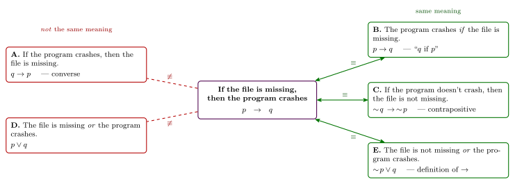
Figure 3: The five options and their verdicts, each translated into symbols: green has the same meaning as the original, red does not. The verdict follows from the symbols alone: B is the same conditional with the ‘if’ clause second, C is its contrapositive, E is its disjunctive form. A is the converse and D is a plain disjunction — neither is equivalent. Translate before judging: A and B are built from the same two clauses in the same order — all that moves is which clause the ‘if’ attaches to, and that alone reverses the conditional.
Answer: B, C and E.
(b) Write the NEGATION of the original statement.
\[\sim(p \to q) \;\equiv\; \sim(\sim p \lor q) \;\equiv\; p \,\land\sim q\]
by the definition of \(\to\), then De Morgan’s law and the double negative law. In English:
The file is missing but the program didn’t crash.
The negation of a conditional is an and, never another conditional.
Worked: the inverse is not the negation
Demonstrate that \(\sim(p \to q) \;\not\equiv\; \sim p \,\to\, \sim q\).
Let \(p\) be true and \(q\) be true. Then \((p \to q)\) is true, so \(\sim(p \to q)\) is false. BUT \(\sim p \,\to\, \sim q\) is true. \(\therefore \; \sim(p \to q) \;\not\equiv\; \sim p \,\to\, \sim q\).
The third line holds because \(\sim p \,\to\, \sim q\) evaluates as \(\mathrm{F} \to \mathrm{F}\), true by the bottom row of the table. This is the shape for demonstrating \(\not\equiv\): name one assignment, evaluate both sides on it, then state the conclusion. No truth table required.
\(\sim p \,\to\, \sim q\) is the inverse — offering it as the negation of \(p \to q\) is the classic error that learning goal 3 is aimed at.
Order of operations (extended)
- \(\sim\)
- \(\land, \lor\) (equal) — use parentheses to specify; if none, work from left to right
- \(\to, \leftrightarrow\) (equal) — use parentheses to specify; if none, work from left to right
So the statement form \(p \,\to\, \sim q \lor r\) means \(p \to \big((\sim q) \lor r\big)\), but parentheses should always be used to avoid confusion.
Note on notation. The biconditional \(\leftrightarrow\) is a connective, used to combine statements (similar to \(+, -, \times, \div\) … with numbers). Logical equivalence \(\equiv\) is used when comparing two statements (similar to \(=\) with numbers). Do not blur the two: \(a \leftrightarrow b\) is itself a statement, \(a \equiv b\) is a claim about two statements.
Worked: an equivalence proved two ways
Let \(p, q\) and \(r\) be statements. Show that \(p \to (q \lor r) \;\equiv\; (p \,\land\sim q) \to r\).
There are two solutions.
Solution 1 — one chain, all the way across:
\[ \begin{aligned} p \to (q \lor r) &\equiv \sim p \lor (q \lor r) && \text{by definition of } \to \\ &\equiv (\sim p \lor q) \lor r && \text{by the associative law} \\ &\equiv (\sim p \,\lor\sim\sim q) \lor r && \text{by the double negative law} \\ &\equiv \sim(p \,\land\sim q) \lor r && \text{by De Morgan's law} \\ &\equiv (p \,\land\sim q) \to r && \text{by definition of } \to \end{aligned} \]
Solution 2 — work both sides down to the same thing:
\[ \begin{aligned} \text{LHS:}\quad p \to (q \lor r) &\equiv \sim p \lor (q \lor r) && \text{definition of } \to \\ &\equiv (\sim p \lor q) \lor r && \text{associative} \\[6pt] \text{RHS:}\quad (p \,\land\sim q) \to r &\equiv \sim(p \,\land\sim q) \lor r && \text{definition of } \to \\ &\equiv (\sim p \lor q) \lor r && \text{De Morgan's and double negative} \end{aligned} \]
Both sides reach \((\sim p \lor q) \lor r\) — the same — so the two forms are equivalent.
Solution 2 avoids having to guess which direction to push a negation — each side is simplified independently until they meet. Both are complete proofs.
Necessary and sufficient conditions
\(p\) is a necessary condition for \(q\) means “if \(\sim p\) then \(\sim q\)”, or equivalently “if \(q\) then \(p\)” (\(q \to p\)), or “\(q\) only if \(p\)”.
\(p\) is a sufficient condition for \(q\) means “if \(p\) then \(q\)”, or equivalently “\(q\) if \(p\)”.
The two phrasings of necessary are contrapositives of each other, which is why they agree.
Worked — necessary but not sufficient. Being a non-negative integer is necessary for a number to be the square of an integer, but it is not sufficient.
- If a number is the square of an integer, then it is non-negative — so \(-9\) cannot be the square of an integer.
- But \(7\) is a non-negative integer and is not the square of an integer, so the condition does not suffice.
Worked — sufficient but not necessary. Being an integer that is divisible by 4 is sufficient for being an even integer, but it is not necessary.
- \(8\) is divisible by 4, so we know that \(8\) is even — no further checking needed.
- But \(10\) is an even integer and is not divisible by 4, so the condition is not required.
Biconditional as necessary and sufficient
The three rows below say the same thing, and each splits at the same seam:
| Whole statement | the necessary half | the sufficient half | ||
|---|---|---|---|---|
| \(a \leftrightarrow b\) | \(\equiv\) | \((a \to b)\) | \(\land\) | \((b \to a)\) |
| \(a\) if and only if \(b\) | \(\equiv\) | \(a\) only if \(b\) | and | \(a\) if \(b\) |
| \(b\) is necessary and sufficient for \(a\) | \(\equiv\) | \(b\) is necessary for \(a\) | and | \(b\) is sufficient for \(a\) |
Read down the third column and you get three names for one half of the biconditional; down the fifth, three names for the other. That answers the earlier question: “only if” marks the necessary half, “if” marks the sufficient half. The same table is a colour-aligned figure in conditional-statements.
Worked: conditions for divisibility by 6
Let \(n\) be a positive integer.
| Asked | Answer | Why | |
|---|---|---|---|
| (a) | A condition necessary but not sufficient for \(n\) to be divisible by 6 | \(n\) is divisible by 3 | Every multiple of 6 is a multiple of 3, so it is necessary; \(n = 3\) is divisible by 3 but not by 6, so it is not sufficient |
| (b) | A condition sufficient but not necessary for \(n\) to be divisible by 6 | \(n = 12\) | \(12\) is divisible by 6, so it suffices; \(n = 6\) is divisible by 6 without being \(12\), so it is not necessary |
| (c) | A necessary and sufficient condition for \(n\) to be divisible by 6 | \(n\) is divisible by both 2 and 3 | Both directions hold, so this is a genuine biconditional |
A sufficient but not necessary condition can be cheap — pinning \(n\) to a single value is sufficient for anything true of that value.
See also
- conditional-statements — the reference definitions, the four forms, and the necessary/sufficient vocabulary
- logical-equivalence-laws — the laws used in the negation and the two-way proof above
- 2026-07-30-logical-form-and-equivalence — Lecture 2 · 2026-08-03-valid-and-invalid-arguments — Lecture 4
- practice-problems — §3 Conditional Statements, with full worked solutions
Lecture 2 — Logical Form and Logical Equivalence
Pre-work: Video 001 (Logical Form), Video 002 (Logical Equivalence). See logical-connectives and logical-equivalence-laws for the reference definitions/tables this lecture builds on.
Logic is the study of reasoning. What the language of symbolic logic is for is worth keeping in view, because the rest of the logic block is in service of it. Symbolic logic will help us to:
- analyse ordinary sentences,
- test arguments for validity,
- construct proofs for complex arguments,
- identify incorrect proofs and common fallacies.
Learning goals
- Appreciate the difficulties in translating between English and mathematics.
- Understand the logical connectives \(\sim\) (not), \(\land\) (and), \(\lor\) (or).
- Construct a truth table for a statement form in standard form.
- Use a truth table to establish logical equivalence of two statement forms.
- Apply logical equivalence laws to establish logical equivalence of two statement forms.
Common questions
- Can we use other symbols for “not”? Yes — common symbols for not include \(\sim\) and \(\neg\). This course writes \(\sim\).
- How do we work out the number of variables and the number of rows in a truth table — for \((p \land q) \land (q \land r)\), are there 2 variables, 3 or 4? Each unique letter is a variable, so here there are 3 variables \(p, q, r\), and the truth table has \(2^3 = 8\) rows. The repeated \(q\) does not count twice.
- Do we need to memorise the laws of logical equivalence? No. The laws are given on the examination formula page (see formula-sheet).
Statements
A statement (or proposition) is a sentence that is either true or false, but not both.
- Statements: “6 is odd.” — a statement, and false. “It is raining.” — also a statement; it could be either true or false, and not knowing the value doesn’t stop it having one.
- Not statements: “\(x\) is odd.” (depends on the unspecified \(x\)), “Is it raining?” (a question), “She is happy.” (not objectively true or false).
We use variables \(p, q, r, \dots\) to represent statements, and the connectives and \(\land\), or \(\lor\), not \(\sim\) to combine them. See logical-connectives.
Worked: translating between English and symbols
Let \(p\) = “it is cold”, \(q\) = “it is snowing”, \(r\) = “it is sunny”.
Into symbolic form:
| English | Symbolic | Note |
|---|---|---|
| It is not cold but it is snowing. | \(\sim p \land q\) | “but” is \(\land\) — the contrast it carries in English is invisible to logic |
| It is neither snowing nor cold, but it is sunny. | \(\sim(q \lor p) \land r \;\equiv\; (\sim q \,\land\sim p) \land r\) | “neither … nor” is the negation of an “or” statement; the second form is the De Morgan rewrite of the first |
Into English:
| Symbolic | English |
|---|---|
| \(\sim q \land p\) | It is not snowing and it is cold. |
| \((p \land q) \lor r\) | It is cold and snowing, or it is sunny. |
The \(\lor\) in the second one is the inclusive or — a day that is cold, snowing and sunny satisfies it.
Are these equivalent statements? (1) “It is not cold but it is snowing.” (2) “It is snowing and it is not cold.”
Yes — by the commutative law. Symbolically \(\sim p \land q \equiv q \,\land\sim p\). The English word order carries an emphasis the logic does not.
Truth tables
A truth table shows the truth value of a statement form for all possible truth values of its statement variables. With \(n\) variables it has \(2^n\) rows. You should know the truth tables for \(\land\), \(\lor\) and \(\sim\) by heart.
Build them in standard form, so that you are sure you have covered all combinations and it is easy for someone to check your work — the fixed row order is drawn out as a figure in logical-connectives.
Inclusive and exclusive or
\(\lor\) means inclusive or: \(p \lor q\) is true when \(p\) is true, or \(q\) is true, or both.
Sometimes English “or” means “one or the other but not both” — exclusive or, written \(\oplus\) (XOR):
\[p \oplus q \;\equiv\; (p \lor q) \land \big(\sim(p \land q)\big)\]
Setting \(p \oplus q\) between \(p \land q\) and \(p \lor q\) makes the two differences visible:
| \(p\) | \(q\) | \(p \land q\) | \(p \oplus q\) | \(p \lor q\) |
|---|---|---|---|---|
| T | T | T | F | T |
| T | F | F | T | T |
| F | T | F | T | T |
| F | F | F | F | F |
\[p \oplus q \;\not\equiv\; p \lor q \qquad\qquad p \oplus q \;\not\equiv\; p \land q\]
Examples from common English usage: “Would you like red or white wine?” is exclusive and “Would you like milk or sugar with your tea?” is inclusive. Only context distinguishes them — which is precisely learning goal 1.
Order of operations
- \(\sim\) first.
- \(\land\) and \(\lor\) equal second — use parentheses to specify; if no parentheses, work from left to right.
Worked. Take the statement form \((p \land q) \lor \sim (r \lor p) \land s\). This means
\[\big((p \land q) \lor (\sim (r \lor p))\big) \land s\]
\(\sim\) takes only \((r \lor p)\); the remaining \(\lor\) and \(\land\) are then equal in precedence, so they resolve left to right.
Worked: constructing a truth table
Construct a truth table for \((p \,\land\sim q) \lor (q \land r)\).
There are two ways to lay this out: give each sub-expression its own column (\(\sim q\), then \(p \,\land\sim q\), then \(q \land r\), then the whole thing), or work all at once, writing each column of values directly beneath the part of the expression it evaluates. The figure below uses the column-by-column layout, because a single column can then be checked in isolation.
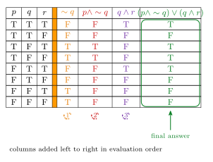
Figure 4: The truth table for (p ∧ ~q) ∨ (q ∧ r), laid out column by column. The evaluation order is numbered ①②③ beneath — ~q first, then p ∧ ~q, then q ∧ r — and the outlined last column is the final answer. Laid out this way, any one column can be checked in isolation.
Logical equivalence
Given two statement forms, you can show that they are logically equivalent (\(\equiv\)) using a truth table or the laws of logical equivalence. To show that two statement forms are not logically equivalent (\(\not\equiv\)), you need to find a set of truth values for the variables for which the two statement forms have opposite truth values.
Worked: a non-equivalence from one row
Show that \(\sim(p \lor q) \;\not\equiv\; \sim p \lor \sim q\).
Take \(p\) false and \(q\) true:
- LHS: \(p \lor q\) is \(\mathrm{F} \lor \mathrm{T} = \mathrm{T}\), so \(\sim(p \lor q)\) is false.
- RHS: \(\sim p \,\lor\sim q\) is \(\mathrm{T} \lor \mathrm{F} = \mathrm{T}\), so it is true.
They differ on this assignment, so they are not logically equivalent. One row is a complete answer — there is no need to fill in the other three.
De Morgan’s Laws
Important logical equivalences for the negations of statements involving “and” and “or”:
\[\sim(p \land q) \equiv \sim p \lor \sim q \qquad\qquad \sim(p \lor q) \equiv \sim p \land \sim q\]
Both halves get negated and the connective flips. The non-equivalence above is what happens when you flip the sign but forget the connective.
Worked: negating an “and” statement
Write down a statement which is logically equivalent to the NEGATION of: “5 is divisible by 2 and 6 is divisible by 2.”
5 is not divisible by 2 or 6 is not divisible by 2.
(The original is \(p \land q\) with \(p\) = “5 is divisible by 2” and \(q\) = “6 is divisible by 2”, so its negation is \(\sim p \,\lor\sim q\). As it happens the negation is true and the original false, but that is not what was asked — the question is about form.)
The laws of logical equivalence
The full table is in logical-equivalence-laws; it is the one on the examination formula page. Two definitions used throughout it:
- a tautology \(\mathbf{t}\) is a statement that is always true;
- a contradiction \(\mathbf{c}\) is a statement that is always false.
Worked: two proofs with the laws
Show that \((p \,\land\sim q) \land (\sim p \lor q) \equiv \mathbf{c}\).
\[ \begin{aligned} (p \,\land\sim q) \land (\sim p \lor q) &\equiv (p \,\land\sim q) \;\land\; \sim(p \,\land\sim q) && \text{by De Morgan's law and the double negative law} \\ &\equiv r \,\land\sim r \quad \text{where } r = (p \,\land\sim q) \\ &\equiv \mathbf{c} && \text{by the negation law} \end{aligned} \]
The move that makes it short is recognising \(\sim p \lor q\) as \(\sim(p \,\land\sim q)\) — a whole compound expression standing in for the single letter the law is written with.
Show that \(\sim p \lor (p \land q) \;\equiv\; \sim p \lor q\).
\[ \begin{aligned} \sim p \lor (p \land q) &\equiv (\sim p \lor p) \land (\sim p \lor q) && \text{by the distributive law} \\ &\equiv \mathbf{t} \land (\sim p \lor q) && \text{by the negation law} \\ &\equiv \sim p \lor q && \text{by the identity law} \end{aligned} \]
Worked: one equivalence, by truth table and by the laws
(a) Use a truth table to show that \(\sim\big((\sim p \land q) \lor (\sim p \,\land\sim q)\big) \equiv p\).
| \(p\) | \(q\) | \(\sim p\) | \(\sim q\) | \(\sim p \land q\) | \(\sim p \,\land\sim q\) | \((\sim p \land q) \lor (\sim p \,\land\sim q)\) | \(\sim\big(\cdots\big)\) |
|---|---|---|---|---|---|---|---|
| T | T | F | F | F | F | F | T |
| T | F | F | T | F | F | F | T |
| F | T | T | F | T | F | T | F |
| F | F | T | T | F | T | T | F |
The first column and the last column are identical, so \(\sim\big((\sim p \land q) \lor (\sim p \,\land\sim q)\big) \equiv p\). Marking the two columns that have to match — with a \(\ast\) beneath each — and then stating the verdict in words is how to finish a truth-table equivalence proof. The table alone does not say what it has shown.
(b) Use the laws of logical equivalence to show the same.
There are two complete chains, one six steps and one four. Both are drawn side by side as a figure in logical-equivalence-laws; the short one comes from noticing that \(\sim p\) is a common factor of the two disjuncts and pulling it out with the distributive law before doing anything else.
See also
- logical-connectives · logical-equivalence-laws — the reference definitions and the full table of equivalence laws
- formula-sheet — why the laws don’t need memorising
- 2026-07-30-conditional-statements — Lecture 3
- practice-problems — §1 Logical Form, with full worked solutions
- practice-problems — §2 Logical Equivalence, with full worked solutions
Week 2
Lecture 4 — Valid and Invalid Arguments
Pre-work: Video 004 (Valid & Invalid Arguments), Video 005 (Methods for Determining Validity). See valid-argument-forms for the reference definitions/table this lecture builds on.
Learning goals
- Understand the difference between a valid argument and an invalid argument.
- Use a truth table to determine the validity of an argument.
- Use rules of inference to demonstrate the validity of an argument.
- Look for truth values that demonstrate an argument is invalid.
Recall
\[p \to q \;\equiv\; \sim p \lor q \;\equiv\; \sim q \to \sim p\]
\(\sim p \lor q\) is the definition of \(\to\), and \(\sim q \to \sim p\) is the contrapositive. Both are used as justifications in Argument 1(c) below — line 3 is the contrapositive, line 6 the definition of \(\to\) — so it is worth having them to hand before starting.
Valid vs invalid arguments
An argument is a sequence of statements — premises and a conclusion. An argument is valid if the conjunction of the premises implies the conclusion: whenever all of the premises are true, the conclusion is also true. Stated as one formula, the argument is valid exactly when
\[(\text{Premise}_1 \land \text{Premise}_2 \land \cdots \land \text{Last Premise}) \to \text{Conclusion}\]
is a tautology.
The first example is the pink shirt argument — “if today is Monday, then I am wearing a pink shirt; today is Monday; therefore I am wearing a pink shirt” — which is valid even though its first premise is false and its conclusion is false. Its form is Modus Ponens. It is worked both ways (row check and tautology check) in determining-argument-validity.
See valid-argument-forms for the formal definition and the standard forms (Modus Ponens, Modus Tollens, etc.).
Questions about validity
How can you have a valid argument with a false conclusion? The pink shirt argument is one. Validity is a property of the form, not of the facts. It says the conclusion follows if the premises hold; it never claims they do.
Why is an argument valid if it has a false premise? The premises sit in the antecedent of \((\text{Premise}_1 \land \cdots) \to \text{Conclusion}\). A false premise makes that conjunction false, and a conditional with a false antecedent is true (the two \(\text{F}\)-antecedent rows of the \(p \to q\) table). So a row containing a false premise is true whatever the conclusion does, and can never break the tautology. It does not follow that an argument with a false premise is automatically valid: the rows where every premise is true still have to be checked.
Do we have to memorise the rules of inference? No. The forms table is on the MATH1061/MATH7861 Examination Formula Page, so the list is in front of you in the exam and the work left to do is recognising which form an argument matches and naming it in a justification.
Three arguments, three methods
Three arguments, worked by three different methods. Full solutions for all of them are in determining-argument-validity.
Argument 1: Let \(w\) = “wages are raised”, \(b\) = “buying increases”, \(d\) = “there is a depression”.
If wages are raised, buying increases. If there is a depression, buying does not increase. Therefore there is not a depression or wages are not raised.
- (a) Write this argument in symbolic form. → \(w \to b\), \(\;d \to \sim b\), \(\;\therefore \sim d \lor \sim w\).
- (b) Use a truth table to determine whether the argument is valid. → Valid: build the eight-row table with \(\sim w\), \(\sim b\), \(\sim d\) as helper columns, find the four rows where both premises are T (rows 2, 6, 7, 8), and check the conclusion is T in each.
- (c) Use the laws of logical equivalence and rules of inference to show the argument is valid. → Valid: contrapose premise 2 into \(b \to \sim d\), chain with premise 1 by Transitivity, then unpack \(w \to \sim d\) into the required disjunction.
Argument 2 (Q1 from the Methods video pre-class questions):
\[ \begin{aligned} &1. \quad p \to q \\ &2. \quad p \lor r \\ &3. \quad p \;\lor \sim r \\ &\therefore \quad q \end{aligned} \]
- (a) Use the laws of logical equivalence and rules of inference to show this argument is valid. → Valid: conjoin the two disjunctive premises, distribute, and \(p\) falls out; Modus Ponens finishes it.
- (b) Alternatively, try to find truth values that make all the premises true but the conclusion false — if none exist, the argument is valid. → None exist: the search forces \(r\) to be both true and false.
Argument 3 (Q2 from the Methods video pre-class questions):
\[ \begin{aligned} &1. \quad p \to q \\ &2. \quad q \to r \\ &3. \quad \sim p \;\lor \sim q \\ &\therefore \quad r \end{aligned} \]
Try to find truth values that make all the premises true but the conclusion false. → They exist: \(p\), \(q\), \(r\) all false makes every premise true and the conclusion false, so this argument is invalid.
Extra practice: revisit Argument 1 — run the same invalidity search on it. The conclusion being false forces \(d\) and \(w\) both true, premise 1 then forces \(b\) true, and premise 2 is now false. Contradiction, so Argument 1 is valid a third time.
Driving a rules-of-inference proof
Each of the two rules-of-inference proofs is steered towards one form: Transitivity for Argument 1(c), Modus Ponens for Argument 2(a). They land in different places — Transitivity is the pivot of Argument 1(c), at line 5 of 7, while Modus Ponens is the last line of Argument 2(a). The question to ask of each argument is how to reach that form: “how can I use transitivity?” for Argument 1(c), and “how can I get to show \(p\)?” for Argument 2(a).
The habit is to pick the valid argument form you want to reach, then work out what has to be manufactured from the premises to fire it. It is the transferable part, and both proofs are consistent with it.
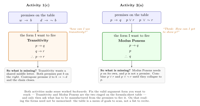
Figure 5: The two rules-of-inference proofs, Argument 1(c) and Argument 2(a), arranged around the form each one is steered towards: Transitivity (orange border) and Modus Ponens (green border). Each panel goes from the premises to the form to reach, and then to what is still missing to fire it. Worked backwards like this, the forms table is a menu of goals to scan, not a list to recite.
Every derived line needs a written justification. Naming the law or form applied, and the lines it came from (“from ② by contrapositive”; “from ① & ④ by transitivity”), is part of the answer, not a courtesy.
Which method to reach for
| truth table | rules of inference | invalidity search | |
|---|---|---|---|
| Used here on | the pink shirt example, Argument 1 | Arguments 1, 2 | Arguments 1, 2, 3 |
| Can prove valid | yes | yes | yes |
| Can prove invalid | yes | no | yes |
| Effort with \(n\) variables | \(2^n\) rows | varies; may stall | usually a handful of forced values |
| Gives you the counterexample | you have to spot the row | never | yes, directly |
The invalidity search is the only method used on all three arguments, and Argument 3 — the one invalid argument of the three — can only be settled by it or by a full truth table. A stalled rules-of-inference attempt proves nothing at all.
See also
- valid-argument-forms — the named argument forms (Modus Ponens, Modus Tollens, Elimination, Generalization, Specialization, as the formula page spells them)
- determining-argument-validity — the truth-table, rules-of-inference and invalidity methods worked through on all three arguments
- logical-equivalence-laws — the laws the inference proofs lean on
- 2026-07-30-conditional-statements — Lecture 3 · 2026-08-06-quantified-statements — Lecture 5
- practice-problems — §4 Valid and Invalid Arguments, with full worked solutions
- practice-problems — §5 Methods for Determining Validity, with full worked solutions
Lecture 6 — Multiple Quantifiers, Negations of Quantified Statements
Pre-work: Video 007 (Negation of Quantified Statements), Video 008 (Statements with Multiple Quantifiers). See quantified-statements for the reference rules and tables this lecture builds on.
Learning goals
- Know how to negate quantified statements.
- Understand and analyse statements with multiple quantifiers.
- Know how to negate statements with multiple quantifiers.
Common questions
If we establish that the negation of a statement is true, does that mean the original statement is false? Yes.
Negations of quantified statements — why does “exists” change to “for all” and vice versa? “Not every \(x\) has property \(P\)” is exactly “some \(x\) fails \(P\)”, and “no \(x\) has property \(P\)” is exactly “every \(x\) fails \(P\)”. The rules themselves are in quantified-statements.
Is there a short-hand way to write “such that”? Where do we place it? s.t., immediately after the variable and its domain: \(\exists x \in D\) s.t. \(P(x)\).
How can we tell whether a statement with multiple quantifiers is true or false? Sometimes it helps to consider both the original statement and its negation. Remember:
- \(\forall x \in D \dots\) can be shown false with one example.
- \(\exists x \in D \dots\) can be shown true with one example.
Worked: a negation is not the “opposite-sounding” statement
The truth of each statement for each set \(S\):
| \(S\) | \(\forall x \in S, x\) is odd | \(\forall x \in S, x\) is not odd | \(\exists x \in S\) s.t. \(x\) is not odd |
|---|---|---|---|
| \(\{1,3,5,7\}\) | T | F | F |
| \(\{1,2,3,4\}\) | F | F | T |
| \(\{2,4,6,8\}\) | F | T | T |
The first and third columns are negations of one another — they disagree in every row. The middle column is not the negation: for \(S = \{1,2,3,4\}\) it and the original are both false, so they can’t be negations.
Q2 from the Video 7 pre-class questions
Which of the following is a negation of \(\forall x \in \mathbb{Z}\), if \(x^2 > 3\) then \(x > 3\)?
- \(\exists x \in \mathbb{Z}\) such that \(x^2 \leq 3\) or \(x > 3\).
- \(\forall x \in \mathbb{Z}\), if \(x > 3\) then \(x^2 > 3\).
- \(\exists x \in \mathbb{Z}\) such that if \(x^2 > 3\) then \(x > 3\). d. \(\exists x \in \mathbb{Z}\) such that \(x^2 > 3\) and \(x \leq 3\).
- \(\exists x \in \mathbb{Z}\) such that \(x^2 \geq 3\) and \(x \geq 3\).
Answer: d. The trap is that \(P(x)\) here is itself of the form \(p \to q\) — with \(p\) being “\(x^2 > 3\)” and \(q\) being “\(x > 3\)” — so flipping the quantifier is only half the job. The predicate has to be negated as a conditional:
\[\sim(p \to q) \equiv \sim(\sim p \lor q) \equiv p \land \sim q\]
The first step is the definition of \(\to\). The second is de Morgan followed by the double negative law, since de Morgan alone gives \(\sim\!\sim\! p \land \sim q\). De Morgan and the double negative law are both on the exam formula page; the definition of \(\to\) is not — none of that page’s eleven equivalence laws so much as mentions \(\to\), they are written in \(\sim\), \(\land\), \(\lor\) and the constants \(\mathbf{t}\) and \(\mathbf{c}\) alone (see logical-equivalence-laws), so \(p \to q \equiv \sim p \lor q\) has to come from memory; it is set out in conditional-statements. A “justify each step” question wants all three named.
So the negation is \(\exists x \in \mathbb{Z}\) such that \(x^2 > 3\) and \(x \leq 3\). Of the wrong options: b is the converse, with the quantifier not flipped at all; c flips the quantifier but leaves the conditional intact; a is that same mistake in disguise, since \(x^2 \leq 3\) or \(x > 3\) is just \(\sim p \lor q\), i.e. the conditional itself — two of the four distractors are that one error, which is what the question is built to catch; and e weakens \(x^2 > 3\) and never negates \(x > 3\).
Worked: negate, and say which is true
| Statement | Negation | True one | |
|---|---|---|---|
| (a) | \(\exists y \in \mathbb{R}\) s.t. \(y^2 < 0\) (F) | \(\forall y \in \mathbb{R}, y^2 \geq 0\) | negation |
| (b) | All dogs are white. (F) | Some dog is not white. | negation |
| (c) | \(\forall x \in \mathbb{Z}^+, x\) is prime or \(x\) is composite (F) | \(\exists x \in \mathbb{Z}^+\) s.t. \(x\) is not prime and \(x\) is not composite | negation |
| (d) | \(\forall x \in \mathbb{R}\), if \(x > 2\) then \(x^2 > 4\) (T) | \(\exists x \in \mathbb{R}\) s.t. \(x > 2\) and \(x^2 \leq 4\) | original |
Two of these need a reason:
- (c) One value settles it: \(x = 1\), which is neither prime nor composite. Both definitions exclude it (see the prime/composite discussion in proof-techniques), so an “or” that looks exhaustive is not.
- (d) The negation asks for a real number with \(x > 2\) and \(x^2 \leq 4\). The graph of \(x^2\) is an upward parabola: past \(x = 2\) it has already climbed above \(4\) and never comes back, so there is no such \(x\). The negation is false and the original is true.
Every negation in the table has the same shape: the statements built on \(\exists \dots\) negate to \(\forall \dots\) and vice versa, and the ones whose predicate is an or negate to an and (row c), while the one whose predicate is a conditional negates to an and as well (row d). The quantifier flip and the predicate negation are separate steps and both are needed.
Statements with multiple quantifiers
Questions 1 and 2 from the Video 8 pre-class questions
- True or false: \(\forall x \in \mathbb{Z}, \exists y \in \mathbb{Z}\) such that \(xy \geq y\).
- True or false: \(\exists x \in \mathbb{Z}\) such that \(\forall y \in \mathbb{Z}, xy \geq y\).
Read each one as a question about who chooses what, and in which order:
- “If someone gives me an integer \(x\), can I always find an integer \(y\) such that \(xy \geq y\)?” Notice \(x^2 \geq x\) for any integer \(x\), so given \(x\) we can choose \(y = x\). (Or more simply, choose \(y = 0\).) True.
- “Is there an integer \(x\) such that \(xy \geq y\) for every integer \(y\)?” Notice \(y \geq y\) for any integer \(y\), so taking \(x = 1\) works for every \(y\). True.
The difference is whether \(y\) may be chosen after seeing \(x\) (statement 1), or a single \(x\) has to work for every \(y\) at once (statement 2).
Writing two of the same quantifier
Two of the same quantifier in a row can be written three ways:
| Form | Comment |
|---|---|
| \(\exists x \in D\) and \(\exists y \in E \dots\) | clearer |
| \(\exists x \in D\) and \(y \in E \dots\) | — |
| \(\exists x, y \in D \dots\) | shorthand for the same domain |
The third only makes sense when both variables range over the same domain. All three are acceptable — write the first if you want to be safe.
Negation of statements with multiple quantifiers
Flip every quantifier, keep the order, negate the predicate:
\[\sim\big(\forall x \in X, \exists y \in Y \text{ such that } P(x,y)\big) \equiv \exists x \in X \text{ such that } \forall y \in Y, \sim P(x,y)\]
As a picture, the two statements are written one above the other and matched piece by piece:
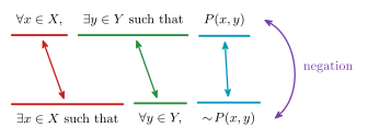
Figure 6: Negating a two-quantifier statement, piece by piece. The statement and its negation are stacked and aligned part-for-part, and each coloured pair shows one substitution: every ‘for all’ becomes a ‘there exists’ and picks up the words ‘such that’, every ‘there exists’ becomes a ‘for all’ and picks up the comma, and the predicate at the end is negated. Nothing changes order — \(x\) is still chosen before \(y\) in both rows, which is why the negation of a for-all-then-exists statement is an exists-then-for-all statement and not the other way round.
Two things the picture makes hard to get wrong. The “such that” travels with the \(\exists\), so it moves from the middle of the top row to the front of the bottom row and the comma moves the other way — that is punctuation, not content, but the course expects it. And the order of the variables does not move: the negation of a \(\forall\exists\) statement is an \(\exists\forall\) statement, never \(\forall\exists\) again, and never with \(x\) and \(y\) swapped.
Worked: negate, and determine truth
| Statement | Negation | Which is true | |
|---|---|---|---|
| (a) | \(\forall x \in \mathbb{R}, \exists y \in \mathbb{R}\) s.t. \(x + y = 0\) | \(\exists x \in \mathbb{R}\) s.t. \(\forall y \in \mathbb{R}, x + y \neq 0\) | original |
| (b) | \(\forall x \in \mathbb{R}, \exists y \in \mathbb{R}\) s.t. \(xy = 1\) | \(\exists x \in \mathbb{R}\) s.t. \(\forall y \in \mathbb{R}, xy \neq 1\) | negation |
| (c) | \(\exists x \in \mathbb{R}\) s.t. \(\forall y \in \mathbb{R}, xy = 0\) | \(\forall x \in \mathbb{R}, \exists y \in \mathbb{R}\) s.t. \(xy \neq 0\) | original |
- Given any \(x \in \mathbb{R}\), take \(y = -x\); then \(x + y = x + (-x) = 0\).
- Let \(x = 0\). Then \(0 \cdot y = 0 \neq 1\) for any value of \(y\), so the original fails.
- Take \(x = 0\). Then \(0 \cdot y = 0\) for any \(y\).
Worked: true or false?
| Statement | Verdict | |
|---|---|---|
| (a) | \(\forall x \in \mathbb{Z}, \exists y \in \mathbb{Z}\) s.t. \(y = 2x\) | True. Given any \(x \in \mathbb{Z}\), take \(y = 2x\). |
| (b) | \(\forall x \in \mathbb{Z}, \exists y \in \mathbb{Z}\) s.t. \(x = 2y\) | False. Take \(x = 3\) (or any odd integer): \(3 = 2y\) needs \(y = \frac{3}{2} \notin \mathbb{Z}\). |
| (c) | \(\forall x \in \mathbb{Z}, \exists y \in \mathbb{Z}\) s.t. \(y \geq x\) | True. Given any \(x \in \mathbb{Z}\), take \(y = x + 1\). |
| (d) | \(\exists x \in \mathbb{Z}\) s.t. \(\forall y \in \mathbb{Z}, xy = x\) | True. Take \(x = 0\); then \(0 \cdot y = 0\) for every \(y\). |
- and (b) look symmetric but aren’t — that asymmetry is the whole point of the ordering.
Worked: which statement is the negation?
Which one of the following is a negation of \(\forall x \in \mathbb{Z}, \exists y \in \mathbb{Z}\) such that \(x + y\) is odd?
- For every integer \(x\) there is an integer \(y\) such that \(x + y\) is not odd.
- There exists an integer \(x\) such that for every integer \(y\), \(x + y\) is odd. c. There exists an integer \(x\) such that \(x + y\) is even for every integer \(y\).
- For every integer \(x\) and every integer \(y\) there is an odd integer \(x + y\).
The negation is: \(\exists x \in \mathbb{Z}\) such that \(\forall y \in \mathbb{Z}\), \(x + y\) is not odd — i.e. is even. Options a and d keep the leading \(\forall\); option b fails to negate the predicate.
Here the original is true (so the negation is false): given any \(x \in \mathbb{Z}\), if \(x\) is odd take \(y = 0\) so \(x + y = x\) is odd; if \(x\) is even take \(y = 1\) so \(x + y = x + 1\) is odd.
See also
- quantified-statements · logical-equivalence-laws
- 2026-08-06-quantified-statements — Lecture 5
- 2026-08-10-direct-proof-and-counterexample — Lecture 7
- practice-problems — §7 Negation of Quantified Statements, with full worked solutions
- practice-problems — §8 Statements with Multiple Quantifiers, with full worked solutions
Lecture 5 — Valid Arguments (cont’d), Quantified Statements
Pre-work: Video 006 (Quantified Statements). Finishes the validity material from 2026-08-03-valid-and-invalid-arguments, then opens the quantifier topic — see quantified-statements for the reference definitions and tables this lecture builds on.
Learning goals
- Apply the ideas from Lecture 4 to determine the validity of an argument, including looking for truth values that would demonstrate an argument is invalid.
- Gain fluency in translating quantified statements (English to/from symbolic form).
- Be able to determine if a quantified statement is true or false.
Common questions
What exactly is a predicate? A sentence with a finite number of variables that becomes a statement when particular values are assigned to the variables. Examples: \(x > 0\), “\(x\) divides \(y\)”.
What are the symbols for the common domains? \(\mathbb{R}\) (real), \(\mathbb{Q}\) (rational), \(\overline{\mathbb{Q}}\) (irrational), \(\mathbb{Z}\) (integer), \(\mathbb{N}\) (natural). Written out in full:
\[\mathbb{Z} = \{\dots, -2, -1, 0, 1, 2, \dots\} \qquad \mathbb{Z}^{+} = \{1, 2, 3, \dots\}\]
\[\mathbb{Z}^{\text{even}} = \{\dots, -4, -2, 0, 2, 4, \dots\} \qquad \mathbb{Z}^{\text{nonneg}} = \{0, 1, 2, 3, \dots\} = \mathbb{Z}^{\geq 0}\]
The one to be careful with is \(\mathbb{N}\): both \(\mathbb{N} = \{0,1,2,\dots\}\) and \(\mathbb{N} = \{1,2,3,\dots\}\) are in use, and the ambiguity is not settled. Prefer \(\mathbb{Z}^{\geq 0}\) or \(\mathbb{Z}^+\) when you need to be unambiguous. The nesting diagram for these sets is in quantified-statements, and the fuller domains table is there too.
Worked: determining validity of a four-premise argument
If new messages are queued, then the file system is locked. The file system is not locked if and only if the system is functioning normally. New messages will not be sent to the message buffer only if they are queued. New messages will not be sent to the message buffer. Hence the system is not functioning normally.
Let \(p\) = “the file system is locked”, \(q\) = “new messages are queued”, \(r\) = “the system is functioning normally”, \(s\) = “new messages will be sent to the message buffer”.
The third premise is the awkward one. “\(a\) only if \(b\)” means \(\sim b \to \sim a\), which is equivalent to \(a \to b\) — so “\(\sim s\) only if \(q\)” becomes \(\sim s \to q\). (Recall from conditional-statements that in \(a \to b\), \(a\) is sufficient for \(b\) and \(b\) is necessary for \(a\).)
Symbolically:
- \(q \to p\)
- \(\sim p \leftrightarrow r\)
- \(\sim s \to q\)
- \(\sim s\)
\(\therefore \sim r\)
Solution 1 — assume the conclusion is false and the premises are true
Suppose all the premises are true but the conclusion is false.
- Conclusion false \(\Rightarrow\) \(r\) is true.
- Premise 4 is true \(\Rightarrow\) \(s\) is false.
- Premise 2 is true and \(r\) is true \(\Rightarrow\) \(\sim p\) is true, thus \(p\) is false.
- Premise 1 is true and \(p\) is false \(\Rightarrow\) \(q\) is false.
But now \(s\) is false (so \(\sim s\) is true) and \(q\) is false, which makes premise 3 (\(\sim s \to q\)) false. It is impossible to make all the premises true and the conclusion false, so the argument is valid.
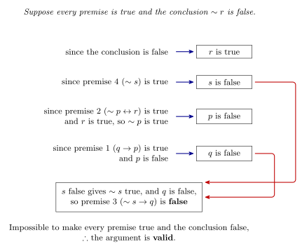
Figure 7: The search for an invalid row, and why it fails. Assuming the conclusion false fixes r, and each premise in turn is then forced to a single truth value with no choice left anywhere — until the last two forced values make premise 3 false, contradicting the assumption that every premise was true. No row can make the premises true and the conclusion false, so the argument is valid.
Every step above had only one value the premise permitted, so the search never branched. When a step does leave a choice open, both branches have to be followed — and a branch that survives to the end is exactly the row that shows the argument invalid.
Solution 2 — rules of inference and laws of logical equivalence
Goal: \(\sim r\).
- \(q \to p\) (premise)
- \(\sim p \leftrightarrow r\) (premise)
- \(\sim s \to q\) (premise)
- \(\sim s\) (premise)
- \(q\) — from 3 and 4 by Modus Ponens
- \(p\) — from 1 and 5 by Modus Ponens
- \((\sim p \to r) \land (r \to \sim p)\) — by definition of \(\leftrightarrow\), from 2
- \(r \to \sim p\) — from 7 by Specialization
- \(\sim r\) — from 6 and 8 by Modus Tollens (and double negation) \(\blacksquare\)
Line 9 can also be reached directly from 6 and 2 by the definition of \(\leftrightarrow\) plus double negation. See valid-argument-forms for the inference rules and determining-argument-validity for more worked comparisons of the two methods.
Quantified statements
| Symbol | Means | Associated English words |
|---|---|---|
| \(\forall\) | “for all” | all, every, any, each, none, no |
| \(\exists\) | “there exists” | there is, some, at least one, not all |
\(\in\) reads “belongs to” / “is an element of”; \(\notin\) reads “is not an element of”. The punctuation is part of the notation: \(\forall\) takes a comma, \(\exists\) takes the words “such that” (abbreviated s.t.).
| English | Symbolic |
|---|---|
| Every rational number is a real number. | \(\forall x \in \mathbb{Q}, x \in \mathbb{R}\) |
| No integer is an irrational number. | \(\forall x \in \mathbb{Z}, x \notin \overline{\mathbb{Q}}\) |
| Some real numbers are rational. | \(\exists x \in \mathbb{R}\) such that \(x \in \mathbb{Q}\) |
| Not all rational numbers are integers. | \(\exists x \in \mathbb{Q}\) such that \(x \notin \mathbb{Z}\) |
The English word does not hand you the symbol: “no”/“none” is universal, becoming \(\forall\) with the predicate negated, while “not all” is existential.
Sometimes you have to work out the quantifier from the context of the English sentence. “If an integer is a square, then it is nonnegative” names no quantifier at all, but it is a \(\forall\) statement:
\[\forall n \in \mathbb{Z}, \text{ if } n \text{ is a square, then } n \geq 0.\]
The full domains table and the negation rules are collected in quantified-statements.
Q3 from the pre-class questions
True or false? \(\exists y \in \mathbb{Z}\) such that \(y^2 - y = 0\).
The statement is true. Within the integers there is an integer for which \(y^2 - y = 0\) — choose \(y = 0\) or \(y = 1\). An existential statement only asks for one witness, so using only the numbers that make it true is allowed, and it does not matter that \(y = 2\) fails. The universal version, \(\forall y \in \mathbb{Z}, y^2 - y = 0\), is false — and \(y = 2\) is precisely what shows that.
Q4 from the pre-class questions — a universal quantified statement
True or false? \(\forall x \in \mathbb{Z}\), if \(6\) is divisible by \(x\), then \(x = 2\).
False. Consider \(x = 3\): we have \(3 \in \mathbb{Z}\), and \(6\) is divisible by \(3\), but \(3 \neq 2\). (Recall \(\sim(p \to q) \equiv p \land \sim q\) — a counterexample needs the hypothesis true and the conclusion false.)
The corrected statement is true: \(\forall x \in \mathbb{Z}\), if \(6\) is divisible by \(x\), then \(x = \pm 1\) or \(\pm 2\) or \(\pm 3\) or \(\pm 6\).
Worked: English to symbolic form
Translate, and determine truth. For (c), let \(P\) be the set of all prime numbers.
| Statement | Symbolic | T/F | Why | |
|---|---|---|---|---|
| (a) | There is a real number that is also an integer. | \(\exists x \in \mathbb{R}\) s.t. \(x \in \mathbb{Z}\) | T | take \(x = 1\) |
| (b) | If a real number is an integer, then it is a rational number. | \(\forall x \in \mathbb{R}\), if \(x \in \mathbb{Z}\) then \(x \in \mathbb{Q}\) | T | \(\mathbb{Z} \subseteq \mathbb{Q}\) |
| (c) | All prime numbers are odd. | \(\forall x \in P, x\) is odd | F | \(x = 2\) is prime but even |
| (d) | If an integer is divisible by 2 then it is divisible by 4. | \(\forall x \in \mathbb{Z}\), if \(2 \mid x\) then \(4 \mid x\) | F | \(x = 2\): \(2 \mid 2\) but \(4 \nmid 2\) |
Two notational points: \(2 \mid 6\) is read “2 divides 6” and is a statement, not a number (see divisibility-and-factorisation); and \(\{\mathbb{Z}\} \neq \mathbb{Z}\), so writing \(x \in \{\mathbb{Z}\}\) would say \(x\) is the set of integers.
Worked: symbolic to English
| Statement | English | T/F | Why | |
|---|---|---|---|---|
| (a) | \(\exists x \in \mathbb{R}\) s.t. \(x^2 = 2\) | There is a real number whose square is 2. | T | \(x = \sqrt{2}\) |
| (b) | \(\forall x \in \{1,2,3,4,5\}, x\) is prime | Every integer from 1 to 5 is prime. | F | \(1\) is not prime |
| (c) | \(\exists x \in \{1,2,3,4,5\}\) s.t. \(x > 4\) | Some integer from 1 to 5 is greater than 4. | T | take \(x = 5 > 4\) |
| (d) | \(\forall x \in \mathbb{R}\), if \(x^3 < 8\) then \(x < 2\) | If the cube of a real number is less than 8 then it is less than 2. | T | see Figure 8 |
| (e) | \(\forall x \in \mathbb{R}, (x > 0\) or \(x < 0)\) | Every real number is positive or negative. | F | \(x = 0\) is neither positive nor negative |
One counterexample is enough for (b). Both \(x = 1\) and \(x = 4\) work, but \(1\) is the more instructive one: it is neither prime nor composite, which is the trap that comes back in 2026-08-06-negation-and-multiple-quantifiers.
For (d), the graph of \(y = x^3\) shows why:
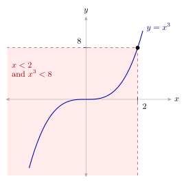
Figure 8: Why ‘if \(x^3 < 8\) then \(x < 2\)’ is true. The cube function is increasing and passes through \((2,8)\), so the whole of the curve to the left of \(x=2\) lies below \(y=8\) and none of the curve to the right does — the two conditions cut the curve at the same place.
Compare (d) with (d) of the English-to-symbolic table above, \(\forall x \in \mathbb{Z}\), if \(2 \mid x\) then \(4 \mid x\), which is false: a universal conditional needs the implication to hold at every point of the domain, and one \(x\) where the hypothesis holds and the conclusion fails sinks it.
See also
- quantified-statements · valid-argument-forms · determining-argument-validity
- 2026-08-06-negation-and-multiple-quantifiers — Lecture 6
- practice-problems — §6 Quantified Statements, with full worked solutions
Week 3
Lecture 7 — Direct Proof, Counterexample
Pre-work: Video 009 (Direct Proofs and Counterexamples). First lecture of the number theory and methods of proof topic — see proof-techniques for the reference definitions, proof templates and the catalogue of common proof errors.
Learning goals
- How to write a direct proof.
- How to disprove a statement by exhibiting a counterexample.
Definitions to know
Proofs and disproofs need the precise definitions of even, odd, prime, composite, rational, divides, … Each of the six below is a biconditional, because a proof reads a definition in both directions: unfolding it in the hypothesis, and folding it back up in the conclusion.
| \(n\) is an even integer | \(\leftrightarrow\) | \(n = 2k\) for some integer \(k\) |
| \(n\) is an odd integer | \(\leftrightarrow\) | \(n = 2k + 1\) for some integer \(k\) |
| \(n\) is a prime number | \(\leftrightarrow\) | \(n \in \mathbb{Z}\), \(n > 1\), and \(\forall r, s \in \mathbb{Z}^{+}\), if \(n = rs\) then (\(r = 1\) and \(s = n\)) or (\(r = n\) and \(s = 1\)) |
| \(n\) is a composite number | \(\leftrightarrow\) | \(n \in \mathbb{Z}\), \(n > 1\), and \(\exists r, s \in \mathbb{Z}^{+}\) such that \(n = rs\) and \(1 < r < n\) and \(1 < s < n\) |
| \(r\) is a rational number | \(\leftrightarrow\) | \(\exists a, b \in \mathbb{Z}\) such that \(r = \frac{a}{b}\) and \(b \neq 0\) |
| \(d \mid n\) | \(\leftrightarrow\) | \(d \neq 0\) and \(n = dk\) for some integer \(k\) |
Two points about these definitions:
- “Odd” has a second, equally valid form. \(n = 2k + 1\) for some integer \(k\) and \(n = 2k - 1\) for some integer \(k\) are equivalent: they define the same set, and you may finish a proof in whichever form drops out of the algebra. The proof that \(\frac{x}{2}\) is odd, below, is where it pays off: it lands on the \(2k - 1\) form.
- The \(b \neq 0\) in the definition of rational is its own requirement, separate from \(r = \frac{a}{b}\). A “rational” claim is two claims: that the fraction exists, and that its denominator is non-zero. Dropping the second half is the standard way to lose the mark — see rational-and-irrational-numbers.
How much detail to give in a proof. Demonstrate facts using the definitions. That is the whole answer, and it is why the definitions come first.
Two facts, and where “not prime” bites
Fact: the sum, difference, and product of integers is an integer.
Fact: every integer is either even or odd.
The first is what licenses lines like “since \(k \in \mathbb{Z}\), we have \(3k + 2 \in \mathbb{Z}\)” — cheap, but it has to be said, because the definition of odd demands an integer witness and nothing else supplies it.
What “not prime” means. For \(n \in \mathbb{Z}^{>1}\), “\(n\) is not prime” means “\(n\) is composite”. For \(n \in \mathbb{Z}\) generally, “\(n\) is not prime” means “composite or \(n \leq 1\)”. Primality and compositeness only carve up the integers from \(2\) upwards; \(1\), \(0\) and the negatives are in neither class.
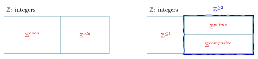
Figure 9: Two ways of splitting \(\mathbb{Z}\). Left: even and odd exhaust the integers, which is what makes ‘every integer is either even or odd’ usable as a case split. Right: prime and composite do not — they only partition \(\mathbb{Z}^{\geq 2}\), and everything from \(1\) downwards falls in \(\mathbb{Z}^{\leq 1}\). The heavy blue box round the two right-hand cells marks \(\mathbb{Z}^{\geq 2}\), the same restriction as \(\mathbb{Z}^{>1}\).
The asymmetry between the two panels is the point. The left one is a genuine two-case split you may argue by; the right one is not, and a proof that reasons “\(n\) is not prime, so \(n\) is composite” is only sound once \(n \geq 2\) has been established. The proof about \(n^2 + 5n + 6\) below turns on exactly that.
Proof or disproof of \(\forall x \in D, P(x) \to Q(x)\)
Every method in this topic attacks one row of the truth table for \(p \to q\): the only row that makes it false is \(p\) true, \(q\) false.
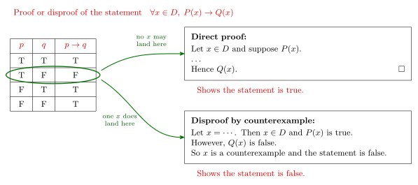
Figure 10: The truth table for \(p \to q\) beside the skeletons of a direct proof and a disproof by counterexample. The green ring marks the T-F-F row: it is the only row that can make \(P(x) \to Q(x)\) false, so it is the only row either method has to deal with. A direct proof shows no \(x \in D\) can land there; a counterexample exhibits one \(x\) that does. The two green arrows join that row to the two skeletons.
Why a direct proof supposes \(P(x)\) is true. \(P(x) \to Q(x)\) would still be true if \(P(x)\) is false, so that case needs no argument. We just need to rule out the case that \(P(x)\) is true and \(Q(x)\) is false — so we suppose \(P(x)\) is true and prove that in this case \(Q(x)\) must also be true. The other three rows of the table are true for free, so there is nothing to do in them.
The mirror image is what makes a counterexample work: because the statement fails as soon as one \(x\) occupies that row, exhibiting one such \(x\) is a complete disproof. See conditional-statements for the truth table itself.
Worked: which values give a counterexample? (pre-class Q1)
Which values for \(m\) and \(n\) give a counterexample disproving: for all integers \(m\) and \(n\), if \(2m + n\) is odd, then \(m\) and \(n\) are both odd?
| Check | Verdict | |
|---|---|---|
| a. \(m = 3, n = 5\) | \(2(3) + 5 = 11\) odd, but \(m, n\) are both odd — so \(q\) is true | not a counterexample |
| b. \(m = 3, n = 6\) | \(2(3) + 6 = 12\) even — so \(p\) is false | not a counterexample |
| c. \(m = 4, n = 5\) | \(2(4) + 5 = 13\) odd, and \(m, n\) are not both odd (at least one is even) | counterexample |
| d. \(m = 4, n = 6\) | \(2(4) + 6 = 14\) even — so \(p\) is false | not a counterexample |
For a counterexample to \(p \to q\) we require \(p\) true and \(q\) false. Options (b) and (d) fail for the opposite reason to (a): they never even engage the statement, because a conditional with a false hypothesis is true and so proves nothing either way.
The wording for (c) matters: not “\(m\) and \(n\) are both even”, but “not both \(m, n\) are odd — at least one is even”. Negating “both odd” gives “at least one is even”, not “both even”. That is the De Morgan step this question is testing. See 2026-08-06-negation-and-multiple-quantifiers.
Example proof
\(\forall n \in \mathbb{Z}\), if \(n\) is odd then \(3n + 2\) is odd.
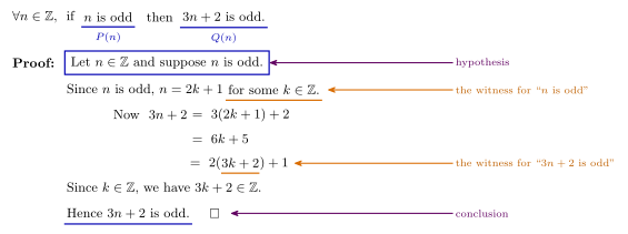
Figure 11: The anatomy of a direct proof. The opening line is boxed, the purple margin labels mark the hypothesis and the conclusion, and the orange underlines and margin captions mark the two integer witnesses. The blue underlines on the statement pick out its two halves, \(P(n)\) and \(Q(n)\), which ties the proof back to the skeleton above.
The shape to memorise:
- State the hypothesis in the skeleton’s words —
Let n ∈ ℤ and suppose n is odd. - Unfold the definition, naming a witness: \(n = 2k + 1\) for some \(k \in \mathbb{Z}\).
- Do the algebra until the target definition is visible — \(6k + 5\) is not obviously odd; \(2(3k+2) + 1\) is, because it matches the shape \(2(\text{integer}) + 1\) exactly.
- Confirm the new witness is an integer, by the Fact above.
- State the conclusion in the target’s own words.
Step 4 is the one most often skipped. \(2(3k+2)+1\) only certifies “odd” if \(3k+2\) is an integer, and saying so costs one line.
Worked: if \(x + 6 = 4y\) then \(\frac{x}{2}\) is odd
For any integer \(x\), if \(x + 6 = 4y\) for some integer \(y\), then \(\frac{x}{2}\) is an odd integer.
Proof. Let \(x \in \mathbb{Z}\) and suppose \(x + 6 = 4y\) for some \(y \in \mathbb{Z}\). Now \(x = 4y - 6\), so \(x = 2(2y - 3)\). Hence \(\dfrac{x}{2} = \dfrac{2(2y-3)}{2} = 2y - 3 = 2(y-1) - 1\). Thus, because \(y \in \mathbb{Z}\), we have \(2y - 3 \in \mathbb{Z}\) so \(\frac{x}{2} \in \mathbb{Z}\); and \(y - 1 \in \mathbb{Z}\), so by definition \(\frac{x}{2}\) is odd. \(\square\)
Three things this proof drills:
- The hypothesis is itself existential. “\(x + 6 = 4y\) for some integer \(y\)” hands you a \(y\); the opening line accepts it by name and the rest of the proof uses it.
- The conclusion is a conjunction, and both halves need discharging. \(\frac{x}{2}\) must be shown to be an integer (via \(2y - 3 \in \mathbb{Z}\)) and to have the odd form. Neither half implies the other.
- Either form of “odd” finishes it. The proof ends on \(2(y-1) - 1\), and \(2(y-2) + 1\) does just as well. This is the \(n = 2k - 1\) equivalence from the definitions, cashed in.
Worked: prove or disprove
The primes begin \(2, 3, 5, 7, 11, \dots\)
(a) There are distinct integers \(m\) and \(n\) such that \(\frac{1}{m} + \frac{1}{n}\) is an integer.
True. Take \(m = 1\) and \(n = -1\). Then \(\frac{1}{m} + \frac{1}{n} = 1 + (-1) = 0 \in \mathbb{Z}\).
The statement is existential, so one witness is the proof — the opposite of the situation with \(n^2 + 5n + 6\) below. The word distinct matters: it rules out the easy \(m = n = 1\), so the witness uses a negative integer instead.
(b) \(\forall n \in \mathbb{Z}^{\geq 2}\), \(n\) is composite or \(n + 1\) is composite.
False. Take \(n = 2\): then \(n = 2\) and \(n + 1 = 3\), which are both prime.
This one is a universal statement that is not a conditional — the predicate is a disjunction. So the counterexample has to falsify the disjunction outright, i.e. make both disjuncts false, which here means finding two consecutive primes. \(n = 2\) is the only value that works, because for \(n \geq 3\) one of \(n\), \(n+1\) is even and bigger than \(2\), hence composite.
(c) For each integer \(n \geq 2\), the product of the first \(n\) prime numbers minus 1 is prime.
False. Try \(n = 2, 3, 4, \dots\) in turn. Take \(n = 4\):
\[2 \cdot 3 \cdot 5 \cdot 7 - 1 = 209 = 11 \cdot 19 \quad\text{— composite.}\]
The two values before it: \(n = 2\) gives \(2 \cdot 3 - 1 = 5\), prime; \(n = 3\) gives \(2 \cdot 3 \cdot 5 - 1 = 29\), prime. So the first two cases both hold and the claim only breaks at the third. That is why “arguing from examples” is on the list of common proof errors in proof-techniques. A pattern surviving two checks is not evidence of anything.
Worked: disprove by proving the negation
Show that \(\exists n \in \mathbb{Z}^{+}\) such that \(n^2 + 5n + 6\) is prime is false, by proving the negation.
The statement is existential, so a counterexample won’t do — one bad \(n\) says nothing about whether some other \(n\) works. Negating it turns it into a universal, and that has to be proved outright:
Negation: \(\forall n \in \mathbb{Z}^{+}\), \(n^2 + 5n + 6\) is composite.
Proof of the negation. Let \(n \in \mathbb{Z}^{+}\). Now \(n^2 + 5n + 6 = (n+2)(n+3)\). Since \(n \geq 1\) we have \(n + 2 > 1\) and \(n + 3 > 1\). Thus \(n^2 + 5n + 6\) is composite. \(\square\)
The original statement is false (F) and its negation is true (T). The step from “not prime” to “composite” needs a justification: because \(n \geq 1\) we have \(n^2 + 5n + 6 \geq 2\), so “not prime” is “composite”. The value sits in \(\mathbb{Z}^{\geq 2}\), the region of Figure 9 where the two really do coincide. Without that check the negation of “prime” would also have to admit values \(\leq 1\).
One small gap to close: the proof gives only the two “\(> 1\)” halves, but the definition of composite asks for factors with \(1 < r < n\) and \(1 < s < n\). Here each factor is also strictly less than the product, since the other factor exceeds \(1\) — so \(n+2 < (n+2)(n+3)\) and \(n+3 < (n+2)(n+3)\), and the definition is met in full.
The general move — to disprove \(\exists x \in D\) such that \(P(x)\), prove \(\forall x \in D, \sim P(x)\) — is the quantifier negation rule from 2026-08-06-negation-and-multiple-quantifiers used as a proof strategy. It generalises: a universal falls to one counterexample, an existential needs a universal proof.
See also
- proof-techniques · quantified-statements · conditional-statements
- rational-and-irrational-numbers · divisibility-and-factorisation — the two definitions from the table that get their own notes
- 2026-08-13-proof-by-contradiction — Lecture 8, which adds a third skeleton to the two above
- 2026-08-13-proof-by-contraposition — Lecture 9, which adds the fourth
- math1061-diagram-notation — the house conventions the figures above follow
- practice-problems — §9 Direct Proofs and Counterexamples, with full worked solutions
Lecture 8 — Proof by Contradiction
Pre-work: Video 010 (Proof by Contradiction). Adds a third method to the direct proof and counterexample of 2026-08-10-direct-proof-and-counterexample — see proof-techniques for all four side by side.
Learning goals
- How to write a proof by contradiction.
Recall
The negations this method depends on (see logical-equivalence-laws and quantified-statements):
\[\sim(p \lor q) \equiv \sim p \land \sim q\] \[\sim(p \land q) \equiv \sim p \lor \sim q\] \[\sim(p \to q) \equiv p \land \sim q\] \[\sim\big(\exists x \in D \text{ such that } P(x)\big) \equiv \forall x \in D, \sim P(x)\] \[\sim\big(\forall x \in D, P(x)\big) \equiv \exists x \in D \text{ such that } \sim P(x)\]
The definitions every proof below unfolds
The definitions are written as biconditionals, because a proof uses them in both directions — read left-to-right to unpack a hypothesis, right-to-left to establish a conclusion.
- \(n\) is an even integer \(\leftrightarrow\) \(n = 2k\) for some integer \(k\)
- \(n\) is an odd integer \(\leftrightarrow\) \(n = 2k+1\) for some integer \(k\) \(\;\leftrightarrow\;\) \(n = 2k-1\) for some integer \(k\)
- \(n\) is a prime number \(\leftrightarrow\) \(n \in \mathbb{Z}\), \(n > 1\), and \(\forall r,s \in \mathbb{Z}^+\), if \(n = rs\) then (\(r = 1\) and \(s = n\)) or (\(r = n\) and \(s = 1\))
- \(n\) is a composite number \(\leftrightarrow\) \(n \in \mathbb{Z}\), \(n > 1\), and \(\exists r,s \in \mathbb{Z}^+\) such that \(n = rs\) and \(1 < r < n\) and \(1 < s < n\)
- \(r\) is a rational number \(\leftrightarrow\) \(\exists a, b \in \mathbb{Z}\) such that \(r = \frac{a}{b}\) and \(b \neq 0\)
- \(d \mid n \leftrightarrow d \neq 0\) and \(n = dk\) for some integer \(k\)
Both forms of “odd” are usable: \(2k+1\) and \(2k-1\) describe the same set of integers, and some calculations come out tidier with one than the other. The same definitions are tabulated in proof-techniques; the rational one is unpacked in rational-and-irrational-numbers and the divisibility one in divisibility-and-factorisation.
Fact: the sum, difference and product of integers is an integer.
Warning: don’t assume something that seems like an “obvious fact” until you have proven it, or can say which lecture or pre-work video it was proved in.
When to use contradiction
Three questions share one answer: whether proof by contradiction can be used for every proof, whether it only works for universal statements or just works best for them, and which situations suit it over a direct proof. Proof by contradiction is the most versatile method, but it requires more set-up, so sometimes a direct proof is easier.
Proof by counterexample and proof by contradiction do opposite jobs. Counterexample is a disproof; contradiction is a proof.
The three methods so far
There are three proof skeletons so far (Figure 12); the fourth arrives next lecture.
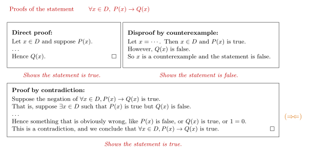
Figure 12: Three proof skeletons for the same statement, each with its verdict in red underneath. Only the contradiction box starts by assuming the statement false; the other two start from the statement’s own hypothesis. The orange \((\Rightarrow\Leftarrow)\) in the margin marks the point where the contradiction lands.
For a proof by contradiction we begin by assuming that the statement is false — equivalently, that the negation of the statement is true. The negation of \(\forall x \in D, P(x) \to Q(x)\) is
\[\exists x \in D \text{ such that } P(x) \land \sim Q(x)\]
and we derive from it something that cannot hold — \(P(x)\) false, or \(Q(x)\) true, or \(1 = 0\).
Note what the two moves in that negation are: the \(\forall\) becomes an \(\exists\) (so you are handed one specific \(x\) to work with, not an arbitrary one), and \(\sim(P \to Q) \equiv P \land \sim Q\) turns the implication into a conjunction (so you get to assume the hypothesis and the failure of the conclusion at once). Both extra assumptions are why the method is the most versatile one, and why it costs more set-up.
The contradiction mark. \((\Rightarrow\Leftarrow)\) — two arrows meeting head-on — is written inline at the point where the contradiction lands. Every proof by contradiction below uses it. It is a marker, not a substitute for saying in words what contradicts what.
Worked: how to start a proof by contradiction
Claim: \(\forall n \in \mathbb{Z}\), if \(n\) is odd then \(3n+2\) is odd. An appropriate way to start a proof by contradiction is:
Proof: Suppose that \(n\) is an odd integer and that \(3n + 2\) is even.
which means exactly the same thing as
Suppose \(\exists n \in \mathbb{Z}\) such that \(n\) is odd but \(3n + 2\) is even.
The second phrasing is the one the negation rule actually produces, so it is the safer one to write while you are learning; the first is the same sentence with the existential left implicit.
Worked: what type of proof starts this way?
Claim: for all integers \(m\) and \(n\), if \(mn\) is even, then \(m\) is even or \(n\) is even. Consider the first sentence of a proof:
Proof: Suppose that \(m\) and \(n\) are integers, \(mn\) is even and both \(m\) and \(n\) are odd.
This is the start of a proof by contradiction, not a direct proof and not a disproof by counterexample. It assumes the hypothesis and the negation of the conclusion (“\(m\) even or \(n\) even” negates to “\(m\) odd and \(n\) odd” by De Morgan).
Worked: the same statement, both ways
\(\forall n \in \mathbb{Z}\), if \(n\) is odd then \(3n + 2\) is odd.
It can be proved both ways (Figure 13).
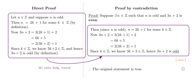
Figure 13: The same statement proved both ways — direct proof left, proof by contradiction right. The purple outline marks the body the two proofs share, and the arrow carries it across: it is character-for-character the same algebra. Contradiction only adds an assumption line on top and the \((\Rightarrow\Leftarrow)\) plus conclusion at the bottom. That extra wrapper is the ‘more set-up’ that contradiction costs.
Direct proof
Let \(n \in \mathbb{Z}\) and suppose \(n\) is odd. Then \(n = 2k+1\) for some \(k \in \mathbb{Z}\) (by definition). Now \[3n + 2 = 3(2k+1) + 2 = 6k + 5 = 2(3k+2) + 1.\] Since \(k \in \mathbb{Z}\), we know \(3k + 2 \in \mathbb{Z}\), and hence \(3n+2\) is odd (by definition). \(\square\)
Proof by contradiction
Suppose \(\exists n \in \mathbb{Z}\) such that \(n\) is odd and \(3n + 2\) is even. Then (since \(n\) is odd), \(n = 2k+1\) for some \(k \in \mathbb{Z}\). Now \[3n + 2 = 3(2k+1) + 2 = 6k + 5 = 2(3k+2) + 1.\] Since \(k \in \mathbb{Z}\), we know \(3k+2 \in \mathbb{Z}\), hence \(3n+2\) is odd \((\Rightarrow\Leftarrow)\) — contradicting the assumption that it is even. Therefore the original statement is true. \(\square\)
The body of the two proofs is identical; contradiction just wraps it in an extra assumption and an extra closing line. That’s the “more set-up” cost — and here the direct proof is the better choice.
Worked: where contradiction earns its keep
\(\forall m, n \in \mathbb{Z}\), if \(mn\) is even, then \(m\) is even or \(n\) is even.
Direct proof — suppose \(m, n \in \mathbb{Z}\) and \(mn\) is even. We can write \(mn = 2k\) for some \(k \in \mathbb{Z}\) … and now there’s no way forward: knowing \(mn = 2k\) tells you nothing about \(m\) and \(n\) individually.
Proof by contradiction
Suppose \(\exists m, n \in \mathbb{Z}\) such that \(mn\) is even and both \(m\) and \(n\) are odd. Since \(m\) is odd, \(m = 2k+1\) for some \(k \in \mathbb{Z}\). Since \(n\) is odd, \(n = 2\ell + 1\) for some \(\ell \in \mathbb{Z}\) — use a new variable; \(m\) and \(n\) need not be equal. Now \[mn = (2k+1)(2\ell+1) = 4k\ell + 2k + 2\ell + 1 = 2(2k\ell + k + \ell) + 1.\] Since \(k, \ell \in \mathbb{Z}\), \(2k\ell + k + \ell \in \mathbb{Z}\), so \(mn\) is odd. It is impossible for \(mn\) to be both even and odd \((\Rightarrow\Leftarrow)\). Therefore the original statement is true. \(\square\)
Reusing \(k\) for both \(m\) and \(n\) is one of the standard proof errors listed in proof-techniques. Note also where the contradiction lands here: not on a stray arithmetic absurdity but on the hypothesis itself — the assumed-even \(mn\) turns out to be odd. That is one of the three landing points listed above (“\(P(x)\) is false”).
Worked: if \(3n^3 - 2\) is odd then \(n\) is odd
Prove by contradiction: \(\forall n \in \mathbb{Z}\), if \(3n^3 - 2\) is odd, then \(n\) is odd.
Proof. Suppose the statement is false. That means \(\exists n \in \mathbb{Z}\) such that \(3n^3 - 2\) is odd and \(n\) is even. Since \(n\) is even, \(n = 2a\) for some \(a \in \mathbb{Z}\). Now \[3n^3 - 2 = 3(2a)^3 - 2 = 3 \cdot 8a^3 - 2 = 24a^3 - 2 = 2(12a^3 - 1).\] Since \(a \in \mathbb{Z}\), \(12a^3 - 1 \in \mathbb{Z}\), so \(3n^3 - 2\) is even \((\Rightarrow\Leftarrow)\) — a contradiction. Therefore the original statement is true. \(\square\)
The negation is worth reading slowly: “if \(3n^3-2\) is odd then \(n\) is odd” negates to “\(3n^3 - 2\) is odd and \(n\) is even”. The even hypothesis is the one that gives you something to substitute, so that is where the work starts.
Worked: without loss of generality
\(\forall m, n \in \mathbb{Z}\), if \(m + n\) is even, then \(m\) and \(n\) are both even or \(m\) and \(n\) are both odd.
Proof. Suppose the statement is false. Thus \(\exists m, n \in \mathbb{Z}\) such that \(m + n\) is even but exactly one of \(m, n\) is even (and the other is odd).
Without loss of generality (WLOG), assume \(m\) is even and \(n\) is odd. (The two cases are (1) \(m\) even, \(n\) odd and (2) \(m\) odd, \(n\) even; since \(m + n = n + m\), the second is the first with the names swapped, so proving one proves both.)
Thus \(m = 2a\) for some \(a \in \mathbb{Z}\), and \(n = 2b + 1\) for some \(b \in \mathbb{Z}\). Now \[m + n = (2a) + (2b+1) = 2(a+b) + 1.\] We know \(a + b \in \mathbb{Z}\) because \(a, b \in \mathbb{Z}\), so \(m + n\) is odd. This contradicts the assumption that \(m + n\) is even \((\Rightarrow\Leftarrow)\). Therefore the original statement is true. \(\square\)
“Without loss of generality” is only legitimate when the omitted case really is the stated one relabelled — say why, as above. The phrase abbreviates to WLOG.
See also
- proof-techniques · quantified-statements · logical-equivalence-laws
- 2026-08-13-proof-by-contraposition — Lecture 9
- practice-problems — §10 Proof by Contradiction, with full worked solutions
Lecture 9 — Proof by Contraposition, Rational Numbers
Pre-work: Video 011 (Proof by Contraposition), Video 012 (Rational Numbers). Completes the set of four methods — see proof-techniques for the full comparison, and rational-and-irrational-numbers for the \(\mathbb{Q}\) / \(\overline{\mathbb{Q}}\) definitions and closure results.
Learning goals
- Understand the definitions of rational and irrational numbers.
- Gain fluency in proof techniques (direct proof, proof by contradiction and proof by contraposition).
Recall: \(r \in \mathbb{Q} \iff r = \frac{a}{b}\) for some \(a, b \in \mathbb{Z}\) where \(b \neq 0\); and \(r \in \overline{\mathbb{Q}} \iff r \notin \mathbb{Q}\), where \(\overline{\mathbb{Q}} = \mathbb{R} \setminus \mathbb{Q}\). So \(\frac{3}{4} \in \mathbb{Q}\), while \(\sqrt{2} \in \overline{\mathbb{Q}}\) and \(\pi \in \overline{\mathbb{Q}}\). The barred \(\overline{\mathbb{Q}}\) is this course’s symbol for the irrationals — see rational-and-irrational-numbers for the picture.
The four methods
| Method | Shape | Shows |
|---|---|---|
| Direct proof | Let \(x \in D\) and suppose \(P(x)\). \(\dots\) Hence \(Q(x)\). | true |
| Disproof by counterexample | Let \(x = \cdots\). Then \(x \in D\) and \(P(x)\) is true. However \(Q(x)\) is false. | false |
| Proof by contradiction | Suppose \(\exists x \in D\) such that \(P(x)\) is true but \(Q(x)\) is false. \(\dots\) Hence something obviously wrong. | true |
| Proof by contraposition | We prove \(\forall x \in D, \sim Q(x) \to \sim P(x)\). Let \(x \in D\) and suppose \(\sim Q(x)\). \(\dots\) Hence \(\sim P(x)\). | true |
This is the table from 2026-08-13-proof-by-contradiction, grown by one row. Contraposition is valid because
\[p \to q \equiv \sim q \to \sim p\]
(see conditional-statements). Contraposition does not assume the statement is false. It is a direct proof of a different statement — one that happens to be logically equivalent to the one you were asked about. That is the practical difference from proof by contradiction, which assumes \(P(x) \land \sim Q(x)\) and hunts for an absurdity.
Choosing a method
What is the relationship between proof by contradiction and proof by contraposition? As above: contraposition is a direct proof of an equivalent statement, while contradiction assumes \(P(x) \land \sim Q(x)\) and hunts for an absurdity.
How do we decide if we should use a direct proof, proof by contradiction or proof by contraposition? Empirically rather than by a rule: for each statement, ask what type of proof will work, and see which methods move and which ones stall. The verdicts for the statements proved below are collected in Figure 14.
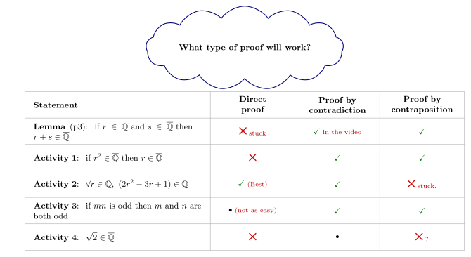
Figure 14: Which type of proof works for each statement proved below. A tick is a method that works and a cross is one that stalls, with a short remark in red where there is one; a plain bullet is a method given neither. Reading down the columns: contradiction is the only method never ruled out, which is what ‘most versatile’ means in practice — but it is also never the one labelled ‘Best’.
The pattern that emerges: a method works when it hands you something you can substitute for. A direct proof needs the hypothesis to be a positive, unfoldable statement; contraposition needs the negated conclusion to be one; contradiction gets both at once, which is why its column never gets a cross.
The last lemma from Video 12, by contraposition
Lemma: the sum of any rational number and any irrational number is irrational.
Symbolically, either of:
\[\forall r, s \in \mathbb{R}, \text{ if } r \in \mathbb{Q} \text{ and } s \in \overline{\mathbb{Q}} \text{ then } r + s \in \overline{\mathbb{Q}}\] \[\forall r \in \mathbb{Q} \text{ and } \forall s \in \mathbb{R}, \text{ if } s \in \overline{\mathbb{Q}} \text{ then } r + s \in \overline{\mathbb{Q}}\]
The second is the form to work with, because it puts the whole conditional in terms of one unknown \(s\): the antecedent is \(s \in \overline{\mathbb{Q}}\) and the consequent is \(r + s \in \overline{\mathbb{Q}}\), so the contrapositive is a clean swap.
- Direct proof: suppose \(r \in \mathbb{Q}\) and \(s \in \overline{\mathbb{Q}}\). Now we are stuck — \(s \in \overline{\mathbb{Q}}\) gives nothing to substitute.
- Proof by contradiction: suppose \(\exists r \in \mathbb{Q}\) and \(s \in \mathbb{R}\) such that \(s \in \overline{\mathbb{Q}}\) and \(r + s \in \mathbb{Q}\). (Worked in Video 012.)
- Proof by contraposition:
The contrapositive is: \(\forall r \in \mathbb{Q}\) and \(\forall s \in \mathbb{R}\), if \(r + s \in \mathbb{Q}\) then \(s \in \mathbb{Q}\).
Suppose \(r \in \mathbb{Q}\), \(s \in \mathbb{R}\) and \(r + s \in \mathbb{Q}\). Since \(r \in \mathbb{Q}\), \(r = \frac{a}{b}\) for some \(a, b \in \mathbb{Z}\) where \(b \neq 0\). Since \(r + s \in \mathbb{Q}\), \(r + s = \frac{c}{d}\) for some \(c, d \in \mathbb{Z}\) where \(d \neq 0\) — a new pair of variables, since nothing says the two fractions are related. Now \[s = (r+s) - r = \frac{c}{d} - \frac{a}{b} = \frac{bc - ad}{bd}.\] Since \(a,b,c,d \in \mathbb{Z}\) we know \(bc - ad \in \mathbb{Z}\) and \(bd \in \mathbb{Z}\). Also \(bd \neq 0\) since \(b \neq 0\) and \(d \neq 0\). Thus \(s \in \mathbb{Q}\). \(\square\)
The move that unlocks it is writing \(s = (r+s) - r\) — expressing the unknown in terms of the two things you were handed. The closing three checks (integer numerator, integer denominator, non-zero denominator) are what the definition of \(\mathbb{Q}\) actually demands, and every rational-number proof in this course ends with them.
Worked: if \(r^2\) is irrational then \(r\) is irrational
Prove that \(\forall r \in \mathbb{R}\), if \(r^2\) is irrational, then \(r\) is irrational.
Which type of proof will work: contradiction and contraposition both work; a direct proof does not.
Proof. We prove the contrapositive: \(\forall r \in \mathbb{R}\), if \(r \in \mathbb{Q}\) then \(r^2 \in \mathbb{Q}\). Suppose \(r \in \mathbb{R}\) where \(r \in \mathbb{Q}\). Then \(r = \frac{a}{b}\) for some integers \(a, b\) with \(b \neq 0\). Now \(r^2 = \left(\frac{a}{b}\right)^2 = \frac{a^2}{b^2}\). Since \(a, b \in \mathbb{Z}\) we have \(a^2, b^2 \in \mathbb{Z}\); also \(b^2 \neq 0\) since \(b \neq 0\). So \(r^2 \in \mathbb{Q}\). \(\square\)
Both negations do real work here. “\(r^2\) is irrational” is a statement about what \(r^2\) is not, and so is “\(r\) is irrational” — the contrapositive turns both into positive membership claims, and a positive claim is one you can substitute a fraction into.
Worked: \(2r^2 - 3r + 1\) is rational when \(r\) is
Prove that \(\forall r \in \mathbb{Q}, (2r^2 - 3r + 1) \in \mathbb{Q}\).
Which type of proof will work: a direct proof works and is the best; contradiction also works; contraposition gets stuck.
Proof. Let \(r \in \mathbb{Q}\). Then \(r = \frac{a}{b}\) for some \(a, b \in \mathbb{Z}\) where \(b \neq 0\). Now \[2r^2 - 3r + 1 = 2\left(\frac{a}{b}\right)^2 - 3\left(\frac{a}{b}\right) + 1 = \frac{2a^2}{b^2} - \frac{3ab}{b^2} + \frac{b^2}{b^2} = \frac{2a^2 - 3ab + b^2}{b^2}.\] Since \(a, b \in \mathbb{Z}\) we have \(2a^2 - 3ab + b^2 \in \mathbb{Z}\) and \(b^2 \in \mathbb{Z}\). Also \(b^2 \neq 0\) since \(b \neq 0\). So \(2r^2 - 3r + 1 \in \mathbb{Q}\). \(\square\)
In the middle step everything is put over the common denominator \(b^2\) before the numerator is inspected, so that the final expression is visibly one integer over one non-zero integer.
Contraposition stalls here because the negation of “\(2r^2 - 3r + 1 \in \mathbb{Q}\)” — that it’s irrational — gives nothing to substitute. The direction of the useful information decides the method.
Worked: if \(mn\) is odd then \(m\) and \(n\) are both odd
Prove by contraposition: \(\forall m, n \in \mathbb{Z}\), if \(mn\) is odd, then \(m\) and \(n\) are both odd.
Which type of proof will work: contradiction and contraposition both work; a direct proof is not as easy.
Label the two halves of the statement \(p\) and \(q\) first, and only then write the contrapositive underneath: forming a contrapositive is a mechanical two-step operation on those labelled parts, not a fresh piece of thinking (Figure 15).
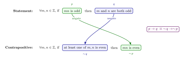
Figure 15: Forming the contrapositive of ‘if mn is odd then m and n are both odd’, with the parts labelled p and q. Two things happen at once and both are needed: each half is negated, and the two halves swap sides. The crossing arrows are what ‘swap’ looks like. The negation of q is the De Morgan step — ‘m and n are both odd’ becomes ‘at least one of m, n is even’ — which is where this kind of proof is most often got wrong.
Proof. We prove the contrapositive: \(\forall m, n \in \mathbb{Z}\), if at least one of \(m, n\) is even then \(mn\) is even. Without loss of generality, assume \(m\) is even. So \(m = 2k\) for some \(k \in \mathbb{Z}\). Now \(mn = (2k)n = 2(kn)\). Since \(k, n \in \mathbb{Z}\), \(kn \in \mathbb{Z}\), so \(mn\) is even. \(\square\)
“\(m\) and \(n\) are both odd” negates to “\(m\) is even or \(n\) is even” by De Morgan — hence “at least one of”. The WLOG is what lets one line cover both disjuncts: the roles of \(m\) and \(n\) in \(mn\) are interchangeable, so the case “\(n\) is even” is the case above with the two names swapped.
The contrapositive needs very little algebra — three lines, and \(n\) is never unfolded at all. That is the payoff, and why the direct proof is “not as easy”.
Worked: \(\sqrt{2}\) is irrational
Which type of proof will work: contradiction. A direct proof does not work. Contraposition does not apply, because \(\sqrt 2 \in \overline{\mathbb{Q}}\) is not a conditional at all, so there is no antecedent and consequent to swap.
Two ingredients:
- Fact: every rational number can be written as a fraction in lowest terms (numerator and denominator have no common factors).
- Lemma (Video 11): for all integers \(n\), if \(n^2\) is even then \(n\) is even.
Proof. Suppose \(\sqrt{2}\) is rational. Then \(\sqrt{2} = \frac{a}{b}\) for some \(a, b \in \mathbb{Z}\) with \(b \neq 0\), and we assume \(\frac{a}{b}\) is in lowest terms.
Now \((\sqrt{2})^2 = \left(\frac{a}{b}\right)^2\), so \(2 = \frac{a^2}{b^2}\) and hence \(a^2 = 2b^2\); thus \(a^2\) is even. By the lemma, \(a\) is even, so \(a = 2\ell\) for some \(\ell \in \mathbb{Z}\).
Then \(2b^2 = a^2 = (2\ell)^2 = 4\ell^2\), so \(b^2 = 2\ell^2\) and \(b^2\) is even. By the lemma again, \(b\) is even.
This contradicts the assumption that \(\frac{a}{b}\) is in lowest terms — \(a\) and \(b\) share the factor 2 \((\Rightarrow\Leftarrow)\).
Therefore \(\sqrt{2} \in \overline{\mathbb{Q}}\). \(\square\)
The “in lowest terms” assumption is what the contradiction lands on; without it the argument has nothing to contradict. The whole chain — including the two separate applications of the lemma — is drawn out in rational-and-irrational-numbers.
See also
- proof-techniques · rational-and-irrational-numbers · conditional-statements
- 2026-08-13-proof-by-contradiction — Lecture 8
- 2026-08-17-divisibility — Lecture 10
- practice-problems — §11 Proof by Contraposition, with full worked solutions
- practice-problems — §12 Rational Numbers, with full worked solutions
Week 4
Lecture 10 — Divisibility
Pre-work: Video 013 (Divisibility). See divisibility-and-factorisation for the reference definitions, the Unique Factorisation Theorem and the standard proofs.
Learning goals
- Understand the definition of “is divisible by” and how to formulate it mathematically.
- Understand and apply the Unique Factorisation Theorem.
- Gain fluency in proof techniques (direct proof, proof by contradiction and proof by contraposition).
The definition, and why \(d \neq 0\)
Important: in the definition of “\(n\) is divisible by \(d\)”, \(n\) and \(d\) are integers and \(d \neq 0\).
The definition is a biconditional, because proofs use it in both directions:
\[d \mid n \quad\longleftrightarrow\quad d \neq 0 \;\text{ and }\; n = dk \;\text{ for some integer } k\]
It has an equivalent quotient form:
\[d \mid n \quad\longleftrightarrow\quad \frac{n}{d} \in \mathbb{Z}\]
Why \(d \neq 0\). The quotient \(\tfrac{n}{d}\) is the thing that stops making sense at \(d = 0\), so the restriction is baked into the definition rather than checked afterwards.
The \(\exists k\) form is the one to unfold in a proof — every proof below that starts from a divisibility hypothesis immediately rewrites it, \(c \mid a\) becoming \(a = ck\). The quotient form is the faster one for testing a specific pair, which is how it gets used in the counterexample and prove-or-disprove questions below.
The relation is not symmetric: \(d \mid n\) says \(n\) is the multiple, not \(d\). All four of these say the same thing:
- \(d\) divides \(n\)
- \(d\) is a divisor of \(n\)
- \(d\) is a factor of \(n\)
- \(n\) is a multiple of \(d\)
Non-divisibility is written with the slashed bar: \(d \nmid n\).
Worked: finding counterexamples
Which collections of values for \(a\), \(b\) and \(m\) give a counterexample disproving \(\forall a, b, m \in \mathbb{Z}\), if \(m \mid (a+b)\) then \(m \mid (a-b)\)? More than one of the six below does.
A conditional has four patterns. T → T, F → T and F → F are true; only T → F is false. That is what “counterexample” means here. As a truth table:
| \(m\mid(a+b)\) | \(m\mid(a-b)\) | \(m\mid(a+b) \to m\mid(a-b)\) |
|---|---|---|
| T | T | T |
| T | F | F ← the only false row |
| F | T | T |
| F | F | T |
So a counterexample needs the hypothesis true and the conclusion false — a row where \(m \mid (a+b)\) holds but \(m \mid (a-b)\) fails. Rows where the hypothesis already fails are useless, however wrong the conclusion looks.
| \(m \mid (a+b)\) | \(m \mid (a-b)\) | \(m\mid(a+b) \to m\mid(a-b)\) | |
|---|---|---|---|
| (a) \(m=5, a=20, b=10\) | \(5 \mid 30\) T | \(5 \mid 10\) T | T |
| (b) \(m=5, a=21, b=13\) | \(5 \mid 34\) F | \(5 \mid 8\) F | T |
| (c) \(m=5, a=27, b=7\) | \(5 \mid 34\) F | \(5 \mid 20\) T | T |
| (d) \(m=5, a=19, b=-9\) | \(5 \mid 10\) T | \(5 \mid 28\) F | F |
| (e) \(m=5, a=23, b=12\) | \(5 \mid 35\) T | \(5 \mid 11\) F | F |
| (f) \(m=5, a=-10, b=-3\) | \(5 \mid -13\) F | \(5 \mid -7\) F | T |
So (d) and (e) provide counterexamples. (c) is the trap: the conclusion column is T, but the hypothesis is F, so the conditional is vacuously true and nothing has been disproved.
Worked: prove or disprove
(a) \(\forall m \in \mathbb{Z}\), \(6m(2m + 10m^2)\) is divisible by 4. — True.
Direct proof. Suppose \(m \in \mathbb{Z}\). Then \[6m(2m + 10m^2) = 2(3m) \cdot 2(m + 5m^2) = 4\big(3m(m + 5m^2)\big).\] Since \(m \in \mathbb{Z}\) we have that \(3m(m+5m^2)\) is also an integer. Thus \(4 \mid 6m(2m+10m^2)\).
The second-last sentence is there to say why the other factor is an integer. Producing the factor of 4 is not enough on its own: the definition demands \(n = dk\) with \(k\) an integer, so the proof has to say that the cofactor is one. It is the step that is easy to skip and shouldn’t be.
(b) \(\forall a, b, c \in \mathbb{Z}\), if \(a \mid (b+c)\) then \(a \mid b\) or \(a \mid c\). — False.
Counterexample. Let \(a = 3\), \(b = 4\), \(c = 2\). Then \(a \mid (b+c)\) because \(3 \mid 6\), but \(a \nmid b\) and \(a \nmid c\) because \(3 \nmid 4\) and \(3 \nmid 2\). Thus the statement is false.
The order of the arguments matters: \(a \mid b \iff \tfrac{b}{a} \in \mathbb{Z}\), so \(10 \nmid 5\) — the quotient to test is \(\tfrac{5}{10}\), which is not an integer, not \(\tfrac{10}{5}\). The divisor goes on the left of the bar, the multiple on the right.
(c) \(\forall a, b, c \in \mathbb{Z}\), if \(a\) is a multiple of \(c\), then \(ab\) is a multiple of \(c\). — True.
Direct proof. Let \(a, b, c \in \mathbb{Z}\) and suppose \(c \mid a\). Then \(\exists k \in \mathbb{Z}\) such that \(a = ck\). Multiplying both sides by \(b\) gives \(ab = ckb = c(kb)\). Since \(k, b \in \mathbb{Z}\) we have that \(kb \in \mathbb{Z}\). Thus \(c \mid ab\). \(/\!/\)
The shape of this proof is the transferable part. The hypothesis in the statement — from \(\forall a,b,c \in \mathbb{Z}\) through \(a\) is a multiple of \(c\) — gives the first line of the proof, its initial hypotheses. The conclusion in the statement — \(ab\) is a multiple of \(c\) — gives the last line. Neither of those two lines is a choice — the statement writes them. The only invention in a direct proof is the middle. Either end mark closes a proof: the double slash \(/\!/\) used here, or the \(\square\) on the proofs below. math1061-diagram-notation records both marks as sanctioned.
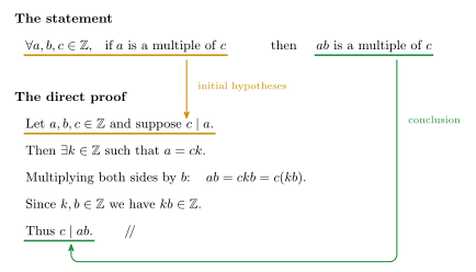
Figure 16: How the statement dictates the first and last lines of a direct proof. One arrow runs from the underlined hypothesis — \(\forall a,b,c \in \mathbb{Z}\), if \(a\) is a multiple of \(c\) — down onto Let \(a,b,c \in \mathbb{Z}\) and suppose \(c \mid a\), and one from the underlined conclusion \(ab\) is a multiple of \(c\) round onto Thus \(c \mid ab\). Both ends of the proof are fixed before any work starts; the three lines between them are the whole content.
Every integer \(n > 1\) is a product of primes
Theorem: every integer \(n > 1\) can be written as a product of primes.
Proof (by contradiction). Suppose the theorem is false. Then there exists an integer \(n > 1\) that is not a product of primes.
Choose the smallest such number \(n\). A smallest such \(n\) exists by the well-ordering principle (see strong-induction-and-the-well-ordering-principle). We choose this \(n\) so that we can use the fact that every integer less than \(n\) (but greater than 1) can be written as a product of primes.
Either \(n\) is prime or \(n\) is composite — splitting into two cases using the fact that every integer \(n > 1\) is one or the other, not both.
Case 1: if \(n\) is prime, then \(n\) is a product of primes — namely the one-term product \(n = p\). Contradiction already.
Case 2: if \(n\) is composite, then \(n = rs\) for some positive integers \(r\) and \(s\) where \(r \neq 1\) and \(s \neq 1\). This implies \(1 < r < n\) and \(1 < s < n\). Because we chose \(n\) to be the smallest integer greater than 1 that is not a product of primes, both \(r\) and \(s\) — which are smaller than \(n\) — must be products of primes: \(r = p_1p_2\cdots p_k\) and \(s = q_1q_2 \cdots q_\ell\). Therefore \[n = rs = p_1 \cdots p_k \, q_1 \cdots q_\ell\] is a product of primes also.
So regardless of whether \(n\) is prime or composite, \(n\) is a product of primes. This contradicts our choice of \(n\), and hence the theorem is proved. \(\square\)
In Case 2, \(r\) and \(s\) must be products of primes precisely because \(n\) was chosen to be the smallest counterexample, so nothing strictly between 1 and \(n\) can be one. The choice of the smallest bad \(n\) is the entire engine of the proof, and it is why the well-ordering principle has to be invoked to make the choice legal.
The proof has three moves. The opening two lines set up the proof by contradiction. The line Choose the smallest such number \(n\) is legal because a smallest such \(n\) exists by the well-ordering principle. Then the proof splits into two cases, using the fact that every integer \(n > 1\) is either prime or composite (not both).
Unique Factorisation Theorem for the integers
Given any integer \(n > 1\), the standard factored form of \(n\) is an expression of the form \[n = p_1^{e_1} p_2^{e_2} \cdots p_k^{e_k}\] where \(k\) is a positive integer, \(p_1, p_2, \dots, p_k\) are prime numbers, \(e_1, e_2, \dots, e_k\) are positive integers, and \(p_1 < p_2 < \cdots < p_k\).
The strict inequality is part of the definition: the primes go in increasing order, which is what makes the form unique rather than merely available.
Worked: 6975 in standard factored form
What is the unique prime factorisation of 6975 in standard factored form? (Q3 of the pre-work questions.)
Try dividing by primes \(2, 3, 5, 7, 11, \dots\), keeping in mind you only have to go as far as \(\sqrt{6975} = 83.51\dots\) because of the lemma below.
\[6975 = 3 \cdot 2325 = 3 \cdot 3 \cdot 775 = 3 \cdot 3 \cdot 5 \cdot 155 = 3 \cdot 3 \cdot 5 \cdot 5 \cdot 31 = 3^2 \cdot 5^2 \cdot 31\]
Counting the divisors. The prime factorisation of a positive divisor of 6975 has 0, 1 or 2 threes; 0, 1 or 2 fives; and 0 or 1 thirty-ones. Thus there are \(3 \cdot 3 \cdot 2 = 18\) positive divisors.
For example, choosing one three, no fives and no thirty-ones gives \(3 = 3^1 \cdot 5^0 \cdot 31^0\), which is indeed a divisor of 6975. Every divisor is one such choice, and different choices give different divisors — which is why the count is a product.
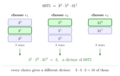
Figure 17: Why 6975 has exactly 18 positive divisors. Picking a divisor of \(3^2 \cdot 5^2 \cdot 31^1\) means picking an exponent from each column independently, so the number of divisors is \(3 \cdot 3 \cdot 2\). The highlighted row in each column is one worked choice — \(e_1 = 1\), \(e_2 = 0\), \(e_3 = 0\) — which yields the divisor 3.
Lemma: for every integer \(n > 1\), if no integer \(x\) in the range \(1 < x \leq \sqrt{n}\) divides \(n\), then \(n\) is prime.
This is what licenses stopping trial division at \(\sqrt{n}\). The proof, by contraposition, is further down.
Worked: the factored form of 1400
(a) Standard factored form of 1400. \[1400 = 2(700) = 2 \cdot 2(350) = 2 \cdot 2(35)(10) = 2^2(5 \cdot 7)(2 \cdot 5) = 2^3 \cdot 5^2 \cdot 7^1\] The final step is where the primes get sorted into increasing order.
(b) \(1400^2\). \[1400^2 = (2^3 \cdot 5^2 \cdot 7^1)^2 = 2^6 \cdot 5^4 \cdot 7^2\] Raising to a power multiplies the exponents.
(c) \(1400^3\). \[1400^3 = (1400)(1400^2) = (2^3 \cdot 5^2 \cdot 7^1)(2^6 \cdot 5^4 \cdot 7^2) = 2^9 \cdot 5^6 \cdot 7^3\] Multiplying adds the exponents, one prime at a time: the \(2\) in \(5^2\) and the \(4\) in \(5^4\) give the \(6\) in \(5^6\).
Both rules are just the index laws, but the standard factored form is what makes them usable: because the form is unique, matching the exponents prime by prime is a legitimate step and not a guess.
(d) How many positive divisors does 1400 have? \[(3+1)(2+1)(1+1) = 4 \cdot 3 \cdot 2 = 24\] Same counting rule as Figure 17, one column per prime: the exponent of 2 can be any of \(0,1,2,3\) (four choices), the exponent of 5 any of \(0,1,2\), the exponent of 7 any of \(0,1\). The \(+1\) in each bracket is the exponent \(0\) — the option of leaving that prime out.
(e) List all positive divisors of 1400 that are divisible by 8.
Since \(8 = 2^3\) and 1400 only carries \(2^3\), “divisible by 8” pins the exponent of 2 at exactly 3. So the answer is all factors of the form \(2^3 \cdot 5^{\ast} \cdot 7^{\ast}\):
| \(7^0\) | \(7^1\) | |
|---|---|---|
| \(5^0\) | 8 | 56 |
| \(5^1\) | 40 | 280 |
| \(5^2\) | 200 | 1400 |
Six of them, which is the counting rule again with one column frozen: \(1 \cdot 3 \cdot 2 = 6\).
(f) Find the smallest positive integer \(n\) such that \(1400n\) is a perfect square.
\(1400n\) is a perfect square if \(\exists t \in \mathbb{Z}\) such that \(1400n = t^2\). Then
\[t^2 = 2^3 \cdot 5^2 \cdot 7^1 \cdot n = \underbrace{(2^2 \cdot 5^1 \cdot 7^1)}_{t} \cdot \underbrace{(2^1 \cdot 5^1 \cdot 7^0 \cdot n)}_{t}\]
The method: try to split each power in half, bigger powers on the left. Both bracketed factors have to equal \(t\), so matching them gives \(2^1 \cdot 5^1 \cdot 7^0 \cdot n = 2^2 \cdot 5^1 \cdot 7^1\), hence
\[n = 2^1 \cdot 7^1 = 14\]
In general: an integer is a perfect square exactly when every exponent in its standard factored form is even, so the smallest useful \(n\) is the product of precisely the primes whose exponent in \(1400\) is odd. Here those are \(2\) (exponent 3) and \(7\) (exponent 1), giving \(n = 2 \cdot 7 = 14\); and \(1400 \cdot 14 = 19600 = 140^2\).
A lemma by contradiction
Lemma: for any integer \(a\) and any prime number \(p\), if \(p \mid a\) then \(p \nmid (a+1)\).
Hint: once the proof is set up, write \((a+1) - a\) in terms of \(p\).
Proof (by contradiction). Let \(a \in \mathbb{Z}\), let \(p\) be prime, and suppose \(p \mid a\) and — for a contradiction — assume \(p \mid (a+1)\). Since \(p \mid a\) there exists \(k \in \mathbb{Z}\) such that \(a = pk\). Since \(p \mid (a+1)\) there exists \(\ell \in \mathbb{Z}\) such that \(a + 1 = p\ell\). So \[1 = (a+1) - a = p\ell - pk = p(\ell - k).\] Since \(\ell, k \in \mathbb{Z}\) we have \(\ell - k \in \mathbb{Z}\). Thus \(1 = p(\ell - k)\) means \(p \mid 1\) — which is a contradiction, because \(p \geq 2\) for every prime, whereas \(p \mid 1\) would force \(p = \pm 1\). So the assumption was false: \(p \nmid (a+1)\).
The technique is to rewrite as equations: the two divisibility statements become the lines \(a = pk\) and \(a+1 = p\ell\). Then combine them so the unwanted quantity is left on its own. Subtracting kills \(a\) and leaves \(1 = p(\ell - k)\), which is the only place the contradiction can come from.
In the same proof, the two existentials get different letters. \(k\) is already spoken for by \(p \mid a\); reusing it for \(p \mid (a+1)\) would assert \(a = a+1\).
In words the lemma says: no prime can divide two consecutive integers. That is exactly what the next theorem needs.
Theorem: there are an infinite number of primes
Proof (by contradiction). Suppose the statement is false — that the number of primes is finite. Then some prime number, say \(p\), is the largest of all the primes, and hence we can list the primes in ascending order: \(2, 3, 5, 7, 11, \dots, p\).
Let \(N\) be 1 more than the product of all the prime numbers, so \(N = (2 \cdot 3 \cdot 5 \cdot 7 \cdot 11 \cdots p) + 1\).
Then \(N > 1\), and so, by the Unique Factorisation Theorem, \(N\) can be written as a product of primes, and hence is divisible by some prime number \(q\). Because \(q\) is prime, it must equal one of the primes in our list \(2, 3, 5, 7, 11, \dots, p\).
Thus, by definition of divisibility, \(q\) divides \(2 \cdot 3 \cdot 5 \cdot 7 \cdot 11 \cdots p\) — that is, \(q \mid (N-1)\) — and so, by the above Lemma, \(q\) does not divide \((2 \cdot 3 \cdot 5 \cdot 7 \cdot 11 \cdots p) + 1 = N\).
Hence \(q\) does divide \(N\) and \(q\) does not divide \(N\), so we have reached a contradiction and we conclude that the original statement must be true. \(\square\)
The pivot is the step \(q \mid (N-1)\), so by the lemma, \(q \nmid N\). The lemma on consecutive integers is the step that closes this proof.
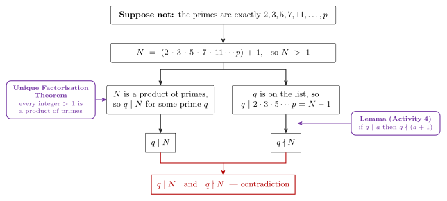
Figure 18: Where each named result plugs into the infinitude-of-primes proof. Two chains start from the same \(N\) and reach opposite verdicts about the same prime \(q\): the left needs the Unique Factorisation Theorem to produce \(q\) at all, the right needs the lemma on consecutive integers to rule it out, and the contradiction is the collision. The right-hand branch is the step \(q \mid (N-1)\), so by the lemma \(q \nmid N\).
The \(\sqrt{n}\) lemma, by contraposition
This closes the loop back to the 6975 factorisation: it is the result that says trial division may stop at \(\sqrt{n}\).
Lemma: for every integer \(n > 1\), if no integer \(x\) in the range \(1 < x \leq \sqrt{n}\) divides \(n\), then \(n\) is prime.
Proof (by contraposition). The contrapositive of the lemma states: \[\forall n \in \mathbb{Z}^{\geq 2}, \text{ if } n \text{ is not prime, then } \exists\, x \in \mathbb{Z} \text{ in the range } 1 < x \leq \sqrt{n} \text{ such that } x \mid n.\]
Suppose \(n \in \mathbb{Z}^{\geq 2}\) and \(n\) is not prime. Then \(n\) is composite so (by definition) \(\exists\, r, s \in \mathbb{Z}^{+}\) such that \(n = rs\) and \(1 < r < n\) and \(1 < s < n\).
Case 1: \(r = s\). In this case, we have \(r = s = \sqrt{n}\).
Case 2: \(r \neq s\). In this case, one of \(r, s\) is less than \(\sqrt{n}\) and the other is greater than \(\sqrt{n}\). (To see why this is, note that if both are greater than \(\sqrt{n}\) we would have \(rs > n\), and if both are less than \(\sqrt{n}\) we would have \(rs < n\).)
In either case, \(\exists\, x \in \{r, s\}\) such that \(1 < x \leq \sqrt{n}\) and \(x\) divides \(n\) (since \(r\) and \(s\) each divide \(n\)). \(\square\)
Two remarks about the scope of the lemma. The proof never finds the factor, it only shows one exists in the range, which is all the lemma claims. And it never rules out a factor above \(\sqrt{n}\): \(194 = 2 \cdot 97\) has \(\sqrt{194} \approx 13.9\), so its factor 97 sits far above the bound while its factor 2 sits below it. The lemma bounds the smallest non-trivial factor, which is exactly what trial division meets first, and that is why the search may stop there.
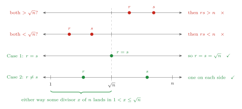
Figure 19: Why a composite \(n = rs\) must have a divisor no larger than \(\sqrt{n}\) — the parenthetical step in the contraposition proof. The two red rows are the possibilities ruled out by size alone: if both are greater than \(\sqrt{n}\) we would have \(rs > n\), and if both are less than \(\sqrt{n}\) we would have \(rs < n\). The two green rows are Case 1 and Case 2 of the proof.
Which proof method, and why
Eight statements are settled above, by four different proof shapes — direct, disproof by counterexample, contradiction and contraposition:
| Statement | Method | Why that one |
|---|---|---|
| \(m \mid (a+b) \to m \mid (a-b)\) | counterexample | one row with hypothesis T and conclusion F kills it |
| \(4 \mid 6m(2m+10m^2)\) | direct | the conclusion is a single divisibility claim, so produce the factor |
| \(a \mid (b+c) \to a \mid b\) or \(a \mid c\) | counterexample | a universal claim is disproved by one bad triple |
| \(c \mid a \to c \mid ab\) | direct | the hypothesis unfolds to \(a = ck\) and the conclusion is one multiplication away |
| every \(n > 1\) is a product of primes | contradiction | needs a smallest offender, which only a contradiction setup provides |
| \(p \mid a \to p \nmid (a+1)\) | contradiction | the conclusion is a non-divisibility, so assume divisibility and break it |
| infinitely many primes | contradiction | a finite list is something you can build \(N\) out of |
| the \(\sqrt{n}\) lemma | contraposition | “no \(x\) divides \(n\)” is an awkward hypothesis; “\(n\) is composite” is a usable one |
The pattern worth carrying: a negative conclusion (\(p \nmid \dots\), “there is no largest prime”) almost always wants contradiction or contraposition, because a negation is hard to build with and easy to break.
See also
- divisibility-and-factorisation · proof-techniques
- strong-induction-and-the-well-ordering-principle — the well-ordering principle the product-of-primes proof leans on
- 2026-08-20-modular-arithmetic — Lecture 11
- practice-problems — §13 Divisibility, with full worked solutions
Lecture 12 — Modular Arithmetic and the Euclidean Algorithm
Pre-work: Video 015 (The Euclidean Algorithm). See gcd-lcm-and-euclidean-algorithm for the reference definitions, worked runs of the algorithm and the gcd/lcm proofs.
Learning goals
- Continue to gain fluency in applying modular arithmetic.
- Understand the definitions of \(\gcd(a,b)\) and \(\operatorname{lcm}(a,b)\) for integers \(a\) and \(b\).
- Be able to apply the Euclidean algorithm to find the greatest common divisor of two integers.
Order, signs and uses
Is \(\gcd(a,b) = \gcd(b,a)\)? Yes.
How do you do gcd and lcm with a mix of positive and negative integers? Take absolute values, as set out below.
Where are gcd, lcm and the Euclidean algorithm used? All the time in arithmetic (adding fractions, etc.); to determine if certain types of equations have solutions; and in cryptography.
Recap on mod
For \(n, d \in \mathbb{Z}\), \(d > 0\): \(n \bmod d = r\) indicates the remainder when \(n\) is divided by \(d\) is \(r\), with \(0 \leq r < d\). For \(m, n, d \in \mathbb{Z}\), \(d > 0\): \(m \equiv n \pmod d\) indicates \(m\) and \(n\) have the same remainder when divided by \(d\) — equivalently \(d \mid (m-n)\). See modular-arithmetic.
Worked: the remainder of \(35m\)
If \(m \in \mathbb{Z}\) and \(m \bmod 6 = 4\), what is the remainder when \(35m\) is divided by 6?
2. Since \(35 \bmod 6 = 5\) and \(m \equiv 4\), we get \(35m \equiv 5 \cdot 4 \equiv 20 \equiv 2 \pmod 6\).
Worked: the remainder of \(3m^2 + 2m + 1\)
If \(m \in \mathbb{Z}\) and \(m \bmod 6 = 4\), what is the remainder when \(3m^2 + 2m + 1\) is divided by 6?
3. \(3m^2 + 2m + 1 \equiv 3(4)^2 + 2(4) + 1 \pmod 6\). Rewrite \(3 \cdot 4^2\) as \(12 \cdot 4\) and the whole term goes — \(12 \bmod 6 = 0\) because \(6 \mid 12\), so \(12(4) \equiv 0 \pmod 6\) — leaving \(8 + 1 = 9 \equiv 3 \pmod 6\).
Rewriting \(3 \cdot 16\) as \(12 \cdot 4\) rather than as \(48\) is the cheaper move: you only need to spot a factor that is \(\equiv 0\), not evaluate the product.
\(\gcd(a,b)\)
Definition: for integers \(a\) and \(b\), not both zero, the greatest common divisor of \(a\) and \(b\), denoted \(\gcd(a,b)\), is the integer \(d\) for which:
- \(d \mid a\) and \(d \mid b\) — \(d\) is a divisor of both \(a\) and \(b\); and
- \(\forall c \in \mathbb{Z}\), if \(c \mid a\) and \(c \mid b\) then \(c \leq d\) — every other divisor of both \(a\) and \(b\) is less than \(d\).
\(\operatorname{hcf}(a,b)\), the highest common factor, names the same object, but \(\gcd\) is the name this course uses. The order of \(a\) and \(b\) does not matter.
What if one, or both, of \(a\) and \(b\) are negative? The divisors of 15 are \(1, 3, 5, 15, -1, -3, -5, -15\) — and these are also the divisors of \(-15\). The divisors of an integer \(a\) are the same as the divisors of \(-a\). Thus \(\gcd(-15, 36) = \gcd(15,36)\), and in general
\[\gcd(a,b) = \gcd(|a|, |b|)\]
\(\gcd(0,b) = b\) for all positive integers \(b\) — this is the base case the algorithm below terminates on.
\(\operatorname{lcm}(a,b)\)
Definition: for non-zero integers \(a\) and \(b\), the lowest (least) common multiple of \(a\) and \(b\), denoted \(\operatorname{lcm}(a,b)\), is the smallest integer \(n\) for which:
- \(n > 0\); and
- \(a \mid n\) and \(b \mid n\) — \(n\) is a multiple of both \(a\) and \(b\).
“Smallest such \(n\)” is doing the work: every other positive multiple of both \(a\) and \(b\) is greater than \(n\).
Order does not matter. The multiples of 5 are \(\dots, -10, -5, 0, 5, 10, 15, \dots\) — the same as the multiples of \(-5\). So \(\operatorname{lcm}(-5, 36) = \operatorname{lcm}(5, 36)\), and in general
\[\operatorname{lcm}(a,b) = \operatorname{lcm}(|a|, |b|)\]
Relationship between gcd and lcm
Use the unique prime factorisation of each integer (see divisibility-and-factorisation). Step 1: write the UPF of each. Step 2: take the minimum exponent of each prime for the gcd and the maximum for the lcm.
\[30 = 2 \cdot 3 \cdot 5 \qquad 72 = 2^3 \cdot 3^2\] \[\gcd(30,72) = 2 \cdot 3 = 6 \qquad \operatorname{lcm}(30,72) = 2^3 \cdot 3^2 \cdot 5 = 360\]
With the two missing exponents written in, \(30 = 2^1 \cdot 3^1 \cdot 5\). The lcm takes the \(5\) of \(30\) and the \(2^3\) and the \(3^2\) of \(72\), giving \(\operatorname{lcm}(30,72) = 2^3 \cdot 3^2 \cdot 5\). The gcd takes the \(2\) and the \(3\), giving \(\gcd(30,72) = 2^1 \cdot 3 = 6\). gcd-lcm-and-euclidean-algorithm lays the same step out as aligned prime columns.
Lemma: if \(a, b \in \mathbb{Z}^+\), then \(\gcd(a,b) \cdot \operatorname{lcm}(a,b) = ab\).
Checking: \(\gcd(30,72) \cdot \operatorname{lcm}(30,72) = 6 \cdot 360 = 30 \cdot 72\), since \((2 \cdot 3)(2^3 \cdot 3^2 \cdot 5) = (2 \cdot 3 \cdot 5)(2^3 \cdot 3^2)\).
More generally, for non-zero integers \(a\) and \(b\): \(\gcd(a,b) \cdot \operatorname{lcm}(a,b) = |ab|\).
Worked: gcd and lcm with a negative argument
\(\gcd(63, -105)\) and \(\operatorname{lcm}(63, -105)\):
- Step 1: \(63 = 3^2 \cdot 7\) and \(-105 = -3 \cdot 5 \cdot 7\). Keep the minus sign out the front and read the primes off the positive part, or replace \(-105\) by \(105\) first.
- Step 2: \(\gcd(63,-105) = 3 \cdot 7 = 21\); \(\operatorname{lcm}(63,-105) = 3^2 \cdot 5 \cdot 7 = 315\).
Either habit gives the same answer, because \(\gcd(a,b) = \gcd(|a|,|b|)\) and \(\operatorname{lcm}(a,b) = \operatorname{lcm}(|a|,|b|)\) — the sign never reaches the answer.
Worked: two distinct primes
Let \(p\) and \(q\) be distinct primes (\(p \neq q\)). Then \(\gcd(p,q) = 1\) and \(\operatorname{lcm}(p,q) = pq\).
The Euclidean algorithm
To determine \(\gcd(a,b)\) for \(a, b \in \mathbb{Z}^+\), based on the fact:
if \(a, b \in \mathbb{Z}\) are not both zero and \(q, r \in \mathbb{Z}\) satisfy \(a = bq + r\), then \(\gcd(a,b) = \gcd(b,r)\).
The proof of this fact is basically showing that every divisor of \(a\) and \(b\) is also a divisor of \(b\) and \(r\), and vice versa:
- Suppose \(c \mid a\) and \(c \mid b\). Then \(c \mid (a - bq)\) and hence \(c \mid r\).
- Suppose \(d \mid b\) and \(d \mid r\). Then \(d \mid (bq + r)\) and hence \(d \mid a\).
Divide the big by the small, then repeat on (small, remainder).
Example: \(\gcd(1232, 5859)\).
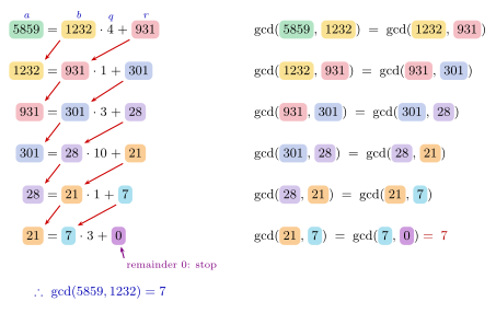
Figure 20: The Euclidean algorithm as a cascade of divisions. Each number is given a capsule colour and keeps it as it migrates: the divisor \(b\) of one line becomes the dividend \(a\) of the next, and the remainder \(r\) becomes the next divisor — the two red arrows per step. The right-hand column is the same movement written as \(\gcd(a,b) = \gcd(b,r)\), so the pair shrinks without the gcd ever changing, until the remainder hits 0 and \(\gcd(7,0) = 7\) can be read off.
Therefore \(\gcd(5859, 1232) = 7\). In \(\gcd(1232, 5859)\), label \(1232\) as \(b\) and \(5859\) as \(a\) before starting, so that the first division is big-by-small.
Worked: \(\gcd(4131, 2431)\)
Use the Euclidean Algorithm to determine \(\gcd(4131, 2431)\).
| \(a\) | \(=\) | \(b \times q\) | \(+ \; r\) |
|---|---|---|---|
| 4131 | \(=\) | \(2431 \times 1\) | \(+ \; 1700\) |
| 2431 | \(=\) | \(1700 \times 1\) | \(+ \; 731\) |
| 1700 | \(=\) | \(731 \times 2\) | \(+ \; 238\) |
| 731 | \(=\) | \(238 \times 3\) | \(+ \; 17\) |
| 238 | \(=\) | \(17 \times 14\) | \(+ \; 0\) |
\[\gcd(4131, 2431) = \cdots = \gcd(238, 17) = \gcd(17, 0) = \mathbf{17}\]
An “if and only if” proof
Prove that for all positive integers \(a\) and \(b\), \(a \mid b\) if and only if \(\operatorname{lcm}(a,b) = b\).
This calls for a direct proof, not a counterexample: the claim is universally quantified and true, so there is nothing to disprove. Both halves of the definition of lcm get used — \(n > 0\), and \(a \mid n\) and \(b \mid n\) — and so does the word smallest in it.
Method 1: prove each direction separately. This is the recommended method.
The forward direction:
(\(\Rightarrow\)) Suppose \(a, b \in \mathbb{Z}^+\) and suppose \(a \mid b\). Then \(\exists k \in \mathbb{Z}\) such that \(b = ka\). So \(\operatorname{lcm}(a,b) = \operatorname{lcm}(a, ka)\). Since \(a \mid ka\) and \(ka \mid ka\) and no smaller \(n > 0\) has \(ka \mid n\), \(\therefore \operatorname{lcm}(a, ka) = ka\) — and \(b = ka\) — \(\therefore \operatorname{lcm}(a,b) = b\).
The reverse direction, as a skeleton:
(\(\Leftarrow\)) Suppose \(a, b \in \mathbb{Z}^+\) and suppose \(\operatorname{lcm}(a,b) = b\). \(\vdots\) (prove) \(\therefore a \mid b\).
Filling the gap: by the definition of \(\operatorname{lcm}\), \(a \mid \operatorname{lcm}(a,b)\). Substituting the hypothesis \(\operatorname{lcm}(a,b) = b\) gives \(a \mid b\) at once. \(\square\)
On the forward direction: the clause “no smaller \(n > 0\) has \(ka \mid n\)” is where the word least in least common multiple is discharged. It holds because any positive \(n\) divisible by \(ka\) satisfies \(n \geq ka\).
Method 2: prove both directions simultaneously. Be careful: this is the quicker method, but it is easy to make a logical error.
This rewrites the same lines, replacing each connective with an “iff”: “Then”, “So” and “Since” become “This is true iff”, “which holds iff” and “this holds iff”, five links in all:
Suppose \(a, b \in \mathbb{Z}^+\) and suppose \(a \mid b\).
— This is true iff \(\exists k \in \mathbb{Z}\) such that \(b = ka\), — which holds iff \(\operatorname{lcm}(a,b) = \operatorname{lcm}(a, ka)\), — this holds iff \(a \mid ka\) and \(ka \mid ka\) and no smaller \(n > 0\) has \(ka \mid n\), — which holds iff \(\operatorname{lcm}(a, ka) = ka\) — and \(b = ka\) — — which holds iff \(\operatorname{lcm}(a,b) = b\).
One pass instead of two, at the price that every link must genuinely be reversible. That is the logical error to watch for: if any single line is only an implication, the chain quietly proves one direction and reads as though it proved both.
The same statement, and a second gcd/lcm biconditional, are also written out in gcd-lcm-and-euclidean-algorithm.
Challenge: reversing the Euclidean algorithm
Non-assessed content.
Theorem: for \(a, b, c \in \mathbb{Z}\), if \(\gcd(a,b) \mid c\) then there exist integers \(x\) and \(y\) such that \(ax + by = c\).
Given \(ax + by = c\), use the Euclidean algorithm to find \(\gcd(a,b)\), then run the steps in reverse to find \(x\) and \(y\).
Example: find integers \(x, y\) satisfying \(1232x + 5859y = 14\).
Step 1 — use the E.A. to find \(\gcd(1232, 5859) = 7\):
\[5859 = 1232 \cdot 4 + 931 \quad \text{(Eqn 1)}\] \[1232 = 931 \cdot 1 + 301 \quad \text{(Eqn 2)}\] \[931 = 301 \cdot 3 + 28 \quad \text{(Eqn 3)}\] \[301 = 28 \cdot 10 + 21 \quad \text{(Eqn 4)}\] \[28 = 21 \cdot 1 + 7 \quad \text{(Eqn 5)}\] \[21 = 7 \cdot 3 + 0\]
Step 2 — work backwards to get \(1232w + 5859z = 7\):
From Eqn 5: \(7 = 28 - 21\). Use Eqn 4 to replace the 21 and collect like terms: \(7 = 28 - (301 - 28 \cdot 10) = 28 \cdot 11 - 301\). Use Eqn 3 to replace the 28: \(7 = (931 - 301 \cdot 3)\cdot 11 - 301 = 931 \cdot 11 - 301 \cdot 34\). Use Eqn 2 to replace the 301: \(7 = 931 \cdot 11 - (1232 - 931)\cdot 34 = 931 \cdot 45 - 1232 \cdot 34\). Use Eqn 1 to replace the 931: \(7 = (5859 - 1232 \cdot 4)\cdot 45 - 1232 \cdot 34 = 5859 \cdot 45 - 1232 \cdot 214\).
Step 3 — multiply through to get \(1232x + 5859y = 14\):
Therefore \(7 = 1232(-214) + 5859(45)\), so \(14 = 1232(-428) + 5859(90)\).
See also
- gcd-lcm-and-euclidean-algorithm · modular-arithmetic · divisibility-and-factorisation
- 2026-08-20-modular-arithmetic — Lecture 11
- practice-problems — §15 The Euclidean Algorithm, with full worked solutions
Lecture 11 — Modular Arithmetic
Pre-work: Video 014 (Modular Arithmetic). See modular-arithmetic for the reference definitions, the quotient-remainder theorem and the congruence lemma this lecture builds on.
Learning goals
- Understand the proof that there are an infinite number of primes. (See 2026-08-17-divisibility.)
- Understand the definition of floor and ceiling.
- Understand the quotient-remainder theorem.
- Gain fluency in applying modular arithmetic.
Common questions
How does the quotient-remainder theorem work with negative integers? The remainder is still required to satisfy \(0 \leq r < d\), so it stays non-negative: \(-19 = 6 \cdot (-4) + 5\), giving \(-19 \bmod 6 = 5\).
What is the difference between using mod with an equal sign and with an equivalence sign? See “Take care with notation” below, and “\(\bmod\) versus \(\equiv\)” in modular-arithmetic — this is the notational trap of the topic.
Floor and ceiling
For the floor you move left on the number line, so \(\lfloor -3.2 \rfloor = -4\). For the ceiling you move right, so \(\lceil -3.2 \rceil = -3\). (And \(\lfloor 3.2 \rfloor = 3\), \(\lceil 3.2 \rceil = 4\).) Watch out for the negatives.
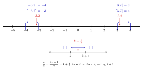
Figure 21: Floor and ceiling on the number line. Floor hops left to the nearest integer, ceiling hops right; it is that direction — not the differing arrow lengths — that the negative case gets wrong, giving \(\lfloor -3.2 \rfloor = -4\) rather than \(-3\). The lower line is the proof trick: for odd \(n\), \(n/2\) lands strictly between the integers \(k\) and \(k+1\), so the floor and ceiling can be read straight off.
The awkward case can be rewritten as an integer plus a bit: \(-3.2 = -4 + 0.8\), so \(\lfloor -3.2 \rfloor = \lfloor -4 + 0.8 \rfloor = -4\) with no thinking required. That is the same manoeuvre as the \(k + \frac{1}{2}\) line in Figure 21, and it is the one to reach for in a proof.
To use floor or ceiling in a proof, it is often helpful to write an expression as an integer plus an amount between 0 and 1. For example, to prove that “if \(n\) is an odd integer, then \(\lceil \frac{n}{2}\rceil = \lfloor \frac{n}{2} \rfloor + 1\)”, write
\[\frac{n}{2} = \frac{2k+1}{2} = k + \frac{1}{2}\]
for some integer \(k\) — and \(k + \frac{1}{2}\) sits between \(k\) and \(k+1\), so the floor is \(k\) and the ceiling is \(k+1\). The same trick handles \(\big\lfloor (p^3 + 4p^2 + 5) + \frac{1}{4} \big\rfloor\) where \(p \in \mathbb{Z}\).
Quotient-remainder theorem and “mod”
Given any integer \(n\) and positive integer \(d\), there exist unique integers \(q\) and \(r\) such that \(n = dq + r\) and \(0 \leq r < d\).
The quotient is \(q = \lfloor \frac{n}{d} \rfloor\) and the remainder is \(r = n - d\lfloor \frac{n}{d} \rfloor\). We define \(n \bmod d = r\).
With \(d = 6\): \(53 = 6 \cdot 8 + 5\), \(20 = 6 \cdot 3 + 2\), \(-19 = 6 \cdot (-4) + 5\).
This is primary-school long division: \(3\,\overline{)\,122}\) giving \(40\) remainder \(2\) is the same statement as \(122 = 3 \cdot 40 + 2\), and in general \(d\,\overline{)\,n}\) gives \(q\) remainder \(r\). The one thing school long division does not tell you is what happens when \(n\) is negative, which is what the \(0 \leq r < d\) clause settles. See modular-arithmetic for that case drawn on the number line.
Two equivalent ways of defining \(m \equiv n \pmod d\)
- Definition 1: \(m\) and \(n\) are congruent modulo \(d\) iff they have the same remainder according to the quotient-remainder theorem.
- Definition 2: \(m \equiv n \pmod d\) iff \(d \mid (m-n)\).
In the examples above, 53 and \(-19\) are congruent modulo 6: \(53 \equiv -19 \pmod 6\). Checking with Definition 2: does \(6 \mid \big(53 - (-19)\big)\)? We have \(53 + 19 = 72\) and \(6 \mid 72\), so yes.
However 53 and 20 have different remainders on division by 6, so \(53 \not\equiv 20 \pmod 6\).
Take care with notation
- For \(n, d \in \mathbb{Z}\), \(d > 0\): \(n \bmod d = r\) indicates that the remainder when \(n\) is divided by \(d\) is \(r\), with \(0 \leq r < d\).
- For \(m, n, d \in \mathbb{Z}\), \(d > 0\): \(m \equiv n \pmod d\) indicates that \(m\) and \(n\) have the same remainder when divided by \(d\) — equivalently \(d \mid (m-n)\).
E.g. \(5 \bmod 4 = 1\) and \(9 \bmod 4 = 1\), so \(9 \equiv 5 \pmod 4\) — but \(9 \bmod 4 \neq 5\).
Q4 from the pre-class multiple choice questions
True or false? \(-50 \equiv 22 \pmod 8\). True, both ways:
- Definition 1: \(-50 = -48 - 2 = -56 + 6 = 8(-7) + 6\), so \(-50 \bmod 8 = 6\); and \(22 = 16 + 6\), so \(22 \bmod 8 = 6\). Same remainder.
- Definition 2: \(22 - (-50) = 72 = 8 \times 9\), so \(8 \mid \big(22-(-50)\big)\).
Worked: \(-32\) divided by \(5\)
- \(\left\lfloor \frac{-32}{5} \right\rfloor\) and \(\left\lceil \frac{-32}{5} \right\rceil\):
- Fraction approach: \(\lfloor \frac{-30}{5} - \frac{2}{5} \rfloor = \lfloor -6 - \frac{2}{5} \rfloor = -7\) (smaller than \(-6\)).
- Decimal approach: \(\lfloor -6.4 \rfloor = \lfloor -6 - 0.4 \rfloor = -7\).
So \(\left\lfloor \frac{-32}{5} \right\rfloor = -7\) and \(\left\lceil \frac{-32}{5} \right\rceil = -6\).
\(\lceil x \rceil = \lfloor x \rfloor + 1\) only when \(x\) is not an integer; when \(x \in \mathbb{Z}\) the two are equal. That’s exactly why the result \(\lceil n/2 \rceil = \lfloor n/2 \rfloor + 1\) is stated only for odd \(n\).
Quotient and remainder for \(n = -32\), \(d = 5\): \(-32 = -7 \cdot 5 + 3\), so \(q = -7\) and \(r = 3\).
\(-32 \bmod 5 = 3\).
Is \(-32 \equiv 32 \pmod 5\)? By Definition 2: \(32 - (-32) = 64\), and \(5 \nmid 64\), so no — \(32 \not\equiv -32 \pmod 5\).
Integers between 10 and 20 congruent to \(-32\) modulo 5: those leaving remainder 3, i.e. 13 and 18.
On a number line: mark 10 (which is \(\equiv 0\), since \(5 \mid 10\)), count 3 to the right to reach the first member 13, then hop \(+5\) to 18 and \(+5\) again to 23 — which has overshot 20, so the hunt stops. A congruence class is an arithmetic progression of step \(d\), and finding its members inside a range is just walking it.
Worked: \(n^2 \bmod 4\) for odd \(n\)
(a) Prove that for any odd integer \(n\), \(n^2 \bmod 4 = 1\).
Direct proof. Suppose \(n\) is odd. Then \(\exists k \in \mathbb{Z}\) such that \(n = 2k+1\). So \[n^2 = (2k+1)^2 = 4k^2 + 4k + 1 = 4(k^2 + k) + 1.\] Since \(k^2 + k \in \mathbb{Z}\), this gives by the QR theorem: \(n^2 \bmod 4 = 1\). \(\square\)
What licenses reading the remainder straight off that last line is the theorem’s uniqueness clause together with the range check \(0 \leq r < d\) — here \(0 \leq 1 < 4\). Without the range check, \(n^2 = 4(k^2+k-1) + 5\) would be an equally valid rearrangement.
Four marks are accepted for “end of proof” in this course: //, \(\square\), \(\blacksquare\), or QED.
(b) Use this fact to show that for any odd integer \(n\), \(\left\lfloor \frac{n^2}{4} \right\rfloor = \frac{n^2 - 1}{4}\).
Method 1 — show LHS \(=\) RHS using \(n = 2k+1\):
\[\text{LHS} = \left\lfloor \frac{(2k+1)^2}{4} \right\rfloor = \left\lfloor \frac{4k^2+4k+1}{4} \right\rfloor = \left\lfloor (k^2+k) + \frac{1}{4} \right\rfloor = k^2 + k\] \[\text{RHS} = \frac{(2k+1)^2 - 1}{4} = \frac{4k^2+4k+1-1}{4} = k^2 + k\]
so LHS \(=\) RHS.
Method 2 — use the rule \(r = n - d\lfloor \frac{n}{d} \rfloor\) with number \(n^2\), divisor 4, remainder 1:
\[1 = n^2 - 4\left\lfloor \frac{n^2}{4} \right\rfloor \implies 4\left\lfloor \frac{n^2}{4} \right\rfloor = n^2 - 1 \implies \left\lfloor \frac{n^2}{4}\right\rfloor = \frac{n^2-1}{4}\]
Modular arithmetic — the congruence lemma
Lemma: if \(a \equiv b \pmod d\) and \(m \equiv n \pmod d\), then \[a + m \equiv b + n \pmod d \qquad \text{and} \qquad am \equiv bn \pmod d\]
For example, \(8 \equiv 2 \pmod 3\) and \(46 \equiv 1 \pmod 3\), so \(8 \cdot 46 \equiv 2 \cdot 1 \equiv 2 \pmod 3\), and \(8 + 46 \equiv 2 + 1 \equiv 0 \pmod 3\).
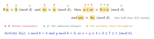
Figure 22: How the lemma is actually used: the numbers of the worked example below sit directly above the lemma’s slots. Reading down a column tells you what to substitute — the known remainders 4 and 3 go into the \(a\) and \(m\) slots, the unknown integers \(x\) and \(y\) into \(b\) and \(n\), and the modulus 6 is the same in every slot. The multiplication half is stated with nothing substituted.
Worked: sums and products mod 6
Suppose \(x \bmod 6 = 4\) and \(y \bmod 6 = 3\).
(a) \((x+y) \bmod 6\): \[x + y \equiv 4 + 3 \equiv 7 \equiv 1 \pmod 6\] so the answer is 1.
(b) \((5x^2 + 4y) \bmod 6\): \[5x^2 + 4y \equiv 5(4)^2 + 4(3) \equiv 5(16) + 12 \equiv 5(16) \equiv 5(4) \equiv 20 \equiv 2 \pmod 6\] The lemma licenses each step: the first substitution, then its \(+\) half for dropping the \(12\) (since \(12 \equiv 0 \pmod 6\)), and its \(\times\) half for replacing \(16\) by \(4\). The answer is 2.
Reducing at every step is what keeps the numbers small.
Remainders and divisibility tests
Modular arithmetic explains the common divisibility tests.
A positive integer is divisible by 3 if and only if the sum of its digits is divisible by 3.
Example: 254 is not divisible by 3 — the sum of its digits is \(2+5+4 = 11\), not divisible by 3.
\[254 \equiv 2 \cdot 100 + 5 \cdot 10 + 4 \cdot 1 \equiv 2 \cdot 1 + 5 \cdot 1 + 4 \cdot 1 \equiv 2 + 5 + 4 \equiv 11 \equiv 2 \pmod 3\]
so the remainder is 2 (confirming with the quotient-remainder theorem: \(254 = 3 \cdot 84 + 2\)).
Example: 3252 is divisible by 3, because \(3+2+5+2 = 12\) is.
\[3252 \equiv 3 \cdot 1 + 2 \cdot 1 + 5 \cdot 1 + 2 \cdot 1 \equiv 12 \equiv 0 \pmod 3 \implies 3 \mid 3252\]
The test works because \(\forall a \in \mathbb{Z}^+\), \(10^a \equiv 1 \pmod 3\). To see \(10^2 \equiv 1 \pmod 3\), use the lemma with \(a = m = 10\) and \(b = n = 1\); to see \(10^3 \equiv 1 \pmod 3\), use the lemma with \(a = 10^2\), \(m = 10\), \(b = n = 1\); and so on.
See also
- modular-arithmetic · divisibility-and-factorisation
- 2026-08-20-euclidean-algorithm — Lecture 12
- practice-problems — §14 Modular Arithmetic, with full worked solutions
Week 5
Lecture 13 — Sequences and Mathematical Induction
Pre-work: Video 016 (Sequences) and Video 017 (Mathematical Induction). See sequences-and-summations for the notation and sum manipulations, and mathematical-induction for the proof template, the worked examples and the inequality rules. The worked questions are below.
Learning goals
- Gain fluency in the use of standard notation for sequences and summations.
- Understand how to apply the principle of mathematical induction to prove properties of summations and inequalities.
The first goal is about four notations: \((a_n)_{n \geq 0}\), \(\{a_n\}_{n=1}^{\infty}\), \(a_1, a_2, a_3, \dots\) and \(\sum_{n=1}^{m} a_n\).
Two questions about induction proofs
Do we have to write/know basis step, inductive hypothesis etc? It is a good idea to list these explicitly in your proofs to help the reader to follow the proof.
How does the LHS = RHS in the example from video 17? \(P(k)\) is the statement \(1 + 2 + \cdots + k = \frac{k(k+1)}{2}\), so \(P(k+1)\) is the statement \(1 + 2 + \cdots + k + (k+1) = \frac{(k+1)(k+2)}{2}\). Working from the left:
\[L.H.S = \underbrace{1 + 2 + \cdots + k}_{\text{arithmetic series}} + (k+1) = \frac{k(k+1)}{2} + (k+1) = \frac{k(k+1)}{2} + \frac{2(k+1)}{2} = \frac{(k+1)(k+2)}{2} = R.H.S\]
The step that does the work is replacing \(1 + 2 + \cdots + k\) — an arithmetic series — by the closed form the inductive hypothesis supplies.
Defining a sequence
Three ways: by an explicit formula, recursively from one or more preceding terms, or in words. Full definitions and examples in sequences-and-summations.
Sequences cannot be defined by listing their first few terms (unless you can list all of them). Asked for the next term after \(1, 4, 9, 16\): under \(a_n = n^2\) it is 25; under \(a_n = n^2 \bmod 20\) it is 5. Searching the Online Encyclopedia of Integer Sequences (https://oeis.org) for \(1, 4, 9, 16\) returns 397 possible sequences.
Working with sums
\[\sum_{i=m}^{n} a_i \pm \sum_{i=m}^{n} b_i = \sum_{i=m}^{n}(a_i \pm b_i) \qquad\qquad \sum_{i=m}^{n} c\,a_i = c\sum_{i=m}^{n} a_i\]
Worked: change of variable
(a) What expression results from applying the change of variable \(j = i+1\) to \(\displaystyle\sum_{i=0}^{n-1}(2i+5)\)?
With \(i = j - 1\):
- lower limit: \(j = 0 + 1 = 1\)
- upper limit: \(j = (n-1) + 1 = n\)
- general term: \(2i + 5 = 2(j-1) + 5 = 2j + 3\)
\[\sum_{i=0}^{n-1}(2i+5) = \sum_{j=1}^{n}(2j+3)\]
(b) Use the change of variable from part (a) to simplify \(\displaystyle 3\sum_{j=1}^{n}(j^2+2j) + \sum_{i=0}^{n-1}(2i+5)\).
Rewriting the second sum over \(j\) puts both sums on the same index range, so they can be combined termwise:
\[\sum_{j=1}^{n} 3(j^2+2j) + \sum_{j=1}^{n}(2j+3) = \sum_{j=1}^{n}\Big(3(j^2+2j) + (2j+3)\Big) = \sum_{j=1}^{n}\big(3j^2 + 8j + 3\big)\]
Q4 from the pre-class multiple choice questions
The point of the question is splitting off the last term of a sum, which is done often when proving a summation property by mathematical induction:
\[\sum_{i=1}^{n+1}(3i+2) = \underbrace{(3\cdot1+2)}_{i=1} + \underbrace{(3\cdot2+2)}_{i=2} + \cdots + \underbrace{(3n+2)}_{i=n} + \underbrace{(3(n+1)+2)}_{i=n+1} = \sum_{i=1}^{n}(3i+2) + \big(3(n+1)+2\big)\]
Worked: three rewrites of one sum
Let \(k \in \mathbb{Z}\), \(k \geq 2\). Which of the following expressions is equal to \(\displaystyle\sum_{i=1}^{k+1}(2i-1)\)?
The restriction \(k \geq 2\) matters for option C: \(\sum_{i=1}^{k-1}(2i-1) + 4k\) only has something to sum once \(k - 1 \geq 1\).
All three of A, B and C. Each is the same sum described differently:
- A. \(\displaystyle\sum_{j=0}^{k}(2j+1)\) — a change of variable, \(j = i - 1\). The limits shift from \(1 \dots k+1\) to \(0 \dots k\), and \(2i - 1 = 2(j+1) - 1 = 2j + 1\).
- B. \(\displaystyle\sum_{i=1}^{k}(2i-1) + 2k + 1\) — split off the last term, \(i = k+1\), which is \(2(k+1) - 1 = 2k + 2 - 1 = 2k+1\).
- C. \(\displaystyle\sum_{i=1}^{k-1}(2i-1) + 4k\) — split off the last two terms, \(i = k\) and \(i = k+1\), which together give \((2k-1) + (2k+1) = 4k\).
Written as sigma notation the three look like different objects. Written out as terms they are visibly one list, bracketed three ways (Figure 23). The split in B is the one worth memorising: it is the move Q4 is about — splitting off the last term — and the move every induction proof over a sum begins with.
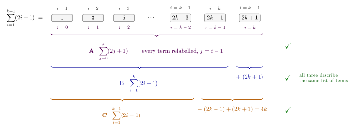
Figure 23: One sum, three groupings — why all three options are correct. The boxed row is \(\sum_{i=1}^{k+1}(2i-1)\) written out. A keeps every term and only relabels the index (\(j = i-1\)); B brackets off the last term; C brackets off the last two and adds them, \((2k-1)+(2k+1) = 4k\). Nothing is added or removed in any of the three.
Mathematical induction
Let \(P(n)\) be a predicate in some integer \(n\). Given that (1) \(P(2)\) is true and (2) \(\forall k \in \mathbb{Z}\) with \(k \geq 2\), if \(P(k)\) then \(P(k+1)\) — then \(P(5)\) follows by applying (2) three times, and in fact \(P(n)\) is true for each integer \(n \geq 2\). The chain of modus ponens steps, and why the basis step is not optional, are in mathematical-induction.
The worked summation example — \(\displaystyle\sum_{i=1}^{n}(3i+2) = \frac{3n^2+7n}{2}\) for each integer \(n \geq 1\) — is written out there in full, with the four steps every induction proof takes: 1 define the predicate, 2 base case, 3 assume the inductive hypothesis \(P(k)\), 4 prove \(P(k+1)\).
Worked: a summation proof
Prove that for each integer \(n \geq 1\), \(\displaystyle\sum_{i=1}^{n}(2i-1) = n^2\).
Let \(P(n)\) be the predicate \(\displaystyle\sum_{i=1}^{n}(2i-1) = n^2\).
Basis step (\(n = 1\)). LHS of \(P(1)\): \(\displaystyle\sum_{i=1}^{1}(2i-1) = 2 - 1 = 1\). RHS of \(P(1)\): \(1^2 = 1\). Therefore \(P(1)\) is true.
Inductive step. Prove \(P(k) \to P(k+1)\) for all \(k \geq 1\) where \(k \in \mathbb{Z}\).
Suppose \(P(k)\) holds. Then \(\displaystyle\sum_{i=1}^{k}(2i-1) = k^2\).
LHS of \(P(k+1)\):
\[\sum_{i=1}^{k+1}(2i-1) = \sum_{i=1}^{k}(2i-1) + \big(2(k+1)-1\big) = k^2 + 2k + 1 \qquad \text{(by the inductive hypothesis } P(k)\text{)}\] \[= (k+1)^2\]
which is the RHS of \(P(k+1)\). Therefore \(P(k) \to P(k+1)\). //
Conclusion. Therefore, by the principle of mathematical induction, \(\displaystyle\sum_{i=1}^{n}(2i-1) = n^2\) for each integer \(n \geq 1\).
The // marks the end of the inductive step. The concluding sentence finishes the proof.
Mathematical induction to prove an inequality
You must be careful when manipulating inequalities — the full table of what can and cannot be concluded is in mathematical-induction. The two traps: multiplying by a negative flips the direction, and \(a < b\) together with \(x > y\) lets you conclude nothing about \(a + x\).
The example from the second video, \(n^2 < 2^n\) for each integer \(n \geq 5\), is worked through there as well.
Worked: an inequality proof
Prove that for each integer \(n \geq 2\), \(5^n + 9 < 6^n\).
Let \(P(n)\) be the predicate \(5^n + 9 < 6^n\).
Basis step (\(n = 2\)). LHS of \(P(2) = 5^2 + 9 = 25 + 9 = 34\); RHS of \(P(2) = 6^2 = 36\). Since \(34 < 36\), \(P(2)\) is true.
Inductive step. Prove \(P(k) \to P(k+1)\) for all \(k \geq 2\), \(k \in \mathbb{Z}\).
Assume \(P(k)\): \(5^k + 9 < 6^k\). The goal is \(P(k+1)\): \(5^{k+1} + 9 < 6^{k+1}\).
\[\text{LHS of } P(k+1) = 5^{k+1} + 9 = 5(5^k + 9) - 4 \times 9\] \[< 5(6^k) - 4 \times 9 \qquad \text{(by the inductive hypothesis } P(k)\text{)}\] \[< 6 \cdot 6^k - 4 \times 9 \qquad (5 < 6)\] \[< 6^{k+1} \qquad (-4 \times 9 < 0)\]
which is the RHS of \(P(k+1)\). Therefore \(P(k) \to P(k+1)\). //
Conclusion. Therefore, by the principle of mathematical induction, \(5^n + 9 < 6^n\) for each integer \(n \geq 2\).
The opening rewrite is the trick worth remembering: \(5(5^k + 9) - 4 \times 9 = 5^{k+1} + 45 - 36 = 5^{k+1} + 9\), which manufactures the exact expression \(5^k + 9\) that the inductive hypothesis bounds.
See also
- sequences-and-summations · mathematical-induction · proof-techniques
- 2026-08-20-euclidean-algorithm — Lecture 12
- practice-problems — §16 Sequences, with full worked solutions
- practice-problems — §17 Mathematical Induction, with full worked solutions
Lecture 14 — Strong Mathematical Induction and the Well-Ordering Principle
Pre-work: Video 018 (Strong Mathematical Induction and the Well-Ordering Principle). See strong-induction-and-the-well-ordering-principle for the principles themselves, the MI/SMI comparison and the worked examples; the questions worked below apply them. mathematical-induction has the ordinary-induction template both methods share.
Learning goals
- Gain fluency in applying the principles of mathematical induction and strong mathematical induction.
- Further your understanding of how the basis step relates to the inductive step in mathematical induction and strong mathematical induction.
- Appreciate the equivalence between mathematical induction, strong mathematical induction and the well-ordering principle for the integers.
Base cases, least elements and equivalence
Why does pre-class Q1 need 2 values for the basis step, not 3? Because the recurrence in that question, \(b_n = b_{n-2} + b_{n-1}\), reaches back exactly two terms — so the inductive step consumes \(P(k-1)\) and \(P(k)\), and the basis step has to cover \(P(1)\) and \(P(2)\) for the chain to have somewhere to start. Worked in full below. Contrast the sequence \(a_n = a_{n-1} - a_{n-3}\) further down, whose recurrence reaches back three terms and therefore needs three base cases.
In the well-ordering principle — non-empty set, fixed integer, a least element — is the least element an integer in the set or one outside it? In the set — a least element of \(S\) is a member of \(S\) that is \(\leq\) every member of \(S\), not a bound sitting outside it. (A lower bound is allowed to sit outside: the “fixed integer” in the statement is any integer below everything in \(S\), and it need not belong to \(S\) — \(-1\) plays that role for the set of squares below. The two ideas are easy to run together, and the difference is the whole content of the principle: bounds are cheap, a least element is what the WOP promises.) The terminology is unpacked in strong-induction-and-the-well-ordering-principle; four sets are tested against the principle below and drawn together in one figure.
Why are mathematical induction, strong mathematical induction and the well-ordering principle for the integers all equivalent? Anything provable by one is provable by the other two — SMI becomes MI by rewording the predicate to accumulate every earlier case (Epp Q27 p. 279), and MI becomes the WOP by contradiction on the set of counterexamples (Epp Q31 p. 279). One example is proved all three ways; see the same note.
Mathematical induction vs strong mathematical induction
The two differ only in what the inductive step may assume, and correspondingly in how much the basis step must establish. Given the basis \(P(2) \wedge P(3) \wedge P(4)\) and the SMI inductive step \(\forall k \geq 4\), \(\big(P(2) \wedge \cdots \wedge P(k)\big) \to P(k+1)\), we reach \(P(6)\) in two applications — and in fact \(P(n)\) for each integer \(n \geq 2\), exactly as ordinary induction does from \(P(2)\) alone. Side-by-side in strong-induction-and-the-well-ordering-principle.
Worked: \(4 \mid b_n\) (pre-class Q1)
Suppose \(b_1, b_2, b_3, \dots\) is defined by \(b_1 = 4\), \(b_2 = 12\), and \(b_n = b_{n-2} + b_{n-1}\) for each integer \(n \geq 3\). Prove that \(4 \mid b_n\) for each integer \(n \geq 1\).
The recurrence reaches back two terms, so this needs two base cases. The proof is by PSMI. The first few terms:
\[b_3 = b_1 + b_2 = 4 + 12 = 16 \qquad b_4 = b_2 + b_3 = 12 + 16 = 28\]
The full proof by strong induction is in strong-induction-and-the-well-ordering-principle. The point of the example: the inductive step uses both \(P(k)\) and \(P(k-1)\), which is exactly what ordinary induction cannot supply.
Worked: a recurrence that reaches back three terms
Suppose \(a_0, a_1, a_2, \dots\) is defined by \(a_0 = 6\), \(a_1 = 9\), \(a_2 = 12\) and \(a_n = a_{n-1} - a_{n-3}\) for each integer \(n \geq 3\).
(a) Determine the value of \(a_4\).
\(a_4\) cannot be reached in one step, because the recurrence at \(n = 4\) asks for \(a_3\), which has not been computed yet. Two steps:
\[a_3 = a_2 - a_0 = 12 - 6 = 6 \qquad a_4 = a_3 - a_1 = 6 - 9 = -3\]
The sequence is not monotone and not positive — \(6, 9, 12, 6, -3, \dots\) — so nothing about “divisible by 3” can be read off a pattern of growth. It has to be proved.
(b) In a proof by strong mathematical induction that \(3 \mid a_n\) for each integer \(n \geq 0\), what would you need to prove in the basis step?
With \(P(n)\) the predicate \(3 \mid a_n\), the recurrence reaches back three terms, so the basis step needs three cases:
\[P(0):\; 3 \mid a_0 \qquad P(1):\; 3 \mid a_1 \qquad P(2):\; 3 \mid a_2\]
The count is read straight off the recurrence: the term \(a_{n-3}\) means 3 cases. It is the deepest back-reference that sets the number, not the number of terms on the right-hand side — strong-induction-and-the-well-ordering-principle has a figure contrasting this recurrence with the one for \(b_n\) above.
This is the sequence used below to compare three separate proofs of \(3 \mid a_n\) — by SMI, by MI, and by the WOP.
Every integer \(n > 1\) is a product of primes
Proved by strong induction, splitting on whether \(k+1\) is prime or composite; written out in strong-induction-and-the-well-ordering-principle. Strong induction is required rather than ordinary induction because \(r\) and \(s\) in the factorisation \(k+1 = rs\) can be any integers from 2 to \(k\) — the proof has no control over which, so it needs the inductive hypothesis at all of those values.
The prose proof leaves the induction machinery implicit. It is worth writing each part out in terms of a predicate:
| Part of the proof | In terms of \(P\) |
|---|---|
| the theorem | \(P(n)\): \(n\) can be written as a product of primes, for \(n \geq 2\) (the same as \(n > 1\)) |
| the basis step | \(P(2)\) ✓ |
| the inductive step | \(\big(P(2) \wedge P(3) \wedge \cdots \wedge P(k)\big) \to P(k+1)\) |
| “\(1 < r < k+1\) and \(1 < s < k+1\)” | \(P(r) \wedge P(s)\), both taken from the conjunction above |
| “In either case…” | \(P(2) \wedge \cdots \wedge P(k) \to P(k+1)\) again, closing the step |
Naming the predicate first, then writing out the exact implication the inductive step owes you, is what turns the prose proof into the course’s induction skeleton.
The well-ordering principle for the integers
Let \(S\) be a non-empty set of integers, each of which is greater than some fixed integer. Then \(S\) has a least element.
Three conditions. The four sets below test them — one per condition, plus one case where they all hold. The one that is easiest to forget is “of integers”: a set can be non-empty and bounded below and still have no least element, as long as it is not a set of integers. The set of positive rationals below is exactly that case.
Worked: the integers congruent to \(1 \bmod 4\) (pre-class Q2)
True or False? The set of all integers congruent to \(1 \bmod 4\) has a least element.
False. The set is \(\{\dots, -7, -3, 1, 5, 9, \dots\}\).
Suppose this set did have a least element, call it \(x\). Then, since \(x \equiv 1 \pmod 4\), we have \(x - 4 \equiv 1 \pmod 4\) — so \(x-4\) is also in the set. But \(x-4\) is smaller than \(x\), so we have a contradiction.
The middle clause is the step the contradiction turns on: \(x-4\) being smaller only matters once you know it’s in the set.
The set is non-empty, but not bounded below — so the WOP never applied to it in the first place.
Worked: which of these sets has a least element?
For each statement, decide if it is true or false, and how you would demonstrate that it is true or false.
(a) The set of positive rational numbers has a least element.
False — proof by contradiction.
Suppose \(\frac{p}{q}\) is the smallest possible positive rational, where \(p, q \in \mathbb{Z}^+\). Then
\[0 < \frac{1}{2}\cdot\frac{p}{q} < \frac{p}{q}\]
So \(\frac{p}{2q}\) is a smaller positive rational — contradiction.
Halving is the useful move here: it produces a strictly smaller element that is still in the set, which is exactly what “no least element” needs. The trick is worth remembering on its own, because “multiply by a factor strictly between 0 and 1” is the standard way to defeat a claimed least element in a dense set.
\(\mathbb{Q}^+\), the set of positive rationals, is non-empty and is bounded below — by 0. It satisfies two of the WOP’s three conditions and still has no least element. What it fails is “set of integers”: between \(\tfrac{p}{q}\) and 0 there is always more room, whereas between an integer \(x\) and a fixed lower bound there is not. So (a) is not the “not bounded below” failure that (b) and the mod-4 set are; it is a different failure entirely, and it is the reason the principle is called the well-ordering principle for the integers.
(b) Every non-empty subset of the integers has a least element.
False — take \(S = \mathbb{Z}^-\); the proof is by contradiction. (A contradiction can be marked inline with a crossed X, a lightning stroke or \(\bot\); the three are alternatives — see math1061-diagram-notation.) \(\mathbb{Z}^-\) is non-empty and made of integers, but it has no least element. This is precisely the “greater than some fixed integer” hypothesis of the WOP failing: \(\mathbb{Z}^-\) is not bounded below.
(c) Every non-empty subset of the set of squares \(x^2\) where \(x \in \mathbb{Z}\) has a least element.
True.
Let \(S \subseteq \mathbb{Z}\) with \(S \neq \emptyset\) be a set of such squares. For all \(x \in \mathbb{Z}\) we have \(0 \leq x^2 \in \mathbb{Z}\), so \(-1 < x^2\) for every \(x^2 \in S\). So by the WOP, \(S\) has a least element.
The fixed integer that bounds \(S\) below is \(-1\) (or 0) — squares cannot be negative, which is what makes the WOP applicable here and not in (b). The proof does not have to say which element is least, or produce it. The WOP is an existence statement, and the whole argument is the three-line check that its hypotheses hold.
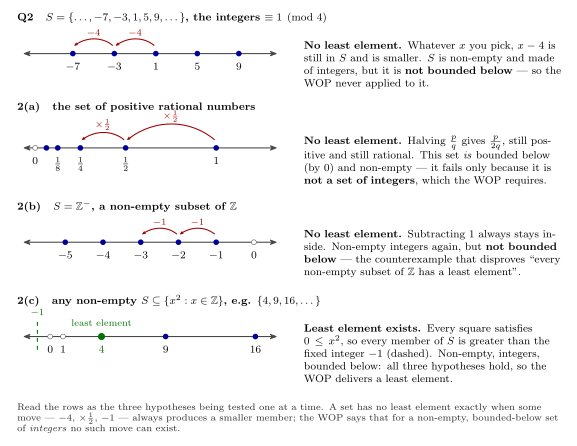
Figure 24: Four sets tested against the well-ordering principle, and which of its conditions each one fails. A set has no least element exactly when some move always produces a smaller member still inside it — subtract 4, halve, subtract 1 — and each disproof is the exhibition of that move. The rows are drawn to scale: the mod-4 and negative-integer sets march off to the left forever, while the positive rationals stay bounded below by 0 and fail for a different reason, having no integrality to stop them accumulating. Open circles mark numbers not in the set. Each hop arrow is labelled by its operation.
MI, SMI and the WOP on one example
The claim \(3 \mid a_n\), for the sequence \(a_n = a_{n-1} - a_{n-3}\) above, can be proved three times over — by SMI, by MI on the reworded predicate \(Q(n) \equiv P(0) \wedge P(1) \wedge \cdots \wedge P(n)\), and by the WOP taking the least counterexample. All three proofs share the same algebraic core, \(a_{k+1} = a_k - a_{k-2} = 3x - 3y = 3(x-y)\), and in the SMI and MI proofs that line is identical. They differ only in how the earlier cases are made available. All three are written out in strong-induction-and-the-well-ordering-principle.
Three details of those proofs, all recorded in that note:
- The MI proof’s basis step is \(n = 2\), not \(n = 0\), because \(Q(2)\) is the statement that packs all three of \(3 \mid a_0\), \(3 \mid a_1\), \(3 \mid a_2\) into one predicate.
- The MI proof’s last step concludes \(Q(k+1)\), not \(P(k+1)\). An induction run on \(Q\) must conclude \(Q(k+1)\).
- The WOP proof’s “least element \(k\)” is the least counterexample, which is the same information the strong inductive hypothesis carries, obtained a different way.
Worked: where the prime-factorisation proof uses the WOP
How does the following proof use the well-ordering principle for the integers?
Theorem: every integer \(n > 1\) can be written as a product of primes.
Proof: suppose the theorem is false. Then there exists an integer \(n > 1\) that is not a product of primes. Choose the smallest such number \(n\). Since \(n > 1\), then either \(n\) is prime or \(n\) is composite.
If \(n\) is prime, then \(n\) is a product of primes.
If \(n\) is composite, then \(n = rs\) for some positive integers \(r \neq 1\) and \(s \neq 1\). This implies that \(1 < r < n\) and \(1 < s < n\). Because we chose \(n\) to be the smallest integer that is not a product of primes, both \(r\) and \(s\) (which are smaller) are products of primes. Let \(r = p_1p_2\dots p_a\) and \(s = q_1q_2\dots q_b\) where the \(p_i\) and \(q_j\) are primes, and so \(n = rs = p_1p_2\dots p_a q_1q_2\dots q_b\) is a product of primes also.
In either case, \(n\) is a product of primes, contradicting our choice of \(n\). Therefore every integer \(n > 1\) can be written as a product of primes.
At the step “choose the smallest such number \(n\)” — that is the well-ordering principle, and nothing else in the proof invokes it. Written in full, the step reads “By the WOP we can choose the smallest such number \(n\)”. The proof has just established that the set of counterexamples is non-empty, and every member is an integer greater than 1, so the set is bounded below; the WOP is what licenses picking a least element out of it. Everything downstream (“because we chose \(n\) to be the smallest…”) depends on that element existing.
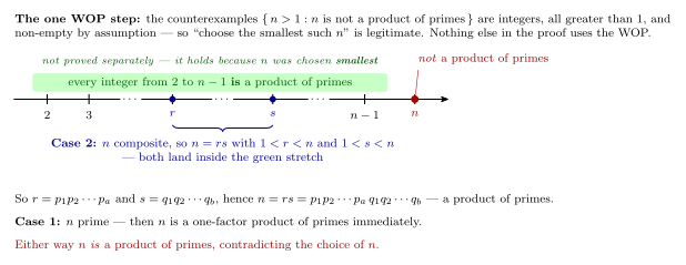
Figure 25: The well-ordering proof that every integer n > 1 is a product of primes, drawn on the number line: the well-ordering principle is used once, and everything after it lives off that one step. The green stretch is not proved — it holds only because n was chosen smallest, and the whole proof consists of showing that the two factors of a composite n land inside it. Compare the same shape in the well-ordering proof of 3 | a_n: least counterexample, a stretch below it that is known to be fine, and a descent that lands inside that stretch. The r and s ticks are placed arbitrarily inside the range, since the argument fixes only that 1 < r, s < n.
Set this next to the strong-induction proof of the same theorem above and the two are the same argument turned inside out. Strong induction builds up: assume \(P(2), \dots, P(k)\), prove \(P(k+1)\). The WOP version descends: assume some \(n\) fails, take the least such, and find that its factors — which are smaller, so they do not fail — hand you the very factorisation \(n\) was supposed to lack. The green stretch in the figure is doing the job that “\(P(2) \wedge \cdots \wedge P(k)\)” does in the induction.
Mathematical induction to prove a divisibility property
Recall that for integers \(n\) and \(d\) with \(d \neq 0\), \(d \mid n\) if and only if there exists some integer \(a\) such that \(n = da\) (see divisibility-and-factorisation).
Worked: \(5 \mid (7^n - 2^n)\)
Prove that for each integer \(n \geq 0\), \(5 \mid (7^n - 2^n)\).
Let \(P(n)\) be the predicate \(5 \mid (7^n - 2^n)\).
Basis step (\(P(0)\)). When \(n = 0\), \(7^n - 2^n = 7^0 - 2^0 = 1 - 1 = 0 = 5 \times 0\). Therefore \(5 \mid 0\), and so \(P(0)\) is true.
Inductive step (\(P(k) \to P(k+1)\)). Suppose \(P(k)\) is true for some \(k \geq 0\). Then \(5 \mid (7^k - 2^k)\), so there exists \(b \in \mathbb{Z}\) such that \(7^k - 2^k = 5b\). Thus \(7^k = 5b + 2^k\).
Consider \(P(k+1)\). Then
\[\text{LHS of } P(k+1) = 7^{k+1} - 2^{k+1} = 7\big(7^k\big) - 2\big(2^k\big)\] \[= 7\big(5b + 2^k\big) - 2\big(2^k\big) \qquad \text{(by the inductive hypothesis } P(k)\text{)}\] \[= 5(7b) + (7-2)2^k = 5\big(7b + 2^k\big)\]
Therefore \(5 \mid (7^{k+1} - 2^{k+1})\), so \(P(k) \to P(k+1)\). \(/\!/\)
Conclusion. By the principle of mathematical induction, \(5 \mid (7^n - 2^n)\) for each integer \(n \geq 0\).
The idea: separate \(7^k\) and \(2^k\) out of \(7^{k+1} - 2^{k+1}\), then use the inductive hypothesis to get rid of the \(7^k\). Replacing it with \(5b + 2^k\) is what makes a factor of 5 appear; the two \(2^k\) terms then collect into \((7-2)2^k\), which is another multiple of 5.
Two things about the shape of this one:
- Ordinary induction, not strong. Nothing here is a recurrence reaching back several terms — \(P(k+1)\) is built out of \(P(k)\) alone — so one base case is all it needs. It is the contrast to everything above it.
- The end mark and the conclusion. The double slash \(/\!/\) closes the inductive step at “\(P(k) \to P(k+1)\)”. The Conclusion line that follows, “by the principle of mathematical induction”, completes the course’s induction skeleton. (\(/\!/\) is an end-of-proof mark; \(\square\) and no mark at all are also used — see math1061-diagram-notation, which records four options as sanctioned.)
See also
- strong-induction-and-the-well-ordering-principle · mathematical-induction · sequences-and-summations · proof-techniques · divisibility-and-factorisation
- 2026-08-24-sequences-and-mathematical-induction — Lecture 13
- practice-problems — §18, with full worked solutions
Week 6
Lecture 15 — Mathematical Induction and Recursive Definitions
Pre-work: Video 019 (Recursive Definitions). See recursive-definitions for the reference material — what a recursive definition of a sequence or a set consists of, and the worked examples — and mathematical-induction / strong-induction-and-the-well-ordering-principle for the proof machinery used below.
Learning goals
- Continue to become more comfortable with mathematical induction.
- Become more familiar with recursive definitions of sequences and sets.
Worked: what is wrong with this ‘proof’ that all numbers are equal?
Proof. Let \(P(n)\) be the predicate “for any collection of \(n\) numbers, \(x_1, x_2, \dots, x_n\), it is always the case that \(x_1 = x_2 = \cdots = x_n\).”
Basis step: \(P(1)\) is true, since the collection is just \(x_1\).
Inductive step: Suppose that \(k\) is a positive integer and that \(P(k)\) is true. This means that in each collection of \(k\) numbers, all the numbers are equal.
Now consider a collection of \(k+1\) numbers, say \(x_1, x_2, \dots, x_k, x_{k+1}\).
The sub-collection \(x_1, x_2, \dots, x_k\) contains \(k\) numbers, and so \(x_1 = x_2 = \cdots = x_k\) by the inductive hypothesis.
The sub-collection \(x_2, x_3, \dots, x_{k+1}\) also contains \(k\) numbers, and so \(x_2 = x_3 = \cdots = x_{k+1}\) by the inductive hypothesis.
Therefore \(x_1 = x_2 = \cdots = x_k = x_{k+1}\) and so \(P(k+1)\) is true.
By mathematical induction, \(P(n)\) is true for each integer \(n \geq 1\), and so we have proven that all numbers are equal.
The conclusion is false, so something in the argument must fail.
The basis step is fine. So are “now consider a collection of \(k+1\) numbers” and the first sub-collection’s conclusion. The trouble is with the second sub-collection, \(x_2, \dots, x_{k+1}\). There are two readings of where it goes wrong; both turn on that sub-collection and they differ only over which line is at fault.
One reading puts the fault at the second use of the inductive hypothesis: if \(P(k)\) is a statement about \(x_1, \dots, x_k\), i.e. \(x_1 = x_2 = \cdots = x_k\), then concluding \(x_2 = x_3 = \cdots = x_{k+1}\) carries \(P(k)\) over to a different \(k\) numbers.
The other puts it one line later. \(P(n)\) as stated is about any collection of \(n\) numbers, and both sub-collections genuinely do contain \(k\) of them, so each conclusion is defensible taken alone; what cannot be defended is the “Therefore” line, at \(k = 1\). Gluing \(x_1 = \cdots = x_k\) to \(x_2 = \cdots = x_{k+1}\) into one chain requires the two sub-collections to overlap — you need some number that appears in both, to carry the equality across. For \(k \geq 2\) they share \(x_2, \dots, x_k\) and the step is sound. For \(k = 1\) the collection is just \(x_1, x_2\), the two sub-collections are \(\{x_1\}\) and \(\{x_2\}\), and they share nothing: each says only that a single number equals itself, and there is no reason at all that \(x_1 = x_2\).
Put the two sub-collections on one row and the overlap is visible: \(x_1, \dots, x_k\) (orange in the figure) and \(x_2, \dots, x_{k+1}\) (yellow), the second leaving out \(x_1\). What matters is what the two share.
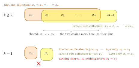
Figure 26: Why the inductive step fails at \(k = 1\). The two sub-collections of the \(k+1\) numbers are drawn as overlapping rings on a single row, the first in orange and the second in yellow, so the shared elements can be seen at once. For \(k \geq 2\) they overlap on \(x_2, \dots, x_k\), and that shared block is exactly what lets the two equality chains be joined into one. For \(k = 1\) the rings shrink to \({x_1}\) and \({x_2}\), they share nothing, and nothing in the argument forces \(x_1 = x_2\).
So \(P(1) \to P(2)\) is false. The chain of implications never gets off the basis step, and the “proof” proves nothing beyond \(P(1)\).
The lesson: the inductive step has to hold for every \(k\) from the basis value on — including the very first one. An inductive step that is valid for all large \(k\) but fails at the bottom leaves a gap the induction cannot cross.
Recursively defined sequences
A recursive definition needs initial conditions and a recurrence relation — and the same recurrence relation with different initial conditions can give a completely different sequence (\(a_1 = 2\), \(a_k = 3a_{k-1}\) gives \(2, 6, 18, 54, \dots\); \(b_1 = 7\) with the same recurrence gives \(7, 21, 63, 189, \dots\)). See recursive-definitions.
Number the two parts in the order you use them: (i) initial conditions, (ii) recurrence relation. The numbering comes back in 2026-08-31-solving-recurrence-relations, where the two things Method 1 checks are labelled (i) and (ii) because they are exactly these two halves.
Worked: which recurrence does \(b_n = 4n + 3\) satisfy? (pre-class Q2)
Which of the following recurrence relations is satisfied by the sequence \(b_n = 4n + 3\) for each integer \(n \geq 1\)?
b. \(b_k = 4 + b_{k-1}\) for each integer \(k \geq 2\).
The method: assume \(b_{k-1} = 4(k-1) + 3\), check what \(b_k\) equals — that is, \(P(k-1) \Rightarrow P(k)\) — for each candidate in turn. The target is \(b_k = 4k + 3\).
| Option | Substituting \(b_{k-1} = 4(k-1)+3\) | |
|---|---|---|
| a. \(b_k = 4b_{k-1}\) | \(4\big(4(k-1)+3\big) = 16k - 16 + 3 = 16k - 13\) | ✗ |
| b. \(b_k = 4 + b_{k-1}\) | \(4 + 4(k-1) + 3 = 4k + 3\) | ✓ |
| c. \(b_k = 3 + b_{k-1}\) | \(3 + 4(k-1) + 3 = 4k + 2\) | ✗ |
| d. \(b_k = 3b_{k-1}\) | \(3\big(4(k-1)+3\big) = 12k - 3\) | ✗ |
Worked: the recursive definition of \(c_n = 3^n - 2^n\) (pre-class Q3)
The sequence \(c_n = 3^n - 2^n\) for each integer \(n \geq 1\) satisfies the recurrence relation \(c_k = 5c_{k-1} - 6c_{k-2}\) for each integer \(k \geq 3\). What is the recursive definition for this sequence?
c. \(c_1 = 1\), \(c_2 = 5\), \(c_k = 5c_{k-1} - 6c_{k-2}\) for each integer \(k \geq 3\).
Two things pin it down: the values of the initial conditions, and the indexing.
The initial conditions come from evaluating the explicit formula:
\[c_1 = 3^1 - 2^1 = 3 - 2 = 1 \qquad c_2 = 3^2 - 2^2 = 9 - 4 = 5\]
Option c has those two values. Option b has the clashing \(c_1 = 0\) — so b goes out on values. Options a and d go out on indexing instead: they define \(c_0\) and start the recurrence at \(k \geq 2\), whereas the sequence was given as starting at \(n = 1\), so \(c_0\) lies outside its domain. Option d fails on values too — it puts \(c_1 = 5\).
Option a is the subtle one. Its arithmetic is entirely correct — \(c_0 = 3^0 - 2^0 = 0\), \(c_1 = 1\), and \(c_2 = 5(1) - 6(0) = 5\), \(c_3 = 5(5) - 6(1) = 19 = 3^3 - 2^3\) — so it does generate the right sequence for every \(n \geq 1\). It is wrong only because it defines a term the given sequence does not have. That is the difference between a wrong sequence and a right sequence with the wrong domain.
Worked: a recursive definition for \(a_n = (-1)^n / n!\)
Consider the sequence defined by the explicit formula \(a_n = \dfrac{(-1)^n}{n!}\) for each integer \(n \geq 0\). (Recall that for \(n \in \mathbb{Z}^{+}\), \(n! = n(n-1)\cdots(2)(1)\), and that \(0! = 1\) by definition. Memorise that clause: it is what makes a formula built out of \(n!\) work at \(n = 0\) with no special case, which is exactly what this sequence needs.)
(a) Determine the first five terms of this sequence and guess a suitable recurrence relation.
\[a_0 = \frac{(-1)^0}{0!} = \frac{1}{1} = 1 \qquad a_1 = \frac{(-1)^1}{1!} = \frac{-1}{1} = -1 \qquad a_2 = \frac{(-1)^2}{2!} = \frac{1}{2}\] \[a_3 = \frac{(-1)^3}{3!} = \frac{-1}{3 \times 2} = -\frac{1}{6} \qquad a_4 = \frac{(-1)^4}{4!} = \frac{1}{4 \times 3 \times 2} = \frac{1}{24}\]
The guess does not come from staring at the five values; it comes from asking what multiplies each one to give the next. Write those multipliers in as curved arrows between consecutive terms:
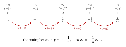
Figure 27: Reading the recurrence off the terms. Each curved arrow carries the factor taking one term to the next, and the four factors \(-1, -\tfrac12, -\tfrac13, -\tfrac14\) are read as one pattern, \(-\tfrac1n\) at step \(n\). The pattern is the guess; part (b) is where it gets proved.
\[a_n = -\frac{1}{n}a_{n-1}\]
(b) Show that this sequence satisfies your recurrence relation.
Suppose \(a_{n-1} = \dfrac{(-1)^{n-1}}{(n-1)!}\). Then
\[a_n = -\frac{1}{n}\cdot a_{n-1} = \frac{(-1)(-1)^{n-1}}{n \cdot (n-1)!} = \frac{(-1)^n}{n!} \qquad \square\]
(c) Write down a recursive definition of this sequence.
- initial condition: \(a_0 = 1\)
- recurrence relation: \(a_n = -\dfrac{1}{n}a_{n-1}\) for all \(n \geq 1\)
A recursively defined set
Three parts — Base, Recursion and Restriction — spelled out in recursive-definitions along with the set of all binary strings \(B\), in which the string 011 is built up as \(\varepsilon \to 0 \to 01 \to 011\). The worked question below is practice with step II, the Recursion: what its rules do and do not generate.
Worked: which strings are in \(S\)?
Let the subset \(S\) of the set of all binary strings be defined recursively as follows. Base: the empty string is in \(S\). Recursion: if \(s \in S\), then \(s1 \in S\) and \(s01 \in S\). Restriction: nothing is in \(S\) other than objects defined by the Base and the Recursion.
So there are two rules, named by what they append: rule 1 (append 1) and rule 01 (append 01). Naming them matters, because a membership argument is a chain of rule applications and each link has to say which rule was used. The rule’s bare name goes above the arrow, and nothing else:
(a) Is the string 1101 \(\in S\)?
Yes — it has a build history:
\[\varepsilon \;\xrightarrow{\;1\;}\; 1 \;\xrightarrow{\;1\;}\; 11 \;\xrightarrow{\;01\;}\; 1101 \in S\]
(b) Is the string 0110 \(\in S\)?
No — \(S\) contains no strings ending in 0. Both rules append a string ending in 1, so every non-empty member of \(S\) ends in 1, and by the Restriction there is nothing else in \(S\).
(c) Is the string 1001 \(\in S\)?
No — \(S\) contains no strings with two or more consecutive 0s. A 0 can only ever enter as the first character of an appended 01, so every 0 is immediately followed by a 1.
(d) State a property that all strings in \(S\) must have and explain why.
The number of 1s is greater than or equal to the number of 0s.
The empty string has zero of each, so the property holds at the Base. Each rule preserves it: appending 1 adds one 1 and no 0s, and appending 01 adds one of each. So no application of the Recursion can ever make the 0s outnumber the 1s, and by the Restriction every member of \(S\) is reached by some finite chain of these rules.
Worked: \(F_n < 2^n\) for the Fibonacci sequence
Recall the Fibonacci sequence: \(F_0 = 1\), \(F_1 = 1\), \(F_k = F_{k-1} + F_{k-2}\) for every integer \(k \geq 2\). Use (strong) mathematical induction to prove that \(F_n < 2^n\) for every integer \(n \geq 1\).
The first thing to settle is the number of base cases. The recurrence \(F_k = F_{k-1} + F_{k-2}\) points to 2 base cases; the “\(n \geq 1\)” in the claim points to 1 base case. The recurrence settles it. \(F_k = F_{k-1} + F_{k-2}\) reaches back two terms, so producing \(P(k+1)\) needs \(P(k)\) and \(P(k-1)\): that is strong induction, and it needs two base cases to start from.
The same reasoning fixes the range of the inductive step: it is \(\forall k \geq 2\), not \(\forall k \geq 1\). At \(k = 1\) the step would reach for \(P(0)\), which is not one of the base cases. This is not merely an indexing nicety, because with \(F_0 = 1\) the statement \(P(0)\) is false — it would say \(F_0 < 2^0\), i.e. \(1 < 1\). So the claim could not have been extended down to \(n = 0\) in any case.
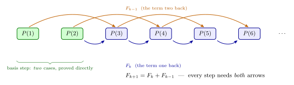
Figure 28: The shape of the strong induction, drawn out. Each \(P(k+1)\) is reached from the term one back (blue) and the term two back (orange), because the recurrence \(F_{k+1} = F_k + F_{k-1}\) names both; that is why the inductive hypothesis has to be the strong one, and why two cases have to be proved outright before the chain can start.
Let \(P(n)\) be the predicate \(F_n < 2^n\).
Basis step — \(P(1)\) and \(P(2)\).
LHS of \(P(1)\): \(F_1 = 1\). RHS of \(P(1)\): \(2^1 = 2\). Since \(1 < 2\), \(P(1)\) is true.
LHS of \(P(2)\): \(F_2 = F_1 + F_0 = 1 + 1 = 2\). RHS of \(P(2)\): \(2^2 = 4\). Since \(2 < 4\), \(P(2)\) holds.
Inductive step — \(\big(P(1), \dots, P(k)\big) \to P(k+1)\) for all \(k \geq 2\).
LHS of \(P(k+1)\):
\[F_{k+1} = F_k + F_{k-1} < 2^k + 2^{k-1} \qquad \text{(by the inductive hypothesis } P(k) \text{ and } P(k-1)\text{)}\] \[= 2\big(2^{k-1}\big) + 2^{k-1} = 3\big(2^{k-1}\big) < 2^2\big(2^{k-1}\big) \qquad (3 < 4 = 2^2)\] \[= 2^{k+1}\]
which is the RHS of \(P(k+1)\). Therefore \(\big(P(1), \dots, P(k)\big) \to P(k+1)\). \(\square\)
The trick in the middle is rewriting \(2^k\) as \(2(2^{k-1})\) so that both terms carry the same power and can be collected — turning \(2^k + 2^{k-1}\) into \(3(2^{k-1})\), which is then bounded by \(4(2^{k-1}) = 2^{k+1}\).
See also
- recursive-definitions · mathematical-induction · strong-induction-and-the-well-ordering-principle · sequences-and-summations
- 2026-08-27-strong-induction-and-well-ordering — Lecture 14
- practice-problems — §19 Recursive Definitions, with full worked solutions
Lecture 16 — Solving Recurrence Relations
Pre-work: Video 020 (Solving Recurrence Relations). See solving-recurrence-relations for the reference material — arithmetic and geometric sequences, the two proof methods and the Tower of Hanoi — and recursive-definitions for the definitions this lecture starts from.
Learning goals
- Become more familiar with recursive definitions of sequences.
- Gain fluency in moving between a recursive definition and an explicit formula.
Why the second goal is worth having
Put the two forms side by side and ask for the same thing from each, say the term at \(n = 1000\):
| Form | Example | Getting \(a_{1000}\) |
|---|---|---|
| Explicit formula | \(a_n = 7n^2\) for all \(n \in \mathbb{Z}^{+}\) | substitute: \(7(1000)^2\) — one step |
| Recursive definition | \(a_0 = 4\) and \(a_n = 5a_{n-1} + 3\) | compute \(a_1, a_2, \dots\) all the way up — a thousand steps |
That gap is the motivation for the whole topic. A recursive definition is often the easy thing to write down (it is how the Tower of Hanoi and the Fibonacci numbers naturally arise), and an explicit formula is the thing you want to compute with. The topic is converting the first into the second.
Calculating terms gives a guess, not a proof
To show that a recursive definition is the same as an explicit formula, it is not enough to calculate values and show they give the same terms. Calculating terms produces a guess, never a proof. Any finite run of terms is consistent with infinitely many formulas (see sequences-and-summations), so agreement on the first five terms says nothing about the sixth. Terms are calculated to have something to prove. In the two methods below, “write out the first few terms and guess” is a separate step from “prove that your guess is correct”.
Question 3 of the pre-class work asks whether such a claim is true or false. It is worked below, twice, once by each method.
Arithmetic and geometric sequences
For a sequence \(a_0, a_1, a_2, \dots\):
| Recurrence relation | Explicit formula | |
|---|---|---|
| Arithmetic | \(a_k = a_{k-1} + d\) for integers \(k \geq 1\) | \(a_n = a_0 + dn\) for integers \(n \geq 0\) |
| Geometric | \(a_k = r \cdot a_{k-1}\) for integers \(k \geq 1\) | \(a_n = a_0 \cdot r^{\,n}\) for integers \(n \geq 0\) |
The four formulas look alike. The two written in \(k\) with \(a_{k-1}\) on the right are the recurrence relations; the two written in \(n\) are the explicit formulas.
For example, \(2, 6, 18, 54, \dots\) multiplies by \(3\) each step, so \(r = 3\), and with \(a_0 = 2\) the explicit formula is \(a_n = 2 \cdot 3^{\,n}\).
Worked: geometric but not arithmetic
The three terms \(\tfrac{5}{8}, \tfrac{5}{2}, 10\) could be three consecutive terms of what type of sequence?
A geometric sequence. Putting them over a common denominator, \(\tfrac{5}{8}, \tfrac{20}{8}, \tfrac{80}{8}\), makes both tests quick. Run both on the same three terms, with the differences above the row and the ratios below it:
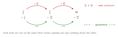
Figure 29: Both tests, run on the same three terms. Rewriting over the common denominator \(8\) makes each test one subtraction or one division. The differences \(\tfrac{15}{8}\) and \(\tfrac{60}{8}\) disagree, so the terms are not arithmetic; the ratios are both \(4\), so they are geometric with \(r = 4\). Neither verdict is evidence about the other, which is what the answer both gets wrong.
The answer “both” is the trap. Passing the ratio test earns nothing on the difference test. The two conditions are independent.
Worked: both arithmetic and geometric
The three terms \(2, 2, 2\) could be three consecutive terms of what type of sequence?
Both. The differences are all \(0\) (arithmetic, \(d = 0\)) and the ratios are all \(1\) (geometric, \(r = 1\)).
This is a constant sequence, \(a_n = c\) for all \(n \in \mathbb{Z}^{+}\). The constant sequences are not just examples of the overlap but the whole of it — \(a_n = a_0 + dn\) and \(a_n = a_0 r^{\,n}\) can agree for every \(n\) only when \(d = 0\) and the sequence is constant.
From a recursive definition to an explicit formula
Given a recursive definition, write out the first few terms and guess an explicit formula. To prove the guess correct, either:
Method 1. Check that your guess gives the correct initial conditions and satisfies the recurrence relation.
Method 2. Use (strong) mathematical induction to prove that if \(a_0, a_1, a_2, \dots\) is the sequence defined by [the recursive definition], then [your guess].
Method 1 is the quicker one and Method 2 the rigorous one. Both are complete proofs; Method 1 leans on the fact that a recursive definition determines its sequence uniquely, which solving-recurrence-relations spells out.
Q3 of the pre-class questions
True or false? The sequence defined recursively as \(c_1 = 1\) and \(c_k = c_{k-1} + 2^k\) for each integer \(k \geq 2\) can be defined using the explicit formula \(c_n = 2^{\,n+1} - 3\) for each integer \(n \geq 1\).
True.
By Method 1
Label the two checks (i) and (ii). They are the two halves of the recursive definition.
(i) Initial conditions \((n=1)\): \(\;c_1 = 2^{1+1} - 3 = 2^2 - 3 = 4 - 3 = 1\) ✓
(ii) Recurrence relation:
\[\text{LHS} = c_k = 2^{k+1} - 3\] \[\text{RHS} = c_{k-1} + 2^k = 2^{(k-1)+1} - 3 + 2^k = 2^k + 2^k - 3 = 2\big(2^k\big) - 3 = 2^{k+1} - 3\]
so the explicit formula satisfies the given recurrence relation. Therefore the statement is true.
By Method 2
To prove that if \(c_1, c_2, c_3, \dots\) is the sequence defined by \(c_1 = 1\) and \(c_k = c_{k-1} + 2^k\) for each integer \(k \geq 2\), then \(c_n = 2^{\,n+1} - 3\) for each integer \(n \geq 1\) — by mathematical induction (PMI).
Let \(P(n)\) be the predicate \(c_n = 2^{\,n+1} - 3\).
Basis step. \(c_1 = 1\) by the recursive definition, and \(2^{1+1} - 3 = 4 - 3 = 1\), so the statement is true for \(n = 1\).
Inductive hypothesis. Suppose \(P(k)\) is true for some integer \(k \geq 1\). This means \(c_k = 2^{k+1} - 3\). Then
\[c_{k+1} = c_k + 2^{k+1} = 2^{k+1} - 3 + 2^{k+1} = 2\big(2^{k+1}\big) - 3 = 2^{k+2} - 3\]
Therefore \(P(k+1)\) is true. Hence by mathematical induction the sequence with the given recursive definition is defined explicitly as \(c_n = 2^{\,n+1} - 3\) for each integer \(n \geq 1\). \(\blacksquare\)
The recurrence is stated for \(k \geq 2\), so the substitution \(c_{k+1} = c_k + 2^{k+1}\) is legitimate for \(k \geq 1\) — the indices line up exactly with the basis step.
Worked: a recurrence with two initial conditions
Consider the sequence \(b_0 = 0\), \(b_1 = 1\) and \(b_k = \tfrac{1}{2}\big(b_{k-1} + b_{k-2} + 1\big) + 3(k-1)\) for each integer \(k \geq 2\).
(a) Calculate a few more terms and guess an explicit formula
\[b_2 = \tfrac{1}{2}(b_1 + b_0 + 1) + 3(1) = \tfrac{1}{2}(0 + 1 + 1) + 3 = 1 + 3 = 4\] \[b_3 = \tfrac{1}{2}(4 + 1 + 1) + 3(2) = 3 + 6 = 9\] \[b_4 = \tfrac{1}{2}(9 + 4 + 1) + 3(3) = 7 + 9 = 16\]
giving \(0, 1, 4, 9, 16, \dots\) — guess \(b_n = n^2\) for all integers \(n \geq 0\).
(b) Prove the guess by Method 1
Initial conditions \((n = 0\) and \(n = 1)\): \(\;b_0 = 0^2 = 0\) ✓ and \(b_1 = 1^2 = 1\) ✓ — so the explicit formula satisfies the initial conditions. Two initial conditions means two checks.
Recurrence relation. Suppose \(b_n = n^2\) for all \(n\):
\[\text{LHS} = b_k = k^2\]
\[\begin{aligned} \text{RHS} &= \tfrac{1}{2}\big((k-1)^2 + (k-2)^2 + 1\big) + 3(k-1) \\ &= \tfrac{1}{2}\big(k^2 - 2k + 1 + k^2 - 4k + 4 + 1\big) + 3k - 3 \\ &= \big(k^2 - 3k + 3\big) + 3k - 3 \\ &= k^2 \end{aligned}\]
\(\therefore\) LHS \(=\) RHS, so the explicit formula satisfies the recurrence relation. \(\blacksquare\)
The same result can be proved by strong induction — strong because the recurrence reaches back two terms, so \(P(k)\) alone would not be enough. See solving-recurrence-relations for that proof written out.
(c) Find a different recursive definition of the sequence
Look for a one-step recurrence \(b_n = b_{n-1} + p\) and solve for the step:
\[n^2 = (n-1)^2 + p \;\implies\; p = 2n - 1 \;\implies\; b_n = b_{n-1} + (2n-1)\]
Completed into a recursive definition, \(b_0 = 0\) with \(b_n = b_{n-1} + (2n-1)\) for \(n \geq 1\) gives the same sequence — the squares as running totals of the odd numbers. Two things to take from the exercise: a sequence does not have a unique recursive definition, and this one needs only one initial condition where the original needed two.
Worked: a recurrence with a fraction
Consider the sequence defined as \(d_0 = 1\) and \(d_k = \dfrac{d_{k-1}}{1 + d_{k-1}}\) for each integer \(k \geq 1\).
(a) Calculate a few more terms and guess an explicit formula
The trick used throughout is “\(\times 1\)”: multiply top and bottom by the denominator of the inner fraction to clear the compound fraction in one move.
\[d_1 = \frac{1}{1+1} = \frac{1}{2} \qquad d_2 = \frac{\tfrac{1}{2}}{1 + \tfrac{1}{2}} \cdot \frac{2}{2} = \frac{1}{2+1} = \frac{1}{3} \qquad d_3 = \frac{\tfrac{1}{3}}{1 + \tfrac{1}{3}} \cdot \frac{3}{3} = \frac{1}{3+1} = \frac{1}{4}\]
giving \(1, \tfrac12, \tfrac13, \tfrac14, \dots\) — guess \(d_n = \dfrac{1}{n+1}\).
(b) Prove the guess by Method 1
Initial condition \((d_0 = 1)\): \(\;d_0 = \dfrac{1}{0+1} = \dfrac{1}{1} = 1\) ✓
Recurrence relation. Suppose \(d_n = \dfrac{1}{n+1}\):
\[\text{LHS} = d_k = \frac{1}{k+1} \qquad\qquad \text{RHS} = \frac{d_{k-1}}{1 + d_{k-1}} = \frac{\tfrac{1}{k}}{1 + \tfrac{1}{k}} \cdot \frac{k}{k} = \frac{1}{k+1}\]
\(\therefore\) LHS \(=\) RHS, so the explicit formula satisfies the recurrence relation. \(\blacksquare\)
The same result can be proved by ordinary induction (MI) — ordinary this time, since the recurrence reaches back only one term.
The Tower of Hanoi
Given a tower of 8 discs in decreasing size on one of three pegs, transfer the entire tower to one of the other pegs, subject to: (a) move only one disc at a time; (b) never move a larger disc onto a smaller disc. Is there a solution? If so, what is the fewest number of moves?
For \(n \geq 1\) let \(m_n\) be the minimum number of moves to transfer a tower of \(n\) discs from one pole to another. Work up to the recurrence through three cases:
- \(n = 1\): one move, so \(m_1 = 1\).
- \(n = 2\): small disc to the spare peg, large disc across, small disc back on top — so \(m_2 = 3\).
- the general case: the whole transfer takes \(m_n\) moves and passes through four board positions, with the \(n-1\) smaller discs treated as one group. For four discs, \(m_4 = m_3 + 1 + m_3\).
The first two are shown below as sequences of board positions, each a transfer that takes that many moves. The recurrence is read off the general case.
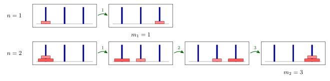
Figure 30: The two small cases. One disc goes left peg to right peg in one move, and two discs take three, numbered \(1, 2, 3\), with the small disc parked on the middle peg in between. Each position is boxed and the green arrows are the moves. The middle move is forced: the large disc cannot move until the small one is off it and cannot land on the small one, so the spare peg has to be used, and that is what generalises to \(m_k = 2m_{k-1} + 1\).
In general:
\[m_1 = 1 \qquad\text{and}\qquad m_k = 2m_{k-1} + 1 \;\text{ for all integers } k \geq 2\]
The three stages between the four board positions take \(m_{n-1}\), \(m_1 = 1\) and \(m_{n-1}\) moves (drawn out in solving-recurrence-relations). The largest disc has to move at some point, and it can only move onto an empty peg — so the other \(k-1\) discs must first be stacked on the spare peg, and then moved back on top afterwards. Two sub-transfers plus one move.
Worked: proving the Tower of Hanoi formula
On page 310 (4th edition) or page 346 (5th edition) the textbook guesses \(m_n = 2^n - 1\) for all integers \(n \geq 1\). Prove the guess is correct by checking that it gives the correct initial conditions and satisfies the recurrence relation.
Suppose \(m_n = 2^n - 1\) for all \(n \in \mathbb{Z}^{+}\).
Initial condition \((m_1 = 1)\): \(\;m_1 = 2^1 - 1 = 2 - 1 = 1\) ✓
Recurrence relation \((m_k = 2m_{k-1} + 1)\):
\[\text{LHS} = m_k = 2^k - 1\] \[\text{RHS} = 2m_{k-1} + 1 = 2\big(2^{\,k-1} - 1\big) + 1 = 2 \cdot 2^{\,k-1} - 2 + 1 = 2^k - 1\]
So LHS \(=\) RHS \(\therefore\) the explicit formula satisfies the recurrence relation. \(\blacksquare\)
The textbook proves the same result by mathematical induction (PMI) instead — so this is Method 1 versus Method 2 on the same problem one more time.
The eight-disc puzzle of the problem statement needs \(2^8 - 1 = 255\) moves, and “is there a solution?” is answered constructively, because the recurrence is the algorithm.
See also
- solving-recurrence-relations — the reference note for all of the above
- recursive-definitions · sequences-and-summations · mathematical-induction · strong-induction-and-the-well-ordering-principle
- 2026-08-31-recursive-definitions — Lecture 15
- 2026-09-03-set-theory-definitions — Lecture 17
- practice-problems — §20 Solving Recurrence Relations, with full worked solutions
Lecture 18 — Proving Properties of Sets and Intro to Functions
Pre-work: Video 023 (Properties of sets) and Video 024 (Functions defined on general sets). See proving-set-properties for the three proof methods and the set identities, and functions-on-general-sets for the function material in the second half.
Learning goals
- Be comfortable with notation for sets including \(x \in A\), \(A \subseteq B\), \(A \subset B\), \(A \cap B\), \(A \cup B\), \(A - B\), \(A^{c}\), \(\mathcal{P}(A)\), \(A \times B\).
- Be able to use the element method to prove set properties.
- Be able to use the laws of logical equivalence to prove that two sets are equal.
- Be able to use set identities to prove that two sets are equal.
- Understand what a function is, and associated concepts and definitions.
Goal 1 carries over from 2026-09-03-set-theory-definitions. For goal 2, the element method, the operational point is that \(A = B\) means \((A \subseteq B\) and \(B \subseteq A)\) — the shape every equality proof below takes.
Common questions
Q1 and Q3 from video 23, and Q1 and Q2 from video 24, are all worked below.
What is the difference between co-domain and range, and how do you distinguish between them? The co-domain is declared, the range is computed. See the functions section.
Worked: Q1 from video 23 — a proper subset
Let \(S = \{x \in \mathbb{Z} \mid x \equiv 2 \;(\mathrm{mod}\; 3)\}\) and let \(T = \{x \in \mathbb{Z} \mid x \equiv 5 \;(\mathrm{mod}\; 6)\}\).
\[S = \{\dots, -7, -4, -1, 2, 5, 8, 11, \dots\} \qquad T = \{\dots, -7, -1, 5, 11, \dots\}\]
Prove that \(T \subset S\). The proof splits into the two things \(\subset\) demands, (i) and (ii):
(i) \(T \subseteq S\). Suppose \(t \in T\). Then \(t = 6k + 5\) for some integer \(k\). Thus \(t = 3(2k+1) + 2\), and since \(2k + 1 \in \mathbb{Z}\), we have \(t \in S\). Therefore \(T \subseteq S\).
(ii) \(T \neq S\) and \(\exists s \in S - T\). Furthermore, \(2 \in S\) but \(2 \notin T\), so \(T \subset S\). \(\blacksquare\)
Part (i) is the general argument — “suppose \(t \in T\)”, nothing assumed beyond membership. Part (ii) is a single witness. A universal claim needs a general argument; an existential claim needs one example, and mixing up which is which is the usual way this proof goes wrong.
Worked: Q3 from video 23 — a Venn diagram is not a proof
For all sets \(A\), \(B\), \(C\): \(\;(A - B) \cap (B - A) = \emptyset\). True.
Three Venn diagrams — \(A\) and \(B\); then \(A - B\) shaded; then \(B - A\) shaded — show the result, but they are not a proof. The figure is in proving-set-properties.
Worth taking seriously, because the diagrams are so convincing. A Venn diagram shows one configuration; the claim is about all sets, including the cases the picture does not draw — \(A = B\), either set empty, one contained in the other. And the regions are drawn non-empty when the statement has to survive them being empty.
The proof takes two lines: suppose \(x \in (A-B) \cap (B-A)\); then \(x \in A\) and \(x \notin B\), and also \(x \in B\) and \(x \notin A\); so \(x \in B\) and \(x \notin B\), a contradiction. Hence no such \(x\), and the intersection is empty. \(\blacksquare\)
Diagrams to find the answer; the element method to justify it.
The element method of proof
To prove that \(S \subseteq T\), you consider an arbitrary element \(x \in S\) and show that \(x \in T\).
To prove that \(S \subset T\), you prove that \(S \subseteq T\) and then prove \(\exists\, t \in T\) such that \(t \notin S\).
To prove that \(S = T\), you prove that \(S \subseteq T\) and also prove that \(T \subseteq S\).
Worked: complementation reverses containment
Prove that for all sets \(A\) and \(B\) in some universe \(U\), if \(A \subseteq B\) then \(B^{c} \subseteq A^{c}\).
Proof. Let \(x \in B^{c}\). Then \(x \in U - B\) (by definition of complement). Thus \(x \in U\) and \(x \notin B\) (by definition of set difference).
Since \(A \subseteq B\) we have: every element in \(A\) is also an element of \(B\). Taking the contrapositive, \[x \notin B \;\longrightarrow\; x \notin A\] Since \(x \in U\) and \(x \notin A\), then by the definition of complement, \(x \in A^{c}\). \(\blacksquare\)
The step to notice is the contrapositive. \(A \subseteq B\) gives you “\(x \in A \rightarrow x \in B\)”, which is the wrong way round for what you have; flipping it to “\(x \notin B \rightarrow x \notin A\)” is what makes the hypothesis usable. See proof-techniques for why that flip is free.
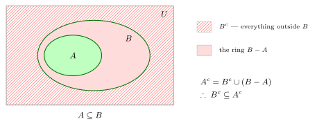
Figure 31: The universe as a rectangle, A inside B, and B-complement hatched in red. The shading of the ring B − A is what makes the result readable off the picture: A-complement is the hatched region plus the ring, so it contains B-complement. A picture like this is a check on the answer, not a substitute for the element proof above.
The result itself is worth remembering as a fact: complementation reverses containment. The smaller set has the bigger complement.
Methods of proof for properties of sets
Three methods, and when each is useful:
| Method | Useful for | Note |
|---|---|---|
| The element method | a variety of results about sets | the only one that can prove a containment, not just an equality |
| Laws of logical equivalence | proving two sets are equal | quicker |
| Set identities | proving two sets are equal | quicker |
The element method has three sub-forms, the second of which does not mention a second set at all:
- To prove \(S \subseteq T\), suppose \(x \in S\) and then prove that \(x \in T\).
- To prove that all elements in a set \(S\) have property \(P\), suppose \(x \in S\), and then prove that \(x\) has property \(P\).
- To prove that \(S = T\), first prove that \(S \subseteq T\), and then prove that \(T \subseteq S\).
The laws of logical equivalence method
Example. Prove that for all sets \(A\) and \(B\), \(\;A - (A - B) = A \cap B\).
\[\begin{aligned} x \in A - (A - B) &\equiv (x \in A) \land \big(x \notin (A-B)\big) && \text{by definition of set difference} \\ &\equiv (x \in A) \land \sim\!\big(x \in (A-B)\big) && \text{by definition of } \notin \\ &\equiv (x \in A) \land \sim\!\big((x \in A) \land (x \notin B)\big) && \text{by definition of set difference} \\ &\equiv (x \in A) \land \big(\sim\!(x \in A) \lor \sim\!(x \notin B)\big) && \text{by De Morgan's law} \\ &\equiv (x \in A) \land \big((x \notin A) \lor (x \in B)\big) && \text{by definition of } \in \text{ and } \notin \\ &\equiv \big((x \in A) \land (x \notin A)\big) \lor \big((x \in A) \land (x \in B)\big) && \text{by the distributive law} \\ &\equiv \mathbf{c} \lor \big((x \in A) \land (x \in B)\big) && \text{by the negation law} \\ &\equiv (x \in A) \land (x \in B) && \text{by the identity law} \\ &\equiv x \in A \cap B && \text{by the definition of } \cap \end{aligned}\]
The justifications are of two kinds, and the grouping is the lesson. Four of the nine lines are laws of logical equivalence doing the actual work — De Morgan, distributive, negation, identity. The other five are definitions of set symbols, translating in and out of logic: the three at the top, the last one, and — easy to miss — the “\(\in\) and \(\notin\)” line sitting in the middle of the chain, so the two kinds do not fall into neat blocks. Every line is named; the naming is where the marks are.
Because the chain is all \(\equiv\), this proves the equality in one pass rather than the element method’s two containments.
Set identities
The full table is in proving-set-properties and appears on the exam formula page (see formula-sheet). The ones used below:
| 3(b) | Distributive | \(A \cap (B \cup C) = (A \cap B) \cup (A \cap C)\) |
| 4(a) | Identity | \(A \cup \emptyset = A\) |
| 5(b) | Complement | \(A \cap A^{c} = \emptyset\) |
| 6 | Double Complement | \((A^{c})^{c} = A\) |
| 9(b) | De Morgan’s | \((A \cap B)^{c} = A^{c} \cup B^{c}\) |
| 12 | Set Difference | \(A - B = A \cap B^{c}\) |
Worked: the same equality by set identities
Using the set identities, prove that for all sets \(A\) and \(B\), \(\;A - (A - B) = A \cap B\).
The same result as the worked example, by the third method:
\[\begin{aligned} A - (A - B) &= A - (A \cap B^{c}) && \text{by the set difference law (12)} \\ &= A \cap (A \cap B^{c})^{c} && \text{by the set difference law (12)} \\ &= A \cap \big(A^{c} \cup (B^{c})^{c}\big) && \text{by De Morgan (9b)} \\ &= A \cap (A^{c} \cup B) && \text{by the double complement law} \\ &= (A \cap A^{c}) \cup (A \cap B) && \text{by the distributive law (3b)} \\ &= \emptyset \cup (A \cap B) && \text{by the complement law (5b)} \\ &= A \cap B && \text{by the identity law (4a)} \end{aligned}\]
Seven lines against the previous method’s nine, with no logic notation. Two things worth pulling out:
- Law 12 is applied twice — to the inner difference, then the outer one. Clearing every minus sign first is what makes the rest routine, since none of the other identities mention set difference at all.
- The final step cites identity law (4a), \(A \cup \emptyset = A\), but is applied to \(\emptyset \cup (A \cap B)\) — the operands reversed. Commutativity (1a) is being used silently. Standard practice, but the step is really two.
Russell’s paradox
When mathematicians wanted to show that all of mathematics could be built on set theory, Bertrand Russell discovered a problem.
Let \(S\) be the set of all sets that are not elements of themselves, \(S = \{A \mid A \text{ is a set and } A \notin A\}\). Is \(S\) an element of itself?
If \(S \in S\), then \(S \notin S\). If \(S \notin S\), then \(S \in S\). So we conclude that both \(S \in S\) and \(S \notin S\), which is impossible.
The natural objection — that a set is never an element of itself — is the right instinct but is not an escape, because nothing in “a set is any collection of objects” rules self-membership out. The contradiction is not that \(S\) is strange; it is that the assumption that every describable collection is a set cannot be maintained.
Several ways to define the basic concepts of set theory were found so that Russell’s paradox does not arise. For more detail, read pages 419–421 (5th ed.) or 378–380 (4th ed.) of the textbook. For more set theory, take MATH3306 Set Theory and Logic.
Definition of a function
A function \(f : X \to Y\) is a subset \(f \subseteq X \times Y\) such that for each \(x \in X\), there is a unique \(y \in Y\) such that \((x,y) \in f\).
So a function is a set of ordered pairs, and the notations are names for the same object:
\[y = 2x + 1 \qquad\text{or}\qquad f(x) = 2x+1 \qquad\text{or}\qquad f = \{(x,y) \in \mathbb{R} \times \mathbb{R} : y = 2x+1\}\]
with \(f(x) = y\) meaning exactly \((x,y) \in f\), which is the bridge between the two styles.
Three graphs: the plot of \(y = 2x+1\) through \((-5,-9)\), \((0,1)\) and \((5,11)\); a curve that is not a function, because a vertical line meets it twice; and a wiggly curve that is a function, despite taking the same value more than once. The asymmetry is the definition: repeated \(y\)-values are fine, repeated \(x\)-values are not. The plots are in functions-on-general-sets.
Worked: Q1 from video 24 — which set of pairs is a function?
Let \(X = \{1,2,3\}\) and \(Y = \{1,2,3,4\}\). Which one of the following is a function from \(X\) to \(Y\)?
There are three conditions to check — \(x \in X\), \(y \in Y\), and \(f(x)\) unique for all \(x \in X\):
| Candidate | Why | ||
|---|---|---|---|
| (a) | \(\{(1,2), (1,3), (2,4)\}\) | ✗ | \(f(1) = 2\) and \(f(1) = 3\) — \(f(1)\) is not unique |
| (b) | \(\{(1,2), (2,3), (3,2), (4,1)\}\) | ✗ | \(4 \notin X\) |
| (c) | \(\{(1,2), (2,3), (3,5)\}\) | ✗ | \(5 \notin Y\) |
| (d) | \(\{(1,2), (2,1), (3,1)\}\) | ✓ | \(1,2,3 \in X\) ✓, values \(1,2 \in Y\) ✓, and \(f(1) = 2\), \(f(2) = 1\), \(f(3) = 1\) all unique |
Each wrong option breaks a different one of the three conditions — which is what makes the question worth the time. In (d), \(f(2) = f(3) = 1\); two inputs sharing a value is not a problem.
- fails twice over. As well as sending \(1\) to two places, it never gives \(3\) a value at all, so it breaks the “for each \(x \in X\)” half of the definition too.
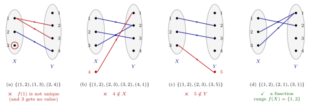
Figure 32: The four candidates drawn out, one panel each, with the offending pairs in red. (a) sends 1 to two places and leaves 3 with no value at all; (b) has a pair starting outside X; (c) has a pair landing outside Y; (d) satisfies all three conditions. Each panel is an arrow diagram: domain left, co-domain right, elements as labelled dots, the two bags named beneath in blue, and each mapping a line carrying a small arrowhead partway along pointing from X to Y.
Drawn out in Figure 32, the three failures are visibly different shapes of mistake: a fan-out from one point of \(X\), a line starting outside \(X\), and a line landing outside \(Y\). Only (d) has exactly one line leaving each of \(1\), \(2\), \(3\), and both endpoints of every line in the right bag.
Q2 from video 24 — co-domain versus range
For a function \(f : X \to Y\) the co-domain is \(Y\) and the range is \(f(X) = \{f(x) : x \in X\}\), which is a subset of \(Y\).
For option (d) above:
\[\text{co-domain} = Y = \{1,2,3,4\} \qquad\qquad \text{range} = \{1,2\} \subseteq Y\]
The distinction in one line: the co-domain is declared when you write \(f : X \to Y\); the range is computed from the pairs. \(3\) and \(4\) are permitted values that this function never takes.
Image and preimage
If \(f : X \to Y\) is any function and \(A\) is any subset of \(X\), then the image of \(A\) is defined by \(f(A) = \{f(x) : x \in A\}\).
If \(f : X \to Y\) is any function and \(B\) is any subset of \(Y\), then the inverse image or preimage of \(B\) is defined by \(f^{-1}(B) = \{x \in X : f(x) \in B\}\).
Both take a set and return a set: \(f(A)\) and \(f^{-1}(B)\) are themselves sets. The emphasis on any matters too: \(f^{-1}(B)\) is defined for every function, invertible or not. It is not an inverse function.
Worked: images and preimages
Let \(X = \{1,2,3\}\) and \(Y = \{1,2,3,4\}\). From Q1 of video 24 above, \(\{(1,2), (2,1), (3,1)\}\) is a function from \(X\) to \(Y\).
So \(f(1) = 2\), \(f(2) = 1\), \(f(3) = 1\).
| Asked for | Working | Answer | |
|---|---|---|---|
| (a) | image of \(\{1\}\) | \(f(1) = 2\) | \(f(\{1\}) = \{2\}\) |
| (b) | image of \(\{2,3\}\) | \(f(2) = 1\), \(f(3) = 1\) | \(f(\{2,3\}) = \{1\}\) |
| (c) | inverse image of \(\{2\}\) | only \(1\) maps to \(2\) | \(f^{-1}(\{2\}) = \{1\}\) |
| (d) | preimage of \(\{1\}\) | both \(2\) and \(3\) map to \(1\) | \(f^{-1}(\{1\}) = \{2,3\}\) |
| (e) | preimage of \(\{3,4\}\) | nothing maps to \(3\) or \(4\) | \(f^{-1}(\{3,4\}) = \emptyset\) |
On an arrow diagram, the images follow the arrows forwards and the preimages follow them backwards. Both diagrams are in functions-on-general-sets.
The three things this set of answers is built to show: an image can shrink (b), a preimage can grow (d), and a preimage can be empty (e) when the set sits outside the range. All three are ordinary, not failures — and every answer is a set, so the braces are not optional. In part (c), write \(\{1\}\), not \(1\).
See also
- proving-set-properties — the reference note for the three methods and the set identities
- functions-on-general-sets — the reference note for the second half
- sets-and-set-notation — the definitions from Lecture 17 that this builds on
- logical-equivalence-laws · proof-techniques · formula-sheet
- 2026-09-03-set-theory-definitions — Lecture 17
- practice-problems — §23 Properties of Sets, with full worked solutions
- practice-problems — §24 Functions Defined on General Sets
Lecture 17 — Set Theory Definitions and Examples
Pre-work: Video 021 (Set Theory Definitions) and Video 022 (More definitions and examples of sets). See sets-and-set-notation for the reference material — every definition below, with the worked examples and the diagrams.
Learning goals
- Understand the distinction between “is an element of” \(x \in A\) and “is a subset of” \(A \subseteq B\).
- Be comfortable with notation for sets including \[x \in A, \quad A \subseteq B, \quad A \subset B, \quad A \cap B, \quad A \cup B, \quad A - B, \quad A^{c}, \quad \mathcal{P}(A), \quad A \times B\]
Element, subset, proper subset
What is the difference between “is a subset of” \(\subseteq\) and “is a proper subset of” \(\subset\)? A four-way comparison settles it:
| \(\subseteq\) | \(\subset\) | |
|---|---|---|
| \(\mathbb{Z}\) against \(\mathbb{R}\) | \(\mathbb{Z} \subseteq \mathbb{R}\) ✓ | \(\mathbb{Z} \subset \mathbb{R}\) ✓ |
| \(\mathbb{Z}\) against itself | \(\mathbb{Z} \subseteq \mathbb{Z}\) ✓ | \(\mathbb{Z} \not\subset \mathbb{Z}\) ✗ |
A set is always a subset of itself, and never a proper subset of itself. That single row is the entire difference — exactly parallel to \(\leq\) against \(<\).
What is the difference between “is a subset of” and “is an element of”? A concrete universe shows it better than a symbol:
Let \(L := \{\text{everyone in the lecture theatre}\}\), and let \(m :=\) me and \(y :=\) you.
Four memberships hold: \(m \in L\), \(y \in L\), \(\{m\} \subseteq L\), \(\{m,y\} \subseteq L\). The two braced objects are sets. A person is an element; a group of people is a subset. One is a person, the other is a collection of people. Just as \(2 \neq \{2\}\) (below), \(m \neq \{m\}\) — a person is not a group containing one person.
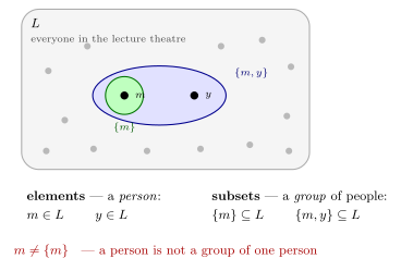
Figure 33: The lecture theatre example drawn out. A person in the room is an element of L; any group of people in the room is a subset of L. The two symbols relate different kinds of thing, which is why m and {m} are not the same object even though the group has exactly one member.
The other people in the room are drawn into Figure 33 for a reason: \(\{m,y\}\) is a subset of \(L\), not the subset. Every group you can pick out of the room is one, and there are a great many of them — how many exactly is the power set fact further down this page.
Why isn’t \(\mathbb{Z} \in \mathbb{Q}\) — aren’t all integers rational numbers? They are, and that is exactly the claim \(\mathbb{Z} \subseteq \mathbb{Q}\). But \(\mathbb{Z} \in \mathbb{Q}\) says \(\mathbb{Z}\) is one of the rational numbers, and \(\mathbb{Z}\) is a set of numbers, not a number. The instinct is right; the symbol is wrong.
Set difference — do the backslash and the minus sign mean the same thing? Yes. \(A - B\) can be written \(A \setminus B\). Purely a matter of which textbook you are reading.
Q2 from the pre-class questions
True or false? \(\;\mathbb{Z} \in \mathbb{Q}\)
False. \(\mathbb{Z}\) is a set of numbers, so it is not an element of \(\mathbb{Q}\); the true statement is \(\mathbb{Z} \subseteq \mathbb{Q}\).
Take care with the distinction between “is an element of” and “is a subset of”.
And one level down: a single element is not the same as the set containing a single element, so \(2 \neq \{2\}\).
Worked: is it an element?
Determine whether each of the following is true or false.
| Statement | Reasoning | ||
|---|---|---|---|
| a) | \(4 \in \{4\}\) | True | \(\{4\}\) contains \(4\) as an element |
| b) | \(4 \in \{\{4\}\}\) | False | \(\{\{4\}\}\) does not contain \(4\) as an element — it does contain \(\{4\}\) as an element |
| c) | \(\{4\} \in \{2,3,4\}\) | False | \(\{2,3,4\}\) does not contain \(\{4\}\) as an element — it does contain \(4\) as an element |
- and (c) are parallel: in each case the set contains something, just not the thing being asked about. \(\{4\} \subseteq \{2,3,4\}\) is true — (c) fails on the symbol, not on the containment.
The reliable technique is to write the set’s elements out as a list and ask whether the left-hand object is literally one of them. For \(\{\{4\}\}\) that list has one entry, the set \(\{4\}\), and \(4\) is not it.
Subsets and proper subsets
A set \(S\) is a subset of a set \(T\), denoted \(S \subseteq T\), if every element that is in \(S\) is also in \(T\). Formally we say \(\forall x\), if \(x \in S\) then \(x \in T\).
A set \(S\) is a proper subset of a set \(T\), denoted \(S \subset T\), if \(S \subseteq T\) and there is an element in \(T\) that is not in \(S\).
Examples: \(\mathbb{Z} \subseteq \mathbb{Q}\) and \(\mathbb{Z} \subseteq \mathbb{Z}\); \(\mathbb{Z} \subset \mathbb{Q}\) but \(\mathbb{Z} \not\subset \mathbb{Z}\).
For sets \(S\) and \(T\), to prove that \(S \subseteq T\), you consider an arbitrary element of \(S\) and show that it is also in \(T\). That is, we suppose \(x \in S\) and prove that \(x \in T\).
Worked: prove one set is a subset of another
(a) Let \(D = \{n \in \mathbb{Z} \mid n \equiv 2 \;(\mathrm{mod}\; 8)\}\) and let \(E\) be the set of even integers. Prove that \(D \subseteq E\).
Writing out both sets first makes the shape of the proof obvious:
\[D = \{\dots, 2, 10, 18, \dots\} \qquad E = \{\dots, 2, 4, 6, 8, \dots\} = \{n \in \mathbb{Z} \mid n \equiv 0 \;(\mathrm{mod}\; 2)\}\]
Rewriting \(E\) as a congruence class is the move that makes the two sets comparable — both are now “\(\equiv\) something”, and the proof is arithmetic.
Proof. Let \(x \in D\). Then \(x \equiv 2 \;(\mathrm{mod}\; 8)\), so \(\exists k \in \mathbb{Z}\) such that \[x = 8k + 2 = 2(4k+1) + 0\] \(\therefore x \equiv 0 \;(\mathrm{mod}\; 2)\), \(\therefore x \in E\). Thus \(D \subseteq E\). \(\blacksquare\)
(b) Is \(D \subset E\)?
Yes. \(4 \in E\) but \(4 \notin D\), so \(D \subseteq E\) is proper. One witness is all a proper containment needs.
When are two sets equal?
For sets \(S\) and \(T\), saying \(S = T\) means \(\forall x\), \(x \in S\) if and only if \(x \in T\).
Recall that \(S \subseteq T\) means \(\forall x\), if \(x \in S\) then \(x \in T\). Since \(p \leftrightarrow q \equiv (p \rightarrow q) \land (q \rightarrow p)\), it follows that \(S = T\) is logically equivalent to \((S \subseteq T) \land (T \subseteq S)\).
So to prove two sets \(S\) and \(T\) are equal you do two separate proofs: suppose \(x \in S\) and prove \(x \in T\) (giving \(S \subseteq T\)), then suppose \(x \in T\) and prove \(x \in S\) (giving \(T \subseteq S\)). Together these show \(S = T\).
This is a consequence, not a convention — it is the biconditional law of logical-equivalence-laws read through the definition of \(\subseteq\).
The empty set
\(\emptyset = \{\;\}\)
Why is \(\emptyset \subseteq A\) for every set \(A\)? Because “\(\forall x\), if \(x \in \emptyset\) then \(x \in A\)” is true for every set \(A\). The hypothesis is never satisfied, so the conditional is vacuously true — the F-hypothesis row of the truth table in conditional-statements is doing all the work.
Take the two halves of the conditional separately: \(x \in \emptyset\) is F — always false, whatever \(x\) is — and \(x \in A\) is F/T, because it could go either way. A conditional with a false hypothesis is true regardless of the conclusion, so the implication holds for every \(x\) and every \(A\).
Do not confuse this with \(\emptyset \in A\). There are some sets that do contain the empty set, but there are lots of sets that do not.
Why is \(A \subseteq A\) for every set \(A\)? Because “\(\forall x\), if \(x \in A\) then \(x \in A\)” is true for every set \(A\) — this time because the conclusion restates the hypothesis.
Lemma. There is only one empty set.
Proof (by contradiction). Suppose that \(\emptyset_1\) and \(\emptyset_2\) are distinct sets each having no elements, so \(\emptyset_1 \neq \emptyset_2\). Since \(\emptyset_1\) has no elements, it is a subset of \(\emptyset_2\), that is, \(\emptyset_1 \subseteq \emptyset_2\). Also since \(\emptyset_2\) has no elements, we have \(\emptyset_2 \subseteq \emptyset_1\). Thus \(\emptyset_1 = \emptyset_2\) by definition of set equality, and we have reached a contradiction. \(\blacksquare\)
Hence \(\emptyset_1 = \emptyset_2 = \emptyset\) — the empty set, which is why it gets a symbol of its own.
Unions and intersections
Let \(A_1 = \{1,2,3\}\), \(A_2 = \{1,2,4\}\) and \(A_3 = \{3,4,5\}\).
\[A_1 \cup A_2 = \{1,2,3,4\} \qquad A_1 \cap A_2 = \{1,2\} \qquad A_1 \cap A_3 = \{3\} \qquad A_2 \cap A_3 = \{4\}\]
\[\bigcup_{i=1}^{3} A_i = A_1 \cup A_2 \cup A_3 = \{1,2,3,4,5\}\]
\[\bigcap_{i=1}^{3} A_i = (A_1 \cap A_2) \cap A_3 = \{1,2\} \cap \{3,4,5\} = \emptyset\]
All three pairwise intersections are non-empty, and the triple intersection is still empty. Pairwise overlap does not propagate to the whole family.
Worked: an infinite union and an infinite intersection
Determine the following sets, recalling the interval notation \([a,b] = \{x \in \mathbb{R} \mid a \leq x \leq b\}\).
\[\bigcup_{i=0}^{\infty} \{i, -i\} = \{0, -0\} \cup \{1,-1\} \cup \{2,-2\} \cup \cdots = \{\dots, -2, -1, 0, 1, 2, \dots\} = \mathbb{Z}\]
\[\bigcap_{i=0}^{\infty} [-i,\, i] = \{0\}\]
For the intersection, the intervals grow with \(i\) — \([0,0] \subseteq [-1,1] \subseteq [-2,2] \subseteq \cdots\) — so the intersection is pinned by the smallest, the \(i=0\) term \([0,0] = \{0\}\). The nested intervals are drawn on a number line in sets-and-set-notation.
The power set
Let \(S = \{1,2,3\}\). Then \(\mathcal{P}(S) = \big\{\emptyset, \{1\}, \{2\}, \{3\}, \{1,2\}, \{1,3\}, \{2,3\}, \{1,2,3\}\big\}\)
The elements of a power set are sets, which resets the \(\in\)/\(\subseteq\) trap one level up:
| \(\{1,2\} \in \mathcal{P}(S)\) | it is one of the eight things listed |
| \(\{1,2\} \not\subseteq \mathcal{P}(S)\) | that would need \(1\) and \(2\) to be elements of \(\mathcal{P}(S)\) |
| \(\big\{\{1,2\}\big\} \subseteq \mathcal{P}(S)\) | its one element, \(\{1,2\}\), is in \(\mathcal{P}(S)\) |
Since \(\emptyset \subseteq A\) for every set \(A\), it follows that \(\emptyset \in \mathcal{P}(A)\) for every set \(A\).
Fact. If \(T\) is a finite set that contains \(n\) elements, then \(|\mathcal{P}(T)| = 2^{n}\).
This fact is important. The finite qualifier is part of it, and the \(2^{n}\) comes from building a subset by making \(n\) independent in-or-out choices.
Worked: element or subset of a power set?
True or false? \(\;\{1, 3, -1\} \subset \mathcal{P}(\mathbb{Z})\)
False, by walking the levels carefully:
\[1, 3, -1 \in \mathbb{Z} \;\;\therefore\; \{1,3,-1\} \subseteq \mathbb{Z} \;\;\therefore\; \{1,3,-1\} \in \mathcal{P}(\mathbb{Z}) \;\;\text{so}\;\; \{1,3,-1\} \not\subset \mathcal{P}(\mathbb{Z})\]
It is an element of the power set, not a subset of it. For it to be a subset, its own elements \(1\), \(3\), \(-1\) would have to be subsets of \(\mathbb{Z}\) — and they are integers, not sets. The statement is off by exactly one level.
Worked: write down each power set
Number the elements while writing them and then check each answer against \(2^n\), which is the cheapest way to catch a dropped brace:
| Power set | Value | Check |
|---|---|---|
| \(\mathcal{P}(\{a\})\) | \(\big\{\emptyset,\; \{a\}\big\}\) | \(|\{a\}| = 1\), so \(2^1 = 2\) ✓ |
| \(\mathcal{P}(\emptyset)\) | \(\big\{\emptyset\big\}\) | \(|\emptyset| = 0\), so \(2^0 = 1\) ✓ |
| \(\mathcal{P}(\mathcal{P}(\emptyset)) = \mathcal{P}(\{\emptyset\})\) | \(\big\{\emptyset,\; \{\emptyset\}\big\}\) | \(|\{\emptyset\}| = 1\), so \(2^1 = 2\) ✓ |
| \(\mathcal{P}(\mathcal{P}(\mathcal{P}(\emptyset))) = \mathcal{P}\big(\{\emptyset, \{\emptyset\}\}\big)\) | \(\big\{\emptyset,\; \{\emptyset\},\; \{\{\emptyset\}\},\; \{\emptyset,\{\emptyset\}\}\big\}\) | \(\big|\{\emptyset,\{\emptyset\}\}\big| = 2\), so \(2^2 = 4\) ✓ |
The line to get right is \(\mathcal{P}(\emptyset) = \{\emptyset\}\): the empty set has exactly one subset — itself — so its power set has one element and is not empty.
Cartesian products
Let \(A_1 = \{1,2\}\), \(A_2 = \{3,4,5\}\) and \(A_3 = \{6\}\).
\[A_1 \times A_2 = \{(1,3), (1,4), (1,5), (2,3), (2,4), (2,5)\}\] \[A_1 \times A_2 \times A_3 = \{(1,3,6), (1,4,6), (1,5,6), (2,3,6), (2,4,6), (2,5,6)\}\]
with \(|A_1 \times A_2| = |A_1| \cdot |A_2| = 2 \times 3 = 6\). The product is drawn as a grid of points in sets-and-set-notation.
Let \(S = \{a,b,c\}\) and \(T = \{c,d\}\).
- \((d,c) \notin S \times T\) since \(d \notin S\) — order matters.
- \((c,d) \in S \times T\) since \(c \in S\) and \(d \in T\).
- \(S \times T\) contains \(3 \times 2 = 6\) elements.
The familiar case is \(\mathbb{R} \times \mathbb{R} = \{(x,y) \mid x \in \mathbb{R} \text{ and } y \in \mathbb{R}\}\), often denoted \(\mathbb{R}^2\).
Two more facts: if \(A = \emptyset\) or \(B = \emptyset\) then \(A \times B = \emptyset\); and for finite sets, \(|A_1 \times A_2 \times \cdots \times A_n| = |A_1| \cdot |A_2| \cdots |A_n|\).
Notation issue to be aware of. \((a,b)\) can be used for an ordered pair. \((a,b)\) can also be used as an interval, representing the real numbers \(x\) where \(a < x < b\). Only context distinguishes them.
Partitions
A finite or infinite collection of non-empty sets \(\{A_1, A_2, A_3, \dots\}\) is a partition of a set \(A\) if and only if \[A = A_1 \cup A_2 \cup A_3 \cup \cdots \qquad\text{and}\qquad A_i \cap A_j = \emptyset \text{ for each } i, j \geq 1,\; i \neq j\]
Examples. A partition of \(\mathbb{Z}\) is given by \(\{E, O\}\) where \(E\) is the even integers and \(O\) the odd integers. Another partition of \(\mathbb{Z}\) is \(\big\{\{0\}, \mathbb{Z}^{+}, \mathbb{Z}^{-}\big\}\) — the same set, partitioned two different ways.
Worked: partitions
(a) Let \(S = \{x \in \mathbb{Z} \mid x \equiv 1 \;(\mathrm{mod}\; 3)\}\), let \(T = \{x \in \mathbb{Z} \mid x \equiv 2 \;(\mathrm{mod}\; 4)\}\), and let \(R = S \cup T\). Is \(\{S,T\}\) a partition of the set \(R\)? Explain why or why not.
No. The covering condition \(R = S \cup T\) holds by definition, but disjointness fails:
\[10 \equiv 1 \;(\mathrm{mod}\; 3) \;\Rightarrow\; 10 \in S \qquad\text{and}\qquad 10 \equiv 2 \;(\mathrm{mod}\; 4) \;\Rightarrow\; 10 \in T\]
So \(10 \in S \cap T\), hence \(S \cap T \neq \emptyset\), and \(\{S,T\}\) is not a partition of \(R\). Stripe the two congruence classes along a number line — pink for \(S\), green for \(T\) — and a tick carrying both colours is a point of \(S \cap T\).
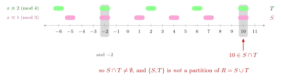
Figure 34: Finding the counterexample: the two congruence classes striped along the integers — S every third integer (pink row), T every fourth (green row) — and read off for a tick that both stripes cover. The grey capsules mark those ticks, which are the overlap.
The grey capsules mark every tick both stripes cover in the range drawn — \(10\) is the witness above, and \(-2\) works equally well. Two witnesses are no better than one here: disjointness is a universal claim, so a single overlap kills it.
(b) State two different partitions of the set \(\mathbb{Z} \times \mathbb{Z}\).
By the sign of the first coordinate: \[R = \{(a,b) \in \mathbb{Z} \times \mathbb{Z} \mid a \geq 0\} \qquad L = \{(a,b) \in \mathbb{Z} \times \mathbb{Z} \mid a < 0\}\] \(\{L, R\}\) is a partition of \(\mathbb{Z} \times \mathbb{Z}\).
By the parity of the second coordinate: \[E = \{(a,b) \in \mathbb{Z} \times \mathbb{Z} \mid b \equiv 0 \;(\mathrm{mod}\; 2)\} \qquad O = \{(a,b) \in \mathbb{Z} \times \mathbb{Z} \mid b \equiv 1 \;(\mathrm{mod}\; 2)\}\] \(\{E, O\}\) is another partition of \(\mathbb{Z} \times \mathbb{Z}\).
Picture \(\mathbb{Z} \times \mathbb{Z}\) as a lattice of dots carrying both partitions at once: a block over the right half of the lattice against a block over the left half for \(\{L, R\}\), and horizontal stripes alternating row by row for the parity split \(\{E, O\}\) — the same “cut the whole thing up and check nothing is covered twice” picture as Figure 34, one dimension up.
The general recipe: any property that every element either has or lacks splits the set into two parts that partition it, provided neither part is empty. Made exact later in the course by equivalence relations.
See also
- sets-and-set-notation — the reference note for all of the above
- proving-set-properties · functions-on-general-sets — where Lecture 18 takes this
- modular-arithmetic — the congruence classes in the subset proof and the partition question
- conditional-statements · logical-equivalence-laws — vacuous truth, and the biconditional behind set equality
- 2026-08-31-solving-recurrence-relations — Lecture 16
- 2026-09-03-set-properties-and-functions — Lecture 18
- practice-problems — §21 Set Theory Definitions, with full worked solutions
- practice-problems — §22 More Definitions and Examples of Sets
Week 7
Lecture 19 — Functions: One-to-One, Onto, Inverse
Pre-work: Video 025 (One-to-one, onto, and inverse functions). The reference notes are one-to-one-and-onto-functions for the two properties and their proof templates, and inverse-functions for bijections, inverses, and the two meanings of \(f^{-1}\); the definition of a function itself is in functions-on-general-sets.
Date. The published schedule puts Lecture 19 on Tuesday 08/09, but the course has been running one lecture ahead of it since Lecture 15 (see the note under math1061), which makes this the Monday 07/09 lecture and 2026-09-08-composition-of-functions the Tuesday. Confirm against Blackboard.
Learning goals
- Understanding what a function is, and associated concepts and definitions.
- How to show functions are one-to-one (injective), onto (surjective), bijective.
The picture throughout is \(f : X \to Y\) as two ellipses: \(X\) is the domain, \(Y\) is the co-domain, and an arrow \(f\) takes \(x\) in \(X\) to \(f(x)\) in \(Y\). An arrow back from \(f(x)\) to \(x\) would be \(f^{-1}\). The whole topic is when that arrow back is allowed to exist.
The co-domain is part of the function
Defining the co-domain differently can make a function onto.
\[f : \mathbb{R} \to \mathbb{R}, \; f(x) = x^2 \text{ is not onto} \qquad\qquad g : \mathbb{R} \to \mathbb{R}^{\geq 0}, \; g(x) = x^2 \text{ is onto.}\]
The parabola never reaches the negative half of the \(y\)-axis, so as a function to \(\mathbb{R}\) those values are missed. Same rule, same domain, same pairs — only the declared co-domain differs, and onto is a statement about the declared co-domain (functions-on-general-sets). Shrink the co-domain to the range and every function becomes onto; that is what \(g\) does.
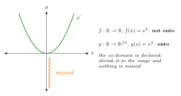
Figure 35: The parabola \(x^2\), with the negative \(y\)-axis marked missed in orange. As a function to \(\mathbb{R}\) every negative value is missed, so \(f\) is not onto; declare the co-domain to be \(\mathbb{R}^{\geq 0}\) and nothing is missed, so \(g\) is onto. Same rule, same graph.
\(f\) and \(g\) are different functions under the course’s definition, even though they contain exactly the same ordered pairs, because a function is written \(f : X \to Y\) and \(Y\) is part of the declaration.
The inverse function of \(f\) does not have the same domain and co-domain as \(f\).
\[f : X \to Y \quad\text{then}\quad f^{-1} : Y \to X.\]
They are swapped. The inverse goes the other way, so its domain is \(f\)’s co-domain and its co-domain is \(f\)’s domain.
Definition of a function
\(f : X \to Y\) is \(f \subseteq X \times Y\) such that for each \(x \in X\), there is a unique \(y \in Y\) such that \((x,y) \in f\).
The unique \(y\) is written \(f(x) = y\). There are three things to check: \(x \in X\), \(y \in Y\), and \(\forall x \in X\), \(f(x)\) is unique. A fan-out fails the definition: one dot in \(X\) with three arrows leaving it is not a function.
Which of the following are functions? The verdicts, each with the reason:
| Verdict | Why | ||
|---|---|---|---|
| 1 | \(f : \mathbb{R} \to \mathbb{R}\), \(f(x) = x^2\) | Function | |
| 2 | \(f : \mathbb{Z}^{+} \to \mathbb{Z}^{+}\), \(f(n) = n!\) | Function | \(n! = n(n-1)\cdots 3 \cdot 2 \cdot 1 \in \mathbb{Z}^{+}\) |
| 3 | \(f : \mathbb{Z}^{+} \to \mathbb{Z}^{+}\), \(f(n) = \dfrac{(n+1)(n+3)}{3}\) | Not a function | \(\dfrac{(n+1)(n+3)}{3}\) might not be in the co-domain \(\mathbb{Z}^{+}\) — e.g. \(n = 1\) gives \(\frac{8}{3}\) |
| 4 | \(f : \mathbb{R} \to \mathbb{R}\), \(f(x) = 1\) | Function | \(\{(x,1) : x \in \mathbb{R}\}\) — constant is fine |
| 5 | \(f : \mathbb{Q} \to \mathbb{Z}\), \(f\!\left(\frac{m}{n}\right) = m\) for all \(m, n \in \mathbb{Z}\), \(n \neq 0\) | Not a function | \(f\!\left(\frac{1}{2}\right) = 1\) but \(f\!\left(\frac{2}{4}\right) = 2\), and \(\frac{1}{2} = \frac{2}{4}\) — one input, two values |
| 6 | \(f : \mathbb{R} \to \mathbb{R}\), \(f = \{(x,y) : 3y + 7 = x\}\) | Function | \(y = \dfrac{x - 7}{3}\) |
| 7 | \(f : \mathbb{R} \to \mathbb{R}\), \(f = \{(x,y) : y^2 = x\}\) | Not a function | e.g. \((4,2), (4,-2) \in f\) — a sideways parabola, which a vertical line meets twice |
| 8 | \(f : \mathbb{R} \to \mathbb{R}\), \(f = \{(x,y) : x = \lvert y \rvert\}\) | Not a function | e.g. \((1,1), (1,-1) \in f\) — a sideways V, same test |
Each failure breaks one of two clauses. 3 lands outside the co-domain (the \(y \in Y\) clause). 5, 7 and 8 give one input two values (unique) — and 5 is the subtle one, because it looks like a rule until you remember that a rational number has many names. A rule that depends on how the input is written rather than on what the input is is not well defined, which is the standard name for exactly this failure.
7 and 8 are the vertical line test from functions-on-general-sets, run on curves that are not graphs of \(y\) against \(x\) — the two red curves in Figure 36.
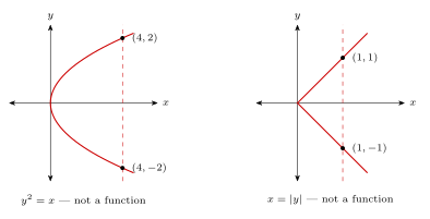
Figure 36: Items 7 and 8. \(y^2 = x\) is a parabola opening to the right; \(x = |y|\) is a V opening to the right. The dashed vertical line meets each curve twice — at \((4,2)\) and \((4,-2)\), at \((1,1)\) and \((1,-1)\) — and each pair of points is the witness that the set of pairs is not a function.
Injective and surjective
Let \(f\) be a function, \(f : X \to Y\).
Injective function (one-to-one function): \(\forall x_1, x_2 \in X\), if \(f(x_1) = f(x_2)\) then \(x_1 = x_2\).
Surjective function (onto function): \(\forall y \in Y\), \(\exists x \in X\) such that \(f(x) = y\).
One-to-one is also written one-one. The two failures are drawn in Figure 37:
- not one-to-one — \(x_1\) and \(x_2\) in \(X\), both arrows landing on the same dot \(f(x_1) = f(x_2)\) in \(Y\).
- not onto — the whole domain pours into the range, an inner ellipse of \(Y\), and one dot in \(Y\) lies outside it: range \(\subset\) co-domain.
Figure 37: The two ways a function can fall short. Left: not one-to-one, two different inputs sharing one output; the blue rings mark the two sources and the one target. Right: not onto, the whole domain funnelled into a range (hatched in blue) that is a proper subset of the co-domain; the dot outside the hatching is a y that no x reaches. Domain on the left, co-domain on the right, names above.
Two examples on the plane, graphed in Figure 38:
\[f : \mathbb{R} \to \mathbb{R}, \; f(x) = x^3 - x \text{ is surjective but not injective.}\] \[f : \mathbb{R} \to \mathbb{R}, \; f(x) = 2^x \text{ is injective but not surjective.}\]
Figure 38: The two graphed examples. The cubic \(x^3 - x\) takes every real value, so it is onto, but takes the value 0 three times (and every value in its middle band three times), so it is not one-to-one; the dashed horizontal line is the horizontal line test. The exponential \(2^x\) never repeats a value, so it is one-to-one, but never reaches 0 or anything below it, so as a function to \(\mathbb{R}\) it is not onto.
The two properties are independent: Figure 38 has one of each, and the constant function \(f(x) = 1\) above has neither.
How to show it
There are four templates, two for showing a property and two for showing its failure:
| To show \(f : X \to Y\) is … | Do |
|---|---|
| one-to-one | suppose that \(f(x_1) = f(x_2)\) and show that \(x_1 = x_2\) |
| not one-to-one | find elements \(x_1, x_2 \in X\) such that \(f(x_1) = f(x_2)\) and \(x_1 \neq x_2\) |
| onto | suppose that \(y \in Y\) and find an \(x \in X\) such that \(f(x) = y\) |
| not onto | find an element \(y \in Y\) such that for all \(x \in X\), \(f(x) \neq y\) |
The pattern is the same one as for sets (2026-09-03-set-properties-and-functions): a universal claim (is one-to-one, is onto) needs a general argument from an arbitrary element, and its negation needs one witness. Which is why the two “not” rows are so much shorter to do — and why a proof of one-to-one that checks a few values proves nothing.
Worked: a bijection onto the odd integers
Consider the function \(g : \mathbb{Z} \to \mathbb{Z}^{\text{odd}}\) defined by \(g(x) = 2x + 3\). (a) Is \(g\) an injective function? (b) Is \(g\) a surjective function?
Yes and Yes. That is the intuition; the proofs follow.
(a) Proof. Let \(x_1, x_2 \in \mathbb{Z}\) such that \(g(x_1) = g(x_2)\). Hence \[2x_1 + 3 = 2x_2 + 3, \qquad 2x_1 = 2x_2, \qquad x_1 = x_2.\] \(\therefore g\) is one-to-one. \(\square\)
(b) Proof. Let \(y \in \mathbb{Z}^{\text{odd}}\). Take \(x = \dfrac{y - 3}{2}\). Since \(y\) is odd, \(y - 3\) is even, so \(\dfrac{y-3}{2} \in \mathbb{Z}\). And \[g\!\left(\frac{y-3}{2}\right) = 2\left(\frac{y-3}{2}\right) + 3 = (y - 3) + 3 = y,\] so \(\forall y \in \mathbb{Z}^{\text{odd}}\), \(\exists x \in \mathbb{Z}\) s.t. \(g(x) = y\). \(\therefore g\) onto. \(\square\)
The thinking behind (b) is not part of the proof: want to find \(x \in \mathbb{Z}\) such that \(g(x) = y\); \(2x + 3 = y\); \(x = \frac{y-3}{2}\). That is scratch work — solving for \(x\) backwards — and the proof then runs it forwards: name the candidate, check it is in the domain, check \(g\) sends it to \(y\). The “check it is in the domain” line is the one that gets skipped: it is exactly where the oddness of \(y\) is used, and without it the argument would “prove” \(g : \mathbb{Z} \to \mathbb{Z}\) onto, which is false.
Worked: a function on pairs
Define a function \(f : \mathbb{R} \times \mathbb{R} \to \mathbb{R} \times \mathbb{R}\) by \(f((x,y)) = (y + 1, 2x)\). For example, \(f((0,0)) = (1,0)\) and \(f((-2,3)) = (4,-4)\).
In the example \(f((0,0)) = (1,0)\), the input’s second entry \(y\) feeds the first entry of the output, and the input’s first entry \(x\) feeds the second. The inputs and outputs are pairs, and the coordinates cross over.
(a) Prove that \(f\) is one-to-one. Suppose \((x_1,y_1), (x_2,y_2) \in \mathbb{R} \times \mathbb{R}\) and \(f((x_1,y_1)) = f((x_2,y_2))\). Then \((y_1 + 1, 2x_1) = (y_2 + 1, 2x_2)\). So \[y_1 + 1 = y_2 + 1 \;\text{ and }\; 2x_1 = 2x_2, \qquad y_1 = y_2 \;\text{ and }\; x_1 = x_2.\] So \((x_1,y_1) = (x_2,y_2)\). \(\square\)
The first entries give one equation, the second entries give another, and the and between them matters. Two ordered pairs are equal exactly when both coordinates agree, so one equation of pairs is two equations of numbers, and both are needed.
(b) Prove that \(f\) is onto. Suppose \((a,b) \in \mathbb{R} \times \mathbb{R}\) (co-domain). Take \(\left(\frac{b}{2}, a - 1\right) \in \mathbb{R} \times \mathbb{R}\) (domain), and \[f\!\left(\left(\tfrac{b}{2}, a - 1\right)\right) = \left((a-1) + 1, \; 2\left(\tfrac{b}{2}\right)\right) = (a,b).\] \(\therefore f\) is onto. \(\square\)
The scratch work behind the candidate: want \(f((x,y)) = (a,b)\); \((y+1, 2x) = (a,b)\); \(y + 1 = a\) and \(2x = b\); \(y = a - 1\), \(x = \frac{b}{2}\). Same method as for \(g\) above, one coordinate at a time. Here the domain check is trivial — \(\frac{b}{2}\) and \(a - 1\) are real whenever \(a\) and \(b\) are — which is why it is written as a bare (domain) label rather than argued.
This function returns in 2026-09-08-composition-of-functions, where its inverse is computed from exactly this working.
Inverse functions
A function that is both one-to-one and onto is said to be a bijection.
A bijection \(f : X \to Y\) has an inverse function \(f^{-1} : Y \to X\).
\(f : X \to Y\) takes \(x_1 \mapsto f(x_1)\) and \(x_2 \mapsto f(x_2)\), and \(f^{-1} : Y \to X\) runs the other way.
The two failure cases are drawn in Figure 39:
- not one-to-one \(\Rightarrow\) no inverse (green) — two dots of \(X\) going to one dot of \(Y\); the orange arrow back from that dot is marked ?, because it would have to go to two places.
- not onto \(\Rightarrow\) no inverse (purple) — a dot of \(Y\) outside the range; the arrow back from it is marked ?, because there is nowhere for it to go.
Figure 39: Why an inverse needs both properties. Left (green): if \(f\) is not one-to-one, the arrow back from a shared output has two candidates and cannot be a function. Right (purple): if \(f\) is not onto, the arrow back from an unreached \(y\) has no candidate at all. An inverse function has to send every \(y \in Y\) to exactly one \(x\) — onto supplies the every, one-to-one supplies the exactly one.
Q2 from the pre-class questions
Let \(f : X \to Y\) be a bijective function. Which one of the following is true?
| Why | |||
|---|---|---|---|
| a) | The inverse function of \(f\) does not exist. | ✗ | a bijection is exactly the case where the inverse does exist |
| b) | For all \(y \in Y\), \(f^{-1}(y) = x\) where \(x\) is the unique element in \(X\) such that \(f(x) = y\). | ✓ | \(x\) exists since \(f\) is onto; it is unique since \(f\) is one-to-one |
| c) | \(f^{-1}\) is a function from \(X\) to \(Y\). | ✗ | the inverse runs \(Y \to X\) |
| d) | \(X\) and \(Y\) are finite. | ✗ | nothing about bijections needs finiteness — \(g(x) = 2x + 3\) above is a bijection between infinite sets |
Option b) is the definition of \(f^{-1}\), and its two reasons are the whole topic in one sentence: onto gives existence, one-to-one gives uniqueness.
The notation \(f^{-1}\) is used in two different ways
This distinction is important.
1. If \(f : X \to Y\) is any function and \(A\) is any subset of \(Y\), then the inverse image or preimage \(f^{-1}(A)\) of \(A\) is defined by \[f^{-1}(A) = \{x \in X : f(x) \in A\}.\] Notice that the preimage function \(f^{-1}\) is a function \(f^{-1} : \mathcal{P}(Y) \to \mathcal{P}(X)\).
2. If \(f : X \to Y\) is any bijective function then the inverse function of \(f\) is the function \(f^{-1} : Y \to X\) where for all \(y \in Y\) \[f^{-1}(y) = x \text{ where } x \text{ is the unique } x \in X \text{ such that } f(x) = y.\] Notice that the inverse function \(f^{-1}\) is a function \(f^{-1} : Y \to X\).
Both are drawn in inverse-functions. In the first, \(f\) is many-to-one and a blob \(f^{-1}(A)\) in \(X\) collects everything that lands in the blob \(A\) in \(Y\). In the second, \(f\) is bijective (one-to-one and onto) and a single arrow \(f^{-1}\) runs back from \(y\) to \(x\).
The difference is in what goes in and what comes out:
| Input | Output | Exists for | |
|---|---|---|---|
| preimage \(f^{-1}(A)\) | a subset of \(Y\) | a subset of \(X\) | every function |
| inverse function \(f^{-1}(y)\) | an element of \(Y\) | an element of \(X\) | bijections only |
Preimages are defined in functions-on-general-sets and nothing about them has changed; what is new is that the same symbol now also has a second, much more restricted meaning, and the braces are what tell you which one is meant.
Worked: preimage or inverse function?
Let \(f : \{1,2,3,4\} \to \{a,b,c\}\) be the function \(f = \{(1,a), (2,a), (3,b), (4,b)\}\). For each of the following statements about the function \(f\), decide whether the statement is true or false.
The arrow diagram is Figure 148: \(1, 2 \to a\); \(3, 4 \to b\); \(c\) untouched.
| Statement | Why | ||
|---|---|---|---|
| (1) | The inverse function \(f^{-1}\) of \(f\) does not exist. | T | since \(f\) is not a bijection |
| (2) | The preimage of the set \(\{a\}\) is \(f^{-1}(\{a\}) = \{1,2\}\). | T | \(\{a\}\) is a subset of the co-domain; 1 and 2 map to \(a\) (no others map to \(a\)) |
| (3) | \(f^{-1}(a)\) is not defined. | T | \(a\) is an element of the co-domain; here the \(f^{-1}\) notation represents the inverse function, which is not defined for this \(f\) |
| (4) | \(f^{-1}(\{c\}) = \emptyset\). | T | \(\{c\}\) is a subset of the co-domain; the pre-image of \(\{c\}\) is \(\emptyset\) since no element maps to \(c\) |
Figure 40: The function \(f\) as an arrow diagram. It is neither one-to-one (1 and 2 share \(a\), 3 and 4 share \(b\)) nor onto (\(c\) is never reached), so there is no inverse function and \(f^{-1}(a)\) means nothing. But preimages exist for every function: \(f^{-1}({a})\) collects 1 and 2 (green), and \(f^{-1}({c})\) collects nothing (purple, empty).
All four are true, and (2)–(4) are the same lesson three times: read the braces. \(\{a\}\) and \(\{c\}\) are sets, so \(f^{-1}\) means preimage and the answer is a set — possibly empty, which is an answer and not an error. \(a\) alone is an element, so \(f^{-1}\) would have to mean the inverse function, which this \(f\) does not have.
See also
- one-to-one-and-onto-functions — the two definitions, the four proof templates, and more worked examples
- inverse-functions — bijections, the inverse function, and the two meanings of \(f^{-1}\)
- functions-on-general-sets — the definition of a function, co-domain versus range, image and preimage
- 2026-09-03-set-properties-and-functions — Lecture 18 · 2026-09-08-composition-of-functions — Lecture 20
- practice-problems — §25, with full worked solutions
Lecture 20 — Composition of Functions
Pre-work: Video 026 (Composition of functions). The reference note is composition-of-functions; the properties it builds on are in one-to-one-and-onto-functions and inverse-functions. The order here: the one-to-one and onto templates again, two worked examples on inverses, then the composition results.
Date. On the schedule this is the Thursday 10/09 lecture; on the one-ahead reading explained under math1061 it is Tuesday 08/09.
Learning goals
- Review definitions of injective and surjective functions.
- Investigate conditions for a composition of functions to be one-to-one, onto.
The picture to keep in mind has three sets \(X\), \(Y\), \(Z\). \(f\) sends \(x \mapsto f(x)\), a hop \(X \to Y\). \(g\) sends \(f(x) \mapsto g(f(x))\), a hop \(Y \to Z\). \(g \circ f\) goes from \(x\) straight to \(g(f(x))\).
Worked: is \(f \circ g\) also a bijection?
If \(f : X \to Y\) and \(g : Y \to Z\) are both bijective functions, then the composition \(g \circ f : X \to Z\) is also a bijection. In this case, is \(f \circ g\) also a bijection?
For \(f \circ g\) to be defined, we need \(X = Z\). With that, yes, \(f \circ g\) is a bijection.
\(f \circ g\) means \(g\) first, then \(f\): \(Y \xrightarrow{\;g\;} Z \xrightarrow{\;f\;} Y\), with \(Z = X\). So \(g\)’s outputs — elements of \(Z\) — have to be things \(f\) accepts — elements of \(X\). Unless \(Z = X\) the expression is not meaningless-but-false; it is simply undefined. Composition is not commutative, and most of the time the other order does not even exist.
The one-to-one and onto templates
The four templates were first met in 2026-09-07-functions-one-to-one-onto-inverse. Going backwards along \(f\) shows the two ways an inverse fails. When \(f\) is not one-to-one, the shared value \(f(x_1) = f(x_2)\) leads back to two sources. When \(f\) is not onto, the unreached element of \(Y\) has nothing to lead back to.
Injective (one-to-one): to show, suppose \(f(x_1) = f(x_2)\) and show \(x_1 = x_2\); to show not, find \(x_1 \neq x_2\) with \(f(x_1) = f(x_2)\).
Surjective (onto): to show, suppose \(y \in Y\) and find \(x \in X\) with \(f(x) = y\); to show not, find \(y \in Y\) with \(f(x) \neq y\) for all \(x\).
Bijective: both. A bijection \(f : X \to Y\) has an inverse function \(f^{-1} : Y \to X\), with \(f^{-1}(y) = x\) where \(x\) is the unique element in \(X\) such that \(f(x) = y\). The converse holds too, which makes it an equivalence:
\[f \text{ has an inverse} \iff f \text{ is a bijection.}\]
Worked: the largest prime divisor
Consider the function \(f : \mathbb{Z} - \{-1, 0, 1\} \to \mathbb{Z}^{>1}\) defined by \(f(x) = p\), where \(p\) is the largest prime divisor of \(x\).
Some values first, to see what the function does: \(f(2) = 2\), \(f(10) = 5\), \(f(-6) = 3\). Removing \(-1\), \(0\), \(1\) from the domain is what makes it a function at all: \(\pm 1\) have no prime divisor, and \(0\) is divisible by every prime, so it has no largest one.
(a) Is \(f\) an injection? \(f(10) = 5\), \(f(15) = 5\) and \(10 \neq 15\). Not injective.
(b) Is \(f\) a surjection? No. \(4 \in \mathbb{Z}^{>1}\) but \(4 = 2 \cdot 2\) is not prime, so \(\nexists\, x \in \mathbb{Z} - \{-1,0,1\}\) s.t. \(f(x) = 4\).
(c) Is \(f\) a bijection? If it exists, determine \(f^{-1}\). No. \(f^{-1}\) does not exist (d.n.e.).
The two disproofs are both single witnesses, as the templates say they should be. For (b) the witness is any composite number — the range of \(f\) is the primes, and \(\mathbb{Z}^{>1}\) has far more in it.
Worked: reading \(f^{-1}\) off the onto proof
The function \(f : \mathbb{R} \times \mathbb{R} \to \mathbb{R} \times \mathbb{R}\) defined by \(f((x,y)) = (y + 1, 2x)\) is both one-to-one and onto (proved in 2026-09-07-functions-one-to-one-onto-inverse). Determine \(f^{-1}\).
The onto half of that proof is the part to use. The candidate it named was \(\left(\frac{b}{2}, a - 1\right)\). That candidate is the inverse:
\[f^{-1} : \mathbb{R} \times \mathbb{R} \to \mathbb{R} \times \mathbb{R}, \qquad f^{-1}((a,b)) = \left(\tfrac{b}{2}, \; a - 1\right),\]
or, renaming the variables to the usual ones, \(f^{-1}((x,y)) = \left(\frac{y}{2}, \; x - 1\right)\).
Sense check: \(f \circ f^{-1}((x,y)) = (x,y)\) and \(f^{-1} \circ f((x,y)) = (x,y)\). Run one of them: \[f\!\left(f^{-1}((x,y))\right) = f\!\left(\left(\tfrac{y}{2}, x - 1\right)\right) = \left((x - 1) + 1, \; 2 \cdot \tfrac{y}{2}\right) = (x, y). \;\checkmark\]
The method is the one to remember: the onto proof already computes the inverse. Showing \(f\) is onto means, for an arbitrary \((a,b)\), finding the \((x,y)\) that maps to it — and the formula for that \((x,y)\) in terms of \((a,b)\) is \(f^{-1}\). The formula is a function in its own right; one-to-one is what makes it the inverse — it guarantees the candidate is the only preimage, so that \(f^{-1} \circ f\) is the identity as well as \(f \circ f^{-1}\). There is no separate “find the inverse” technique.
Composition of functions
Let \(f : X \to Y\) and \(g : Y \to Z\) be functions. Then the composition of \(f\) and \(g\) is the function \(g \circ f : X \to Z\) defined by the rule \[(g \circ f)(x) = g(f(x)) \quad\text{for all } x \in X.\]
Read \(g \circ f\) right to left: \(f\) acts first, then \(g\). The name is in the “wrong” order because the formula \(g(f(x))\) is.
Two properties pass from \(f\) and \(g\) to the composite:
- \(f\) and \(g\) both onto \(\;\rightarrow\; g \circ f\) is onto
- \(f\) and \(g\) both one-to-one \(\;\rightarrow\; g \circ f\) is one-to-one
\(g \circ f\) has domain equal to the domain of \(f\), which is \(X\), and co-domain equal to the co-domain of \(g\), which is \(Z\). The middle set \(Y\) disappears from the type of the composite.
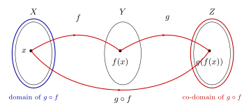
Figure 41: The composition \(g \circ f\). \(X\) (blue outline) is the domain of \(g \circ f\) because it is the domain of \(f\), and \(Z\) (red outline) is its co-domain because it is the co-domain of \(g\). The middle set \(Y\) is where \(f\) lands and \(g\) starts, and it does not appear in \(g \circ f : X \to Z\) at all.
The converse: from \(g \circ f\) back to \(f\) and \(g\)
Those two facts go one way. The converse asks which of the two ingredients must have a property when the composite has it.
For all functions \(f : X \to Y\) and \(g : Y \to Z\):
- Find a counterexample that disproves: if \(g \circ f\) is onto, then \(f\) is onto.
- Prove that: if \(g \circ f\) is onto, then \(g\) is onto. (Proof by contraposition.)
- Prove that: if \(g \circ f\) is one-to-one, then \(f\) is one-to-one.
- Find a counterexample that disproves: if \(g \circ f\) is one-to-one, then \(g\) is one-to-one.
Statements (1) and (2) have the same hypothesis, if \(g \circ f\) is onto, and two different conclusions, one false and one true. The four results, in one table:
| If \(g \circ f\) is … | then \(f\) is … | then \(g\) is … |
|---|---|---|
| onto | not necessarily — (1) | onto — (2) |
| one-to-one | one-to-one — (3) | not necessarily — (4) |
The property propagates to the function on the same side as the property’s quantifier: onto is about reaching everything in \(Z\), and it is \(g\) that lands in \(Z\); one-to-one is about not merging anything from \(X\), and it is \(f\) that leaves \(X\).
(1) Counterexample
Let \(X = \{a,b\}\), \(Y = \{0,1,2\}\), \(Z = \{v,w\}\). Define \(f : X \to Y\) and \(g : Y \to Z\) by \[f = \{(a,0), (b,1)\}, \qquad g = \{(0,v), (1,w), (2,w)\}.\] \(f\) is not onto (since \(2 \in Y\) but \(\nexists\, x \in X\) s.t. \(f(x) = 2\)). Then \(g \circ f = \{(a,v), (b,w)\}\), which is onto (since \(v \in Z\) and \(g \circ f(a) = v\); \(w \in Z\) and \(g \circ f(b) = w\)).
Figure 42 draws it, with yellow highlights on the elements that matter.
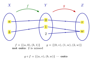
Figure 42: The counterexample for (1). \(f\) misses 2, so \(f\) is not onto; but \(g\) sends 1 and 2 to the same place, so the miss never shows: \(g \circ f\) still reaches both \(v\) and \(w\). The yellow highlights are on \(a\), \(b\), \(0\), \(1\), \(v\), \(w\) — every element the composite actually touches — and 2 is left plain. The function \(g\) has covered for \(f\)’s gap.
(2) Proof
We prove the contrapositive statement: \(\forall\) functions \(f : X \to Y\) and \(g : Y \to Z\), if \(g\) is not onto then \(g \circ f\) is not onto.
Let \(f : X \to Y\) and \(g : Y \to Z\) be functions and suppose \(g\) is not onto. Then \(\exists\, z \in Z\) such that \(z\) is not in the range of \(g\). Thus \(\nexists\, x \in X\) with \(g(f(x)) = z\), i.e. \(z\) is not in the range of \(g \circ f\).
(why? Since if there were such an \(x \in X\) we could take \(y = f(x)\) to give \(g(y) = z\) \((\Rightarrow\Leftarrow)\))
\(\therefore g \circ f\) is not onto. \(\square\)
The contrapositive is the natural shape because not onto hands you a concrete object — a missed \(z\) — to work with, where onto would hand you only a hypothesis about every \(z\). The bracketed why? is a tiny proof by contradiction nested inside: anything \(g \circ f\) reaches, \(g\) reaches too (via \(y = f(x)\)), so a \(z\) that \(g\) misses, \(g \circ f\) misses. Figure 43 shows it: the range of \(g\) is hatched at the top of \(Z\), where \(g\)’s arrow lands, and the lone dot \(z\) sits below it, outside the hatching.
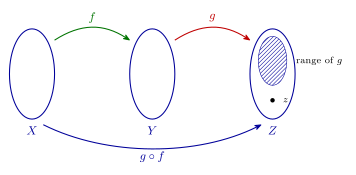
Figure 43: The proof of (2) as a picture. \(g\)’s arrow lands in the hatched region, its range; the dot \(z\) sits outside it. Whatever \(f\) does, \(g \circ f\) can only land where \(g\) lands, so \(z\) is outside the range of \(g \circ f\) too. The mirror of the picture for (3): there a collision in \(f\) survives \(g\), here a gap in \(g\) survives \(f\).
(3) Proof
We prove the contrapositive: \(\forall\) functions \(f : X \to Y\) and \(g : Y \to Z\), if \(f\) is not one-to-one then \(g \circ f\) is not one-to-one.
Let \(f : X \to Y\) and \(g : Y \to Z\) be functions and suppose \(f\) is not one-to-one. Then \(\exists\, x_1, x_2 \in X\) such that \(x_1 \neq x_2\) and \(f(x_1) = f(x_2)\). Hence \[g \circ f(x_1) = g(f(x_1)) = g(f(x_2)) = g \circ f(x_2),\] and since \(x_1 \neq x_2\), \(g \circ f\) is not one-to-one. \(\square\)
Same shape as (2), mirrored. Not one-to-one hands you a concrete collision \(x_1 \neq x_2\), and the collision survives applying \(g\) because \(g\) is a function: equal inputs give equal outputs. Figure 44 shows the collision.
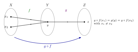
Figure 44: The proof of (3) as a picture. Two different \(x\)’s collide under \(f\) at one \(y\); \(g\) then has only one \(y\) to act on, so it can only send them both to the same \(z\). A collision in \(f\) is a collision in \(g \circ f\), whatever \(g\) does.
(4) Counterexample
Let \(X = \{a,b\}\), \(Y = \{1,2,3\}\), \(Z = \{u,v\}\). Define \(f : X \to Y\) and \(g : Y \to Z\) by \[f = \{(a,1), (b,2)\}, \qquad g = \{(1,u), (2,v), (3,v)\}.\] Then \(g\) is not one-to-one (since \(2 \neq 3\) and \(g(2) = g(3)\)). Now \(g \circ f : X \to Z\) is given by \(\{(a,u), (b,v)\}\), which is one-to-one.
Figure 45: The counterexample for (4). \(g\) merges 2 and 3, so \(g\) is not one-to-one — but \(f\) never sends anything to 3, so the merge is never exercised: \(g \circ f\) sends \(a\) and \(b\) to different places.
The two counterexamples are mirror images and were built the same way. In (1), \(f\) has a gap and \(g\) merges so the gap does not reach \(Z\). In (4), \(g\) merges and \(f\) has a gap so the merge is never fed. In both, the middle set \(Y\) has one more element than it needs — the element that \(f\) misses — and that spare element is where the bad behaviour is parked. Small sets, one thing wrong, the wrong thing hidden: that is how to build a counterexample to order.
See also
- composition-of-functions — the definition, the four converse results as theorems, and how to build the counterexamples
- one-to-one-and-onto-functions · inverse-functions — the properties being composed
- proof-techniques — contraposition, which both proofs use
- 2026-09-07-functions-one-to-one-onto-inverse — Lecture 19
- practice-problems — §26, with full worked solutions
Week 8
Lecture 21 — Cardinalities
Pre-work: Video 027 (Cardinalities). The reference notes are [cardinality] for what “the same size” means and how to prove it, and countable-and-uncountable-sets for the listing arguments that start here and finish in 2026-09-15-countable-and-uncountable-sets. Every tool used is a bijection, so one-to-one-and-onto-functions is the prerequisite.
Learning goals
- Understand cardinalities of finite and infinite sets.
- Learn how to prove properties concerning cardinalities of sets.
The picture to keep in mind is two columns of dots, each dot joined to a partner in the other column, both columns going on without end. It is a pairing that never runs out, and that is the whole idea.
Worked: why is \(|\mathbb{Z}| = |\mathbb{Z}^{+}| = |\mathbb{Q}|\)?
If cardinality is a measure of how large a set is, then why is \(|\mathbb{Z}| = |\mathbb{Z}^{+}| = |\mathbb{Q}|\), when clearly \(|\mathbb{Q}| > |\mathbb{Z}| > |\mathbb{Z}^{+}|\)?
\(|\mathbb{Q}| > |\mathbb{Z}| > |\mathbb{Z}^{+}|\) is false. The clearly is the mistake. Put \(1, 2, 3, 4, 5\) over \(\{a, b, c, d, e\}\) and join each number to one letter. That is what counting a finite set is: pairing its elements off with \(1, 2, \dots, n\). Cardinality keeps the pairing and drops the requirement that it stop.
The “clearly” comes from containment. \(\mathbb{Z}^{+} \subset \mathbb{Z} \subset \mathbb{Q}\), each a proper subset of the next, and for finite sets a proper subset is always smaller. For infinite sets that inference fails, and the proofs below show it. Every example below is infinite.
How do we measure the size of infinite sets?
\(\mathbb{Z}^{+}\) : the positive integers \(1, 2, 3, \dots\)
\(2\mathbb{Z}^{+}\) : the even positive integers \(2, 4, 6, \dots\)
There are two ways to set the two sets side by side. The first is as a subset: \(2\mathbb{Z}^{+} \subset \mathbb{Z}^{+}\), the even entries in the row \(1, 2, 3, \dots\). That is not how to think of it. The second is as a pairing: \(\mathbb{Z}^{+}\) sits over \(2\mathbb{Z}^{+}\), with each \(n\) joined to \(2n\).
To measure the size of infinite sets, think with functions:
\[|2\mathbb{Z}^{+}| = |\mathbb{Z}^{+}|, \qquad f : \mathbb{Z}^{+} \to 2\mathbb{Z}^{+},\; f(x) = 2x,\; f \text{ is a bijection.}\]
Figure 46: Two ways of setting the even positive integers beside the positive integers. Top: as a subset, \(2\mathbb{Z}^{+}\) is every second entry, which makes it look like half of \(\mathbb{Z}^{+}\). Bottom: as a pairing, \(n \leftrightarrow 2n\) matches every positive integer with exactly one even number and every even number with exactly one positive integer, with nothing left over on either side. Cardinality is defined by the pairing, so \(|2\mathbb{Z}^{+}| = |\mathbb{Z}^{+}|\) even though \(2\mathbb{Z}^{+}\) is a proper subset.
Both halves of “bijection” are quick. One-to-one: \(2x_1 = 2x_2\) gives \(x_1 = x_2\). Onto: an even positive integer \(y\) is \(2k\) for some \(k \in \mathbb{Z}^{+}\), and \(f(k) = y\).
Finite sets, and the definition
Four facts hold for finite sets. Each one is drawn, with the reason it works, in cardinality.
- If \(A\) has more elements than \(B\), then there is no one-to-one (injective) function \(f : A \to B\). With five elements in \(A\) and four in \(B\), the fifth element of \(A\) has nowhere new to land.
- If \(A\) has fewer elements than \(B\), then there is no onto (surjective) function \(f : A \to B\). Some element of \(B\) is left that nothing reaches.
- If \(A\) and \(B\) have the same number of elements, then any function \(f : A \to B\) is one-to-one if and only if it is onto.
- When \(A\) and \(B\) have the same number of elements there can be functions from \(A\) to \(B\) that are neither one-to-one nor onto.
The definition:
Any two finite sets have the same number of elements if and only if there is a bijection between them.
Any two sets have the same cardinality if and only if there is a bijection between them.
If the sets \(A\) and \(B\) have the same cardinality, then we write \(|A| = |B|\).
Any two sets means finite or infinite. The first sentence is a fact about counting. The second is a definition: “same size” is defined to mean “there is a bijection”, so that the word makes sense for infinite sets too.
Fact 3 is the one that does not survive into the infinite case. \(f : \mathbb{Z}^{+} \to \mathbb{Z}^{+}\), \(f(n) = 2n\), is one-to-one but not onto (nothing maps to 1), between two sets of the same cardinality. For infinite sets one-to-one and onto come apart, which is why every proof below checks them separately.
Proving that \(|\mathbb{Z}^{+}| = |\mathbb{Q}^{+}|\)
A positive rational number has the form \(\frac{a}{b}\) where \(a, b \in \mathbb{Z}^{+}\).
Define \(f : \mathbb{Z}^{+} \to \mathbb{Q}^{+}\) in three stages. First, display the elements of \(\mathbb{Q}^{+}\) in a grid: row \(a\), column \(b\) holds \(\frac{a}{b}\). Next, run a path that snakes through the grid diagonal by diagonal. It meets some numbers more than once: \(\frac{1}{1}\) and \(\frac{2}{2}\) are the same number. Last, number the fractions the path counts, in the order it meets them. Some of the values: \(f(1) = \frac{1}{1}\), \(f(2) = \frac{1}{2}\), \(f(3) = \frac{2}{1}\), \(f(4) = \frac{3}{1}\), \(f(5) = \frac{1}{3}\), \(f(6) = \frac{1}{4}\), \(f(10) = \frac{5}{1}\), \(f(11) = \frac{1}{5}\), \(f(12) = \frac{1}{6}\), \(f(17) = \frac{6}{1}\), \(f(18) = \frac{7}{1}\), \(f(19) = \frac{5}{3}\). The path runs through \(\frac{2}{2}\) without counting it.
Figure 47: Listing the positive rationals. Row \(a\), column \(b\) holds \(\frac{a}{b}\), so every positive rational appears somewhere — infinitely often, under all its names. The path walks the anti-diagonals one after another, snaking back and forth. A fraction met in lowest terms gets the next positive integer (ringed, number above). Any other name for a rational already counted, such as \(\frac{2}{2}\) or \(\frac{4}{2}\), is stepped over (grey). Every diagonal is finite, so the walk reaches every cell after finitely many steps, which makes \(f\) onto; skipping the repeats makes it one-to-one.
Worked questions on \(f\).
(a) What is \(f(12)\)? What is \(f(18)\)? — \(f(12) = \frac{1}{6}\), \(f(18) = \frac{7}{1}\).
(b) Why is this function both one-to-one and onto? Onto: any positive rational in lowest terms, \(\frac{a}{b}\), sits in row \(a\), column \(b\), on the diagonal \(a + b\). There are only finitely many cells on the diagonals before it, so the path gets there after finitely many steps and gives it a number. One-to-one: the path counts a cell only if its fraction is in lowest terms, and each positive rational has exactly one lowest-terms name, so two different positive integers never land on the same rational.
(c) What is \(f^{-1}\!\left(\frac{5}{3}\right)\)? — \(f^{-1}\!\left(\frac{5}{3}\right) = 19\). The notation makes sense here only because \(f\) is a bijection (inverse-functions). To answer it, count along the path until \(\frac{5}{3}\) comes up.
Worked: prove that \(|\mathbb{Z}| = |S|\)
Let \(S = \{n \in \mathbb{Z} \text{ such that } n \bmod 3 = 1\}\). Prove that \(|\mathbb{Z}| = |S|\).
The template below is the one the rest of the course uses. It has three steps, and the proof has the same three parts in the same order.
One way to show \(|X| = |Y|\) for sets \(X\) and \(Y\):
- Define a function \(f : X \to Y\) and explain why it is a function (each element of \(X\) has a unique image in \(Y\))
- Show \(f\) is one-to-one (injective)
- Show \(f\) is onto (surjective)
First list the two sets and pair them up. \(\mathbb{Z} = \{\dots, -2, -1, 0, 1, 2, 3, \dots\}\) goes over \(S = \{\dots, -5, -2, 1, 4, 7, 10, \dots\}\), with \(-1 \leftrightarrow -2\), \(0 \leftrightarrow 1\), \(1 \leftrightarrow 4\), \(2 \leftrightarrow 7\), \(3 \leftrightarrow 10\). Then define \(f : \mathbb{Z} \to S\) by \(f(n) = 3n + 1\).
It is a function into \(S\). For any \(n \in \mathbb{Z}\), \(3n + 1 \equiv 1 \pmod 3\) so \(f(n) \in S\), and \(3n + 1\) is unique so \(f\) is a function.
One-to-one. Suppose \(f(n_1) = f(n_2)\). Then \[3n_1 + 1 = 3n_2 + 1, \qquad 3n_1 = 3n_2, \qquad n_1 = n_2.\] \(\therefore f\) is injective.
Onto. Let \(y \in S\). Take \(\frac{y-1}{3} \in \mathbb{Z}\), which is an integer because \(y - 1\) is divisible by 3 (by definition of \(S\)). Also \[f\!\left(\frac{y-1}{3}\right) = 3\left(\frac{y-1}{3}\right) + 1 = (y - 1) + 1 = y. \qquad \therefore f \text{ is onto.}\]
We have \(f\) is a bijection, so \(|\mathbb{Z}| = |S|\).
The rough work does the solving that the onto step then runs forwards: want \(y = 3x + 1\), so \(\frac{y-1}{3} = x\). This is the same solve backwards, run forwards move as in one-to-one-and-onto-functions. And the domain check again carries the real content. \(\frac{y-1}{3}\) is an integer only because \(y \in S\). For an arbitrary integer \(y\) it would not be, and \(f\) would not be onto \(\mathbb{Z}\).
Two details about \(S\). The members include negatives, \(-2\) and \(-5\), because \(\bmod\) here is the remainder from the quotient-remainder theorem, which is never negative: \(-2 = 3 \cdot (-1) + 1\) (modular-arithmetic). And the first bullet of the template is not a formality. It is where you check that \(f\) lands in \(S\), not just in \(\mathbb{Z}\).
Figure 48: The bijection \(f(n) = 3n + 1\) from \(\mathbb{Z}\) to \(S = {n \in \mathbb{Z} : n \bmod 3 = 1}\). On the lower line the members of \(S\) are only every third integer (the dots), yet each integer \(n\) above is sent to exactly one dot, and each dot \(y\) is hit from exactly one integer, namely \(\frac{y-1}{3}\). Spreading a set out does not change its cardinality.
Hilbert’s Hotel
Suppose that you manage a hotel with infinitely\(^{*}\) many rooms, numbered 1, 2, 3, etc. All rooms are occupied, when a new guest arrives and asks for a room. What do you do?
\(^{*}\)Here “infinite” means having the same cardinality as \(\mathbb{Z}^{+}\).
The question comes in three versions, by who arrives. The answers:
| Arrivals | Move the existing guests | Put the new guests |
|---|---|---|
| one new guest | each person in room \(x\) goes to room \(x + 1\) | in room 1 |
| an infinite\(^{*}\) busload | each room \(x\) goes to room \(2x\) | into the odd rooms |
| infinitely\(^{*}\) many infinite\(^{*}\) busloads | each room \(x\) goes to room \(2^{x}\) | 1st extra bus to all \(3^{x}\), 2nd to all \(5^{x}\), … continue for all primes |
Figure 49: Hilbert’s Hotel, rooms 1 to 16 of infinitely many. In each panel the top row is the full hotel before the move and the bottom row is after it: blue for the guests already there, other colours for arrivals, white for an empty room. (1) \(x \mapsto x+1\) frees room 1. (2) \(x \mapsto 2x\) frees every odd room, one for each passenger on the bus. (3) \(x \mapsto 2^x\), with the \(k\)-th bus sent to the powers of the next prime — 3, 5, 7, 11, 13, … — gives everyone a room of their own, because a prime power is a power of only one prime. Rooms such as 1, 6 and 10 stay empty, and that is allowed: the new assignment only has to be one-to-one.
Each answer is a one-to-one function from guests to rooms, and each says something about cardinality.
- One guest. \(x \mapsto x + 1\) is a bijection from \(\mathbb{Z}^{+}\) to \(\mathbb{Z}^{+} - \{1\}\). Removing one element from \(\mathbb{Z}^{+}\) does not make it smaller.
- One bus. \(x \mapsto 2x\) is a bijection onto the even rooms, and the odd rooms are a second copy of \(\mathbb{Z}^{+}\). \(\mathbb{Z}^{+}\) splits into two parts each the same size as itself.
- Infinitely many buses. Nobody collides, because a room number \(p^{x}\) with \(p\) prime determines both \(p\) and \(x\) — unique factorisation again (divisibility-and-factorisation). This assignment is not onto (room 1, room 6 and every other room that is not a prime power stays empty), and a hotel does not need it to be. Everyone needs a room, and no two guests may share one. That is an injection into \(\mathbb{Z}^{+}\), which is exactly what \(|X| \leq |\mathbb{Z}^{+}|\) means in the next lecture (cardinality).
Worked: prove that \(|\mathbb{Z}^{+}| = |\mathbb{Z} \times \mathbb{Z}|\)
Prove that \(|\mathbb{Z}^{+}| = |\mathbb{Z} \times \mathbb{Z}|\). Draw a picture to illustrate a bijection.
Take \(\mathbb{Z}^{+}\) as the list \(1, 2, 3, \dots\) and \(\mathbb{Z} \times \mathbb{Z}\) as the points of a lattice. Walk a square spiral out from the origin: \((0,0)\) to \((1,0)\), up to \((1,1)\), left to \((-1,1)\), down to \((-1,-1)\), right to \((2,-1)\), up to \((2,2)\), left to \((-2,2)\), down to \((-2,-2)\), right to \((3,-2)\), up to \((3,3)\), and on. Then:
\[f : \mathbb{Z}^{+} \to \mathbb{Z} \times \mathbb{Z}, \qquad f(x) \text{ is "position } x\text{" along this spiral.}\]
Figure 50: The spiral that lists \(\mathbb{Z} \times \mathbb{Z}\): the number beside each lattice point is its position on the path, so the point marked \(n\) is \(f(n)\). The path starts at \(f(1) = (0,0)\) and winds anticlockwise outwards. It never visits a point twice, so \(f\) is one-to-one. Each square ring is finite and is finished before the next begins — ring \(k\) closes at step \((2k+1)^2\), the bold 9, 25 and 49 — so every lattice point is reached after finitely many steps, and \(f\) is onto.
Rows would not work in place of the spiral. Listing \(\mathbb{Z} \times \mathbb{Z}\) row by row never gets past the first row, because the first row is already infinite. A listing has to reach every element after finitely many steps, so it must visit the pairs in finite batches that together cover everything. The spiral’s rings are those batches, as the anti-diagonals were for the \(\mathbb{Q}^{+}\) grid.
Proving that \(|\mathbb{Z}^{+}| = |\mathbb{Q}|\)
Since each rational number can be written as \(\frac{a}{b}\) where \((a,b) \in \mathbb{Z} \times \mathbb{Z}\), there is a bijection \(f\) from \(\mathbb{Q}\) to a proper subset \(A\) of \(\mathbb{Z} \times \mathbb{Z}\).
For \(f : \mathbb{Q} \to \mathbb{Z} \times \mathbb{Z}\), use the same spiral but use only ordered pairs that give each rational number exactly once:
- Take \(\gcd(a,b) = 1\).
- Decide whether the minus sign goes in the numerator (\(a\)) or the denominator (\(b\)).
- Leave out the whole horizontal axis, where \(b = 0\), including \((0,0)\). A pair with \(b = 0\) is not a fraction at all.
For example, \(f\) sends \(\frac{1}{2}\) to \((1,2)\) and, with the minus sign in the denominator, \(-\frac{4}{3}\) to \((4,-3)\). Either choice of sign works if it is made once and kept. Next, represent the rational numbers as blue spots in the spiral, and label them in the order the spiral meets them: \(g(1), g(2), g(3), \dots\) Then:
\(g : \mathbb{Z}^{+} \to \mathbb{Q}\) is a bijection. So \(|\mathbb{Z}^{+}| = |\mathbb{Q}|\).
Strictly, \(f : \mathbb{Q} \to \mathbb{Z} \times \mathbb{Z}\) is a bijection onto \(A\); as a function into all of \(\mathbb{Z} \times \mathbb{Z}\) it is one-to-one but not onto, since \(A\) is a proper subset. That is enough, because \(g\) only ever walks through \(A\).
Figure 51: Listing \(\mathbb{Q}\) with the same spiral. Write each rational in lowest terms with a positive denominator, \(\frac{a}{b}\) with \(b \geq 1\) and \(\gcd(a,b) = 1\), and plot it at \((a,b)\). Those points are the blue spots, and each rational owns exactly one. Walk the spiral and count only the blue spots: \(g(1) = 1\), \(g(2) = 0\), \(g(3) = -1\), \(g(4) = 2\), \(g(5) = \frac{1}{2}\), and so on (index in blue, value beside it). Every rational is reached (onto) and none twice (one-to-one), so \(g : \mathbb{Z}^{+} \to \mathbb{Q}\) is a bijection. Points with \(b \leq 0\) are never used, and neither is a point like \((2,2)\) whose fraction is already spotted at \((1,1)\).
The running total:
\[\text{Now we have seen that } |\mathbb{Z}^{+}| = |2\mathbb{Z}| = |\mathbb{Z}| = |\mathbb{Q}^{+}| = |\mathbb{Q}| = |\mathbb{Z} \times \mathbb{Z}|.\]
Two of these links are not proved above. What was proved is \(|2\mathbb{Z}^{+}| = |\mathbb{Z}^{+}|\), not \(|2\mathbb{Z}| = |\mathbb{Z}|\), though \(n \mapsto 2n\) works just as well from \(\mathbb{Z}\) to the even integers \(2\mathbb{Z}\). And \(|\mathbb{Z}| = |\mathbb{Z}^{+}|\) is the listing \(0, 1, -1, 2, -2, 3, -3, \dots\), drawn in countable-and-uncountable-sets. Equality of cardinality chains like this because bijections compose and invert (composition-of-functions, inverse-functions).
Infinite subsets of \(\mathbb{Z}^{+}\)
Every infinite subset of \(\mathbb{Z}^{+}\) has the same cardinality as \(\mathbb{Z}^{+}\).
The proof opens by listing the subset in increasing order:
Proof. Let \(A = \{a_1, a_2, a_3, \dots\}\) be an infinite subset of \(\mathbb{Z}^{+}\) such that \(a_1 < a_2 < a_3 < \cdots\), that is, let \(a_1\) be the least element of \(A\), let \(a_2\) be the least element of \(A - \{a_1\}\), let \(a_3\) be the least element of \(A - \{a_1, a_2\}\), …and so on…
From there it goes by the \(|X| = |Y|\) template, with one more tool:
The Well-Ordering Principle for the integers: If \(S\) is a non-empty set of integers all of which are greater than some fixed integer, then \(S\) has a least element.
The function to define is \(f : \mathbb{Z}^{+} \to A\). The finished proof is at the start of 2026-09-15-countable-and-uncountable-sets.
The well-ordering principle (strong-induction-and-the-well-ordering-principle) is what makes each “let \(a_i\) be the least element” legitimate. \(A - \{a_1, \dots, a_{i-1}\}\) is a set of positive integers, all greater than 0. It is non-empty because \(A\) is infinite and only finitely many elements have been removed. So it has a least element.
See also
- [cardinality] — the definition, the finite-set facts, the \(|X| = |Y|\) template, comparing sizes
- countable-and-uncountable-sets — listing arguments for \(\mathbb{Z}\), \(\mathbb{Z} \times \mathbb{Z}\), \(\mathbb{Q}\), and what cannot be listed
- one-to-one-and-onto-functions · inverse-functions — bijections, which every argument here is built from
- 2026-09-08-composition-of-functions — Lecture 20 · 2026-09-15-countable-and-uncountable-sets — Lecture 22
- practice-problems — §27, with full worked solutions
Lecture 22 — Countable and Uncountable Sets
Pre-work: Video 028 (Countable and Uncountable Sets). The reference notes are countable-and-uncountable-sets for the definitions and the big results, and [cardinality] for comparing sizes with injections and surjections and for the Schröder–Bernstein Theorem. The proof for infinite subsets of \(\mathbb{Z}^{+}\) is carried over from 2026-09-14-cardinalities.
Learning goals
- Understand countability and cardinalities of finite and infinite sets.
- Prove properties concerning countable and uncountable sets.
The whole topic in one line, with each stretch labelled:
\[|\emptyset| < |\{1,2,\dots,n\}| < |\mathbb{Z}^{+}| = |\mathbb{Z}| = |\mathbb{Q}| < |\mathbb{R}| < |\mathcal{P}(\mathbb{R})|\]
| \(\lvert\emptyset\rvert\) | \(\lvert\{1,2,\dots,n\}\rvert\) | \(\lvert\mathbb{Z}^{+}\rvert = \lvert\mathbb{Z}\rvert = \lvert\mathbb{Q}\rvert\) | \(\lvert\mathbb{R}\rvert\), \(\lvert\mathcal{P}(\mathbb{R})\rvert\) | |
|---|---|---|---|---|
| label | empty | finite (and non-empty) | countably infinite | uncountable |
The chain is drawn out, with every step explained, in countable-and-uncountable-sets.
Three questions to start with
- How does the proof that \(\mathbb{R}\) is uncountable go? It is sketched below.
- Q2 and Q3 of the pre-class quiz. Both are answered below.
- How is the Schröder–Bernstein Theorem applied? See a closed and an open interval and the countability of \(\mathbb{Z}^{+} \times \mathbb{Z}^{+}\).
Infinite subsets of \(\mathbb{Z}^{+}\)
Every infinite subset of \(\mathbb{Z}^{+}\) has the same cardinality as \(\mathbb{Z}^{+}\).
Proof. Let \(A = \{a_1, a_2, a_3, \dots\}\) be an infinite subset of \(\mathbb{Z}^{+}\) such that \(a_1 < a_2 < a_3 < \cdots\), that is, let \(a_1\) be the least element of \(A\), let \(a_2\) be the least element of \(A - \{a_1\}\), let \(a_3\) be the least element of \(A - \{a_1, a_2\}\), …and so on…
Define \(f : \mathbb{Z}^{+} \to A\) where \(f(i) = a_i\).
- Then \(f\) is a function since it maps each positive integer (element of the domain) to a unique element of \(A\) (the co-domain).
- Suppose \(f(i) = f(j)\) for positive integers \(i\) and \(j\). Then \(a_i = a_j\) but the elements of the set \(A\) are all different so this means \(i = j\). Thus, \(f\) is one-to-one.
- For each \(a_j \in A\), we have \(j \in \mathbb{Z}^{+}\) and \(f(j) = a_j\) so \(f\) is onto.
Therefore, \(f\) is a bijection, and hence \(|\mathbb{Z}^{+}| = |A|\).
The three bullets are the three parts of the \(|X| = |Y|\) template: a function, one-to-one, onto. The set-up rests on:
The Well-Ordering Principle for the integers: If \(S\) is a non-empty set of integers all of which are greater than some fixed integer, then \(S\) has a least element.
The onto bullet leans on something the set-up does not say out loud: that every element of \(A\) is one of the \(a_j\). An infinite set could in principle have elements the “and so on” never reaches. It cannot happen here. An element \(a \in A\) has fewer than \(a\) elements of \(A\) below it (they are positive integers less than \(a\)), so after at most \(a - 1\) steps \(a\) is the least element left, and it is picked. That is one of two places \(A \subseteq \mathbb{Z}^{+}\) is used. The other is the well-ordering step. Each \(A - \{a_1, \dots, a_{i-1}\}\) is a set of positive integers, non-empty because \(A\) is infinite, so the Well-Ordering Principle gives it a least element. That step is where the same construction on \(\mathbb{Q}^{+}\) itself fails, since there is no least positive rational.
Definitions
A set \(X\) is finite if and only if \(X = \emptyset\) or \(|X| = |\{1,2,\dots,n\}|\) for some \(n \in \mathbb{Z}^{+}\).
A set is infinite if and only if it is not finite.
A set \(X\) is countable if and only if it is finite or \(|X| = |\mathbb{Z}^{+}|\).
A set \(X\) is uncountable if and only if it is not countable.
A set \(X\) is countably infinite if and only if it is countable and infinite.
Countable is an or: finite, or \(|X| = |\mathbb{Z}^{+}|\). It includes every finite set, and “countably infinite” is the name for the second case alone.
Worked: the set of terms of a sequence. If \(x_1, x_2, x_3, \dots\) is any infinite sequence, then \(\{x_1, x_2, x_3, \dots\}\) is:
| (A) finite | (B) infinite | (C) countable | (D) uncountable | (E) countably infinite |
|---|---|---|---|---|
| ✗ | ✗ | \(\checkmark\) | ✗ | ✗ |
One sequence for each way it can go:
- \(2, 4, 6, 8, \dots\) gives \(\{2, 4, 6, \dots\} = 2\mathbb{Z}^{+}\), which is infinite;
- \(1, 0, 1, 0, 1, 0, 1, 0, \dots\) gives \(\{0, 1\}\), which is finite.
An infinite sequence can have a finite set of terms, because a sequence may repeat and a set forgets repeats. That rules out (A), (B) and (E) as “always” answers. What always holds is (C). The terms are listed by the sequence itself, so the set is either finite or can be listed without repeats by dropping the duplicates. Comparing sizes puts it in one line, since \(i \mapsto x_i\) is onto the set.
Countable sets, and lists
\(\mathbb{Z}^{+}\), \(2\mathbb{Z}\), \(\mathbb{Z}\), \(\mathbb{Q}^{+}\), \(\mathbb{Q}\) and \(\mathbb{Z} \times \mathbb{Z}\) are all countable.
\(X\) is countably infinite if and only if the elements of \(X\) can be written as an infinite list. That is, \(X = \{x_1, x_2, x_3, \dots\}\), where the \(x_i\) are all distinct.
The two directions:
- If \(X = \{x_1, x_2, \dots\}\), then \(f(i) = x_i\) is a bijection \(f : \mathbb{Z}^{+} \to X\).
- If \(f : \mathbb{Z}^{+} \to X\) is a bijection, then we let \(x_i = f(i)\) and we have \(X = \{x_1, x_2, \dots\}\).
A list is a bijection from \(\mathbb{Z}^{+}\): position \(i\) holds \(x_i\). Write \(\mathbb{Z}^{+}\) (\(1\ 2\ 3\ 4\ \cdots\)) above \(X\) (\(x_1\ x_2\ x_3\ x_4\ \cdots\)) and join each \(i\) straight down to \(x_i\). Those joins are the bijection \(f : \mathbb{Z}^{+} \to X\). Distinct is what makes the list one-to-one, and “every element appears somewhere” is what makes it onto.
Theorem: Any subset of a countable set is countable.
Corollary: Any set with an uncountable subset is uncountable.
Examples \(\mathbb{R}\) and \(\mathcal{P}(\mathbb{Z}^{+})\) are examples of uncountable sets. \(\mathbb{R}\) and \(\mathcal{P}(\mathbb{Z}^{+})\) are infinite, \(|\mathbb{R}| \neq |\mathbb{Z}^{+}|\), \(|\mathcal{P}(\mathbb{Z}^{+})| \neq |\mathbb{Z}^{+}|\).
The corollary is the theorem’s contrapositive, since “countable” and “uncountable” are negations of each other. The theorem generalises the result for infinite subsets of \(\mathbb{Z}^{+}\). List the big set, keep the members of the subset in the order they appear, and skip the rest. What is left is still a list, possibly finite. That \(\mathcal{P}(\mathbb{Z}^{+})\) is uncountable is stated without proof.
Quick overview of the proof that \(\mathbb{R}\) is uncountable
This proof is not assessed.
The proof shows that the interval \((0,1) = \{x \in \mathbb{R} \mid 0 < x < 1\}\) is uncountable. It is a proof by contradiction. Assume \((0,1)\) is countable. Then the elements of \((0,1)\) can be written in a list.
| 1st | 2nd | 3rd | 4th | 5th | 6th | 7th | ||
|---|---|---|---|---|---|---|---|---|
| 1 → | 0. | 3 | 6 | 6 | 7 | 8 | 1 | 2 … |
| 2 → | 0. | 4 | 5 | 4 | 0 | 9 | 9 | 2 … |
| 3 → | 0. | 2 | 4 | 5 | 6 | 8 | 9 | 2 … |
| 0. | 3 | 3 | 3 | 3 | 3 | 3 | 5 … | |
| 0. | 1 | 1 | 1 | 1 | 1 | 1 | 7 … | |
| 0. | 5 | 6 | 8 | 7 | 4 | 4 | 7 … | |
| 0. | 3 | 4 | 1 | 0 | 0 | 4 | 1 … | |
| ⋮ | ⋮ | ⋮ | ⋮ | ⋮ | ⋮ | ⋮ | ⋮ |
The bold digit in each row is on the diagonal. Make a real number \(d\) that differs from every other number in the list, by changing each diagonal digit. Where the diagonal digit is not 1 (the 3, 5, 5, 3 and 4) it becomes a 1. Where the diagonal digit is 1 it becomes a 2.
\[0.\,3\,5\,5\,3\,1\,4\,1\,\dots \quad\longrightarrow\quad 0.\,1\,1\,1\,1\,2\,1\,2\,\dots\]
The number on the right is \(d\). It is not in the list. Contradiction. So \((0,1)\) is uncountable.
\((0,1) \subseteq \mathbb{R}\), and any set with an uncountable subset is uncountable. This proves that \(\mathbb{R}\) is uncountable.
Figure 52: The diagonal argument on the first seven numbers of a supposed list of \((0,1)\). The shaded cells are the diagonal: the first digit of the first number, the second digit of the second, and so on. The new number \(d\) is built one decimal place at a time by changing the diagonal digit: 1 if that digit is not 1, and 2 if it is. So \(d\) differs from the \(n\)-th number in the \(n\)-th place, for every \(n\), and cannot be anywhere in the list. Whatever list is proposed, \(d\) is missing from it, so no list of \((0,1)\) exists.
Two remarks. Why \(d\) uses only 1s and 2s. Some real numbers have two decimal names, \(0.1999\ldots = 0.2000\ldots\). A \(d\) built from 0s and 9s might be a second name for a number that is in the list. A \(d\) using only the digits 1 and 2 has just the one decimal name, so “differs in some digit” really does mean “is a different number”. Why the proof is by contradiction. “Uncountable” means no bijection from \(\mathbb{Z}^{+}\) exists, a statement about every possible list. Assuming one list and producing a missing number from it disposes of every list at once, the pattern of proof-techniques.
In fact \(|(0,1)| = |\mathbb{R}|\). Take \((0,1)\) as a segment with open ends and bend it into a circle resting on the real line. A line from the top of the circle through a point on it carries on down to a point of the real line. That is a bijection between the open interval and the whole real line, drawn in countable-and-uncountable-sets.
Worked: a short interval and a long one
Prove that if \(A = [0,1]\) and \(B = [6,9]\), then \(|A| = |B|\). Recall that for \(a, b \in \mathbb{R}\), \([a,b] = \{x \in \mathbb{R} : a \leq x \leq b\}\).
The bijection between \([0,1]\) and \([6,9]\) is a projection. Lines fan out from a point \(c\), cross the short segment \(0\) to \(1\) and hit the long segment \(6\) to \(9\). For a formula, use \(y = mx + c\): the line through \((0,6)\) and \((1,9)\) is \(y = 3x + 6\). The proof has the three parts of the \(|X| = |Y|\) template.
It is a function from \(A\) to \(B\). Let \(f : A \to B\) be defined by \(f(x) = 3x + 6\). Since \(x \in A\) is a real number, \(3x + 6 \in \mathbb{R}\) and is unique. Since \(0 \leq x \leq 1\) we have \(3(0) + 6 \leq f(x) \leq 3(1) + 6\), that is, \(6 \leq f(x) \leq 9\). So \(f\) is indeed a function from \(A\) to \(B\).
One-to-one. Suppose \(x_1, x_2 \in A\) with \(f(x_1) = f(x_2)\). Then \(3x_1 + 6 = 3x_2 + 6\), \(3x_1 = 3x_2\), \(x_1 = x_2\). \(\therefore f\) is one-to-one.
Onto. Suppose \(y \in B = [6,9]\). Consider \(x = \frac{y-6}{3} \in \mathbb{R}\). Since \(y \geq 6\) we have \(x \geq \frac{6-6}{3} = 0\). Since \(y \leq 9\) we have \(x \leq \frac{9-6}{3} = 1\). \(\therefore x \in A\), and \[f\!\left(\frac{y-6}{3}\right) = 3\left(\frac{y-6}{3}\right) + 6 = y - 6 + 6 = y. \qquad \therefore f \text{ is onto.}\]
\(\therefore |A| = |B|\). The \(x\) in the onto part comes from solving backwards: \(y = 3x + 6\), so \(\frac{y-6}{3} = x\).
As in 2026-09-14-cardinalities, the range checks are the part to get right. \(6 \leq f(x) \leq 9\) is what makes \(f\) a function into \(B\), and \(0 \leq x \leq 1\) is what puts the candidate preimage in \(A\).
Figure 53: A bijection between \([0,1]\) and \([6,9]\) by projection. Every ray from \(c\) crosses the short segment once and the long segment once, so it pairs one point of each: nothing is missed and nothing is shared. Because the segments are parallel, the long one is three times the length, and the end rays pair 0 with 6 and 1 with 9, the ray through \(x\) lands at \(3x + 6\) — the formula in the proof is this picture. A longer segment does not have more points.
Definition of \(|A| \geq |B|\) and the Schröder–Bernstein Theorem
For any sets \(A\) and \(B\):
\(|A| \leq |B| \leftrightarrow \exists\) injective \(f : A \to B\). \(\qquad\) \(|A| \geq |B| \leftrightarrow \exists\) surjective \(f : A \to B\).
\(|A| < |B| \leftrightarrow \exists\) injective \(f : A \to B\) but \(\nexists\) bijective \(f : A \to B\).
\(|A| > |B| \leftrightarrow \exists\) surjective \(f : A \to B\) but \(\nexists\) bijective \(f : A \to B\).
There is no guarantee that the injection for \(|A| \leq |B|\) and the surjection for \(|A| \geq |B|\) are the same function.
The Schröder–Bernstein Theorem. For all sets \(A\) and \(B\), if \(|A| \leq |B|\) and \(|A| \geq |B|\), then \(|A| = |B|\).
To show \(|A| = |B|\), instead of finding a bijection from \(A\) to \(B\), you can find a function that shows \(|A| \leq |B|\) and a different function that shows \(|B| \leq |A|\).
The theorem is on the course formula sheet (formula-sheet). It is not obvious. It says two one-way comparisons, made with two unrelated functions, guarantee a two-way pairing that neither function need be. The course does not prove it, and it is used here as a tool. Cardinality sets out why the definitions are the natural ones.
Pre-class quiz questions
Q2. If \(X\) and \(Y\) are sets such that \(|X| \leq |Y|\), then
| Answer | ||
|---|---|---|
| (a) | there is a bijective function \(f : X \to Y\). | No. Might have \(\lvert X\rvert < \lvert Y\rvert\). |
| (b) | there is no bijective function \(f : X \to Y\). | No. Might have \(\lvert X\rvert = \lvert Y\rvert\). |
| (c) | there is an injective function \(f : X \to Y\). | Yes. Works if \(\lvert X\rvert < \lvert Y\rvert\) and if \(\lvert X\rvert = \lvert Y\rvert\). |
| (d) | there is a surjective function \(f : X \to Y\). | No. Might have \(\lvert X\rvert < \lvert Y\rvert\). |
Q3. To show that \(|X| = |Y|\) it is sufficient to show that
| Answer | ||
|---|---|---|
| (a) | there is an injective function \(f : X \to Y\). | No. This shows \(\lvert X\rvert \leq \lvert Y\rvert\) but might have \(\lvert X\rvert < \lvert Y\rvert\). |
| (b) | there is a surjective function \(f : X \to Y\). | No. This shows \(\lvert X\rvert \geq \lvert Y\rvert\) but might have \(\lvert X\rvert > \lvert Y\rvert\). |
| (c) | there is an injective function \(f : X \to Y\) and there is a surjective function \(g : X \to Y\). | Yes. This shows \(\lvert X\rvert \leq \lvert Y\rvert\) and \(\lvert X\rvert \geq \lvert Y\rvert\), so \(\lvert X\rvert = \lvert Y\rvert\). |
| (d) | there is an injective function \(f : X \to Y\) and there is a surjective function \(g : Y \to X\). | No. This shows \(\lvert X\rvert \leq \lvert Y\rvert\) and \(\lvert Y\rvert \geq \lvert X\rvert\), so might have \(\lvert X\rvert < \lvert Y\rvert\). |
| (e) | none of the above is sufficient. |
In Q3 the surjection is \(g : X \to Y\) in (c) and \(g : Y \to X\) in (d). That one arrow is the whole difference between (c) and (d). A surjection \(Y \to X\) gives \(|Y| \geq |X|\), which is the same fact as the injection already gave, so (d) says one thing twice.
Worked: a closed interval and an open one
Prove that if \(A = [0,1]\) and \(B = (6,9)\), then \(|A| = |B|\). Recall that for \(a, b \in \mathbb{R}\), \([a,b] = \{x \in \mathbb{R} : a \leq x \leq b\}\), \((a,b) = \{x \in \mathbb{R} : a < x < b\}\).
The projection that worked for the short interval and the long one now fails. The endpoints \(0\) and \(1\) are in \(A\), and they would have to go to \(6\) and \(9\), which are not in \(B\). So the proof goes in two halves and never finds the bijection.
Show \(|A| \leq |B|\). Define \(f : A \to B\) by \(f(x) = x + 7\). If \(x \in [0,1]\) then \(x + 7 \in [7,8] \subseteq (6,9)\), so \(f\) is indeed a function from \(A\) to \(B\). Suppose \(x_1, x_2 \in [0,1]\) and \(f(x_1) = f(x_2)\); then \(x_1 + 7 = x_2 + 7\), so \(x_1 = x_2\). \(\therefore f\) is one-to-one, \(\therefore |A| \leq |B|\).
Show \(|B| \leq |A|\). Define \(g : B \to A\) by \(g(x) = \frac{x}{9}\). If \(x \in (6,9)\) then \(\frac{6}{9} < \frac{x}{9} < \frac{9}{9}\), i.e. \(g(x) \in \left(\frac{2}{3}, 1\right) \subseteq [0,1]\). Suppose \(x_1, x_2 \in (6,9)\) and \(g(x_1) = g(x_2)\); so \(\frac{x_1}{9} = \frac{x_2}{9}\), so \(x_1 = x_2\). \(\therefore g\) is one-to-one, \(\therefore |B| \leq |A|\).
\(\therefore\) By SBT \(|A| = |B|\).
Figure 54: The two injections between \(A = [0,1]\) and \(B = (6,9)\), each interval drawn at its own scale. \(f(x) = x + 7\) sends the closed interval \([0,1]\) into \((6,9)\), landing on the green band \([7,8]\). \(g(x) = x/9\) sends the open interval \((6,9)\) into \([0,1]\), landing on the purple band \((\frac{2}{3}, 1)\). Neither is onto, so neither is a bijection. Together they show \(|A| \leq |B|\) and \(|B| \leq |A|\), and the Schröder–Bernstein Theorem then guarantees that a bijection exists, without anyone having to find it.
This is how the theorem is applied. Schröder–Bernstein is for when a bijection is awkward to write down but injections both ways are easy. An injection only has to fit one set inside the other without collisions. There is no need to cover every point, and no need to worry about which endpoints are open. A bijection from \([0,1]\) to \((6,9)\) does exist, but it has to do something awkward at the endpoints. One way: send \(0 \mapsto \frac12\), \(1 \mapsto \frac13\) and \(\frac1n \mapsto \frac1{n+2}\) for \(n \geq 2\), fix every other point, and then apply \(x \mapsto 3x + 6\). The first step is a bijection from \([0,1]\) to \((0,1)\): the sequence \(\frac12, \frac13, \frac14, \dots\) moves two places along to make room for the endpoints, the Hilbert’s Hotel trick. That construction is not needed for the course.
Worked: \(\mathbb{Z}^{+} \times \mathbb{Z}^{+}\) is countable
(a) Show that the function \(f : \mathbb{Z}^{+} \times \mathbb{Z}^{+} \to \mathbb{Z}^{+}\) defined by \(f((a,b)) = 2^a \cdot 4^b\) is not one-to-one.
Consider \((3,1)\) and \((1,2)\) in \(\mathbb{Z}^{+} \times \mathbb{Z}^{+}\). \(f((3,1)) = 2^3 \cdot 4^1 = 32\) and \(f((1,2)) = 2^1 \cdot 4^2 = 32\), so \(f((3,1)) = f((1,2))\) but \((3,1) \neq (1,2)\), so \(f\) is not one-to-one.
(b) Show that the function \(f : \mathbb{Z}^{+} \times \mathbb{Z}^{+} \to \mathbb{Z}^{+}\) defined by \(f((a,b)) = 3^a \cdot 5^b\) is one-to-one.
Let \((a,b), (c,d) \in \mathbb{Z}^{+} \times \mathbb{Z}^{+}\) and suppose \(f((a,b)) = f((c,d))\). Then \(3^a 5^b = 3^c 5^d\). By the unique prime factorisation theorem, we have \(a = c\) and \(b = d\). Hence \((a,b) = (c,d)\). So \(f\) is one-to-one.
Figure 55: Why \(2^a \cdot 4^b\) collides and \(3^a \cdot 5^b\) does not, on the pairs with \(a \leq 5\) and \(b \leq 3\). Left: \(2^a 4^b = 2^{a+2b}\) depends only on \(a + 2b\), so every pair on one dashed line gets the same value — \((3,1)\) and \((1,2)\) both give \(2^5 = 32\). Right: \(3^a 5^b\) keeps the two exponents on different primes, and unique factorisation reads both back off the product, so every pair gets its own value.
- is the negation of one-to-one, so it needs one witness pair. One way to find it is \(2^a \cdot 4^b = 2^{a + 2b}\): any two pairs with the same \(a + 2b\) collide. (b) is the universal statement, so it is a general argument from \(f((a,b)) = f((c,d))\), and the unique factorisation theorem does all the work. 4 is a power of 2, so both exponents land on the same prime, and that is the whole reason (a) fails.
(c) Show that the set \(\mathbb{Z}^{+} \times \mathbb{Z}^{+}\) is countable. (Hint: Find an injective function \(f : \mathbb{Z}^{+} \times \mathbb{Z}^{+} \to \mathbb{Z}^{+}\) and an injective function \(g : \mathbb{Z}^{+} \to \mathbb{Z}^{+} \times \mathbb{Z}^{+}\), and apply the Schröder–Bernstein Theorem.) — Not assessed
Proof. By part (b), we have an injective function from \(\mathbb{Z}^{+} \times \mathbb{Z}^{+}\) to \(\mathbb{Z}^{+}\), so \(|\mathbb{Z}^{+} \times \mathbb{Z}^{+}| \leq |\mathbb{Z}^{+}|\).
Consider \(g : \mathbb{Z}^{+} \to \mathbb{Z}^{+} \times \mathbb{Z}^{+}\) defined by \(g(n) = (n,1)\). We can see that \(g\) is a function since for every \(n \in \mathbb{Z}^{+}\) we have \((n,1) \in \mathbb{Z}^{+} \times \mathbb{Z}^{+}\) and each \(n \in \mathbb{Z}^{+}\) maps to a unique element of \(\mathbb{Z}^{+} \times \mathbb{Z}^{+}\).
Suppose \(n_1, n_2 \in \mathbb{Z}^{+}\) and \(g(n_1) = g(n_2)\). Then \((n_1, 1) = (n_2, 1)\) so \(n_1 = n_2\). Hence, \(g\) is injective, and so \(|\mathbb{Z}^{+}| \leq |\mathbb{Z}^{+} \times \mathbb{Z}^{+}|\).
Therefore, by the Schröder–Bernstein Theorem \(|\mathbb{Z}^{+}| = |\mathbb{Z}^{+} \times \mathbb{Z}^{+}|\).
The triple product \(\mathbb{Z}^{+} \times \mathbb{Z}^{+} \times \mathbb{Z}^{+}\) goes the same way with \((a,b,c) \mapsto 2^a 3^b 5^c\) and \(n \mapsto (n,1,1)\). Compare the spiral in 2026-09-14-cardinalities. That was a bijection that had to be drawn and checked; this is two one-line injections and a theorem.
What is assessed. Lecture 22 flags only the \(\mathbb{R}\)-is-uncountable proof and part (c) above as not assessed. The course practice set says of its whole §28 (countable and uncountable sets) that “this content will not be assessed in MATH1061”. The two draw the line in different places. Check with the course before relying on either.
See also
- countable-and-uncountable-sets — the definitions, lists, the diagonal argument, and the hierarchy
- [cardinality] — \(\leq\) by injection, \(\geq\) by surjection, and the Schröder–Bernstein Theorem
- divisibility-and-factorisation — what makes \(3^a 5^b\) one-to-one
- 2026-09-14-cardinalities — Lecture 21 · 2026-09-17-relations-reflexivity-symmetry-transitivity — Lecture 23
- practice-problems — §28, with full worked solutions
Lecture 23 — Relations on Sets; Reflexivity, Symmetry and Transitivity
Pre-work: Video 029 (Relations on sets) and Video 030 (Reflexivity, Symmetry and Transitivity). The reference notes are relations-on-sets for what a relation is and how to draw one, and reflexive-symmetric-and-transitive-relations for the three properties and how to prove or disprove them. A relation is a generalised function, so functions-on-general-sets is the starting point.
Learning goals
- Understand binary relations on sets.
- Know how to draw and interpret an arrow diagram (a “directed graph”) for a relation.
- Understand what it means for a relation to be reflexive, symmetric or transitive.
- Know how to prove or disprove that a relation is reflexive, symmetric or transitive.
One relation can be drawn two ways. First as two ellipses, both labelled \(A\), holding \(1, 2, 3, 4\), with arrows \(1 \to 1\), \(3 \to 3\), \(4 \to 1\), \(4 \to 3\), \(4 \to 4\). Then as a single set of four dots, with a loop at 1, 3 and 4, an arrow from 4 to 1 and from 4 to 3, and 2 on its own. Both are drawn as Figure 57 below.
Two questions to start with
The distinction between functions and relations (Q2 from video 29). Every function is a relation. A relation is not necessarily a function.
The definitions of reflexive, symmetric and transitive (Q1, Q2 and Q3 from video 30). The three questions are answered after the definitions.
Functions, then relations
Start from the definition of a function as a set of pairs (functions-on-general-sets). It has two conditions, for each \(a \in A\) and unique:
A subset \(f\) of \(A \times B\) is a function from a set \(A\) to a set \(B\) if for each \(a \in A\), there is a unique \(b \in B\) such that \((a,b) \in f\). \[f(a) = b \leftrightarrow (a,b) \in f, \qquad f = \{(1,0),(2,2),(3,4),(4,4)\}, \qquad f(1) = 0;\ f(2) = 2;\ f(3) = 4;\ f(4) = 4.\]
A relation drops both conditions:
Any subset \(\rho\) of \(A \times B\) is a binary relation from \(A\) to \(B\). \[\rho = \{(1,0),(3,4),(4,0),(4,4),(4,6)\}, \qquad 1 \mathrel{\rho} 0;\ 3 \mathrel{\rho} 4;\ 4 \mathrel{\rho} 0;\ 4 \mathrel{\rho} 4;\ 4 \mathrel{\rho} 6.\]
A relation on a set \(A\) is a binary relation from \(A\) to \(A\).
A relation \(\rho\) on \(A\) is often defined by a condition such as: \(x \mathrel{\rho} y \leftrightarrow x > y\) for all \(x, y \in A\), \(\quad X \mathrel{\rho} Y \leftrightarrow X \cap Y = \emptyset\) for all \(X, Y \in A\), \(\quad m \mathrel{\rho} n \leftrightarrow 6\) divides \(m - n\) for all \(m, n \in A\).
Reading the notation:
- \((1,0) \in \rho\) means the same as \(1 \mathrel{\rho} 0\), read “1 is related in \(\rho\) to 0”. The 1 of \((1,0)\) comes from the domain and the 0 from the co-domain. The first coordinate is where the arrow starts.
- \(\rho\) “rho”, \(\sigma\) “sigma”, \(\tau\) “tau” — the Greek letters relations are named with, as \(f, g, h\) are for functions.
- The one-set drawing of a relation on \(A\) uses a single copy of \(A\).
Figure 56: The same two sets, a function and a relation. Left: in the function \(f\) every element of \(A\) has exactly one arrow leaving it — that is the whole definition. Right: in the relation \(\rho\) there is no rule at all. 2 has no arrow, 4 has three, and 0 and 4 in \(B\) are each hit twice. Every function is a relation, the special kind with one arrow per element of the domain; a relation is just any set of arrows.
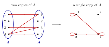
Figure 57: One relation on \(A = {1,2,3,4}\), \(\rho = {(1,1),(3,3),(4,1),(4,3),(4,4)}\), in its two drawings. Left: two copies of \(A\) with arrows from the left copy to the right, as for a function. Right: a single copy of \(A\), the directed graph. Each arrow keeps its start and end, and an arrow from an element to itself becomes a loop. The single-copy drawing is the one to use for a relation on one set, because the three properties below are all about loops, return arrows and short cuts, and those only show up when each element is drawn once.
Reflexivity, symmetry and transitivity
A relation \(\rho\) on a set \(A\) is
(1) reflexive if and only if \(\forall x \in A,\ x \mathrel{\rho} x\).
(2) symmetric if and only if \(\forall x, y \in A,\ x \mathrel{\rho} y \to y \mathrel{\rho} x\).
(3) transitive if and only if \(\forall x, y, z \in A,\ (x \mathrel{\rho} y \text{ and } y \mathrel{\rho} z) \to x \mathrel{\rho} z\).
Each definition has a picture:
| Picture | In symbols | |
|---|---|---|
| reflexive | a loop at \(a\) | \(\forall a \in A,\ a \mathrel{\rho} a\) |
| symmetric | \(a \to b\) above, \(b \to a\) below | \(\forall a, b \in A,\ a \mathrel{\rho} b \to b \mathrel{\rho} a\) |
| transitive | \(a \to b \to c\) along the top, and \(a \to c\) underneath | \(\forall a, b, c \in A,\ a \mathrel{\rho} b \text{ and } b \mathrel{\rho} c \to a \mathrel{\rho} c\) |
Three points about the transitive definition:
- Could have \(x = z\). \(x, y, z\) are any elements of \(A\), not three different ones, so the transitive condition applies with \(z = x\).
- That gives if \(x \mathrel{\rho} y\) and \(y \mathrel{\rho} x\) then \(x \mathrel{\rho} x\), with the weight on the if. Transitivity applied to \(x \to y \to x\) demands the short cut from \(x\) to \(x\), a loop.
- In a transitive relation a two-way pair \(x \rightleftarrows y\) forces loops at both ends (\(y \to x \to y\) gives \(y \mathrel{\rho} y\) as well). So \(x \rightleftarrows y\) with no loops is, on its own, not transitive.
This observation is behind the transitivity counterexamples for disjoint sets (the first one), Diagram 1 and the relation mod 7, and behind the extra hypothesis in the last worked question. It is drawn as Figure 61.
Worked: proper subset on a power set
Questions 1, 2 and 3 from video 30.
Let \(S = \{1,2,3\}\) and consider the relation \(\rho\) defined on the power set of \(S\), \(\mathcal{P}(S)\), by \(X \mathrel{\rho} Y\) if and only if \(X \subset Y\), for all \(X, Y \in \mathcal{P}(S)\).
Q1. True or False: the relation \(\rho\) is reflexive. — False Q2. True or False: the relation \(\rho\) is symmetric. — False Q3. True or False: the relation \(\rho\) is transitive. — True
The reasons for Q2 and Q3: \(X \subset Y \nRightarrow Y \subset X\), and \(X \subset Y\) and \(Y \subset Z \to X \subset Z\) ✓. The power set is \(\mathcal{P}(S) = \{\emptyset, \{1\}, \{2\}, \{3\}, \{1,2\}, \{1,3\}, \{2,3\}, \{1,2,3\}\}\), eight sets. The arrow diagram has a dot for each, with arrows from \(\emptyset\) to all seven other sets, then \(\{1\} \to \{1,2\}\), \(\{1\} \to \{1,2,3\}\) and \(\{1,2\} \to \{1,2,3\}\), and so on: 19 arrows in total.
\(\subset\) is proper subset in this course (sets-and-set-notation), and that is what makes Q1 false. \(X \subset X\) is never true, so there is not a single loop. With \(\subseteq\) instead, Q1 would be true and there would be 27 arrows, the 19 plus a loop at each of the 8 sets. Q2 is false with one witness, \(\emptyset \subset \{1\}\) but \(\{1\} \not\subset \emptyset\).
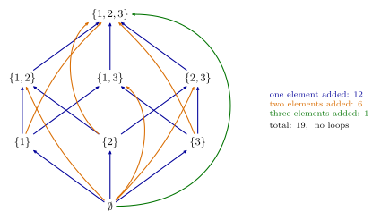
Figure 58: The relation \(X \subset Y\) on \(\mathcal{P}({1,2,3})\) in full, with the sets in layers by size. Blue arrows add one element (12 of them), orange arrows add two (6), and the green arrow adds all three (1): 19 in total. There are no loops, since no set is a proper subset of itself, so the relation is not reflexive. Every arrow points upward and none comes back, so it is not symmetric. Every two-step path has its one-step short cut — the orange and green arrows are exactly those short cuts — so it is transitive.
Worked: disjoint sets
Let \(\rho\) be the relation on \(\mathcal{P}(\mathbb{Z}^{+})\) defined by \(X \mathrel{\rho} Y \leftrightarrow X \cap Y = \emptyset\).
Is \(\rho\) reflexive? \(X \cap X = X\). E.g. \(\{1,2\} \cap \{1,2\} = \{1,2\} \neq \emptyset\), so \(X \mathrel{\not\rho} X\). \(\rho\) is NOT reflexive.
Is \(\rho\) symmetric? Yes. \(X \cap Y = Y \cap X\), so \(\forall X, Y \in \mathcal{P}(\mathbb{Z}^{+})\), if \(X \mathrel{\rho} Y\) then \(Y \mathrel{\rho} X\).
Is \(\rho\) transitive? \(X = \{1\}\), \(Y = \{2\}\), \(Z = \{1\}\): here \(X \mathrel{\rho} Y\) and \(Y \mathrel{\rho} Z\) but \(X \mathrel{\not\rho} Z\). Not transitive. \(X = \{1,2\}\), \(Y = \{3,4\}\), \(Z = \{1,5\}\) also shows not transitive.
The reflexive definition starts \(\forall a \in A\). That quantifier is why one example settles the question. Reflexive is a “for all”, so it fails as soon as one element lacks its loop, even though some elements have one: \(\emptyset \cap \emptyset = \emptyset\), so \(\emptyset \mathrel{\rho} \emptyset\). The first transitivity counterexample uses \(Z = X\), the could have \(x = z\) case: \(\{1\}\) and \(\{2\}\) are related both ways, so transitivity would force \(\{1\} \mathrel{\rho} \{1\}\), which is false. The second shows the same failure with three different sets.
Worked: reading the properties off Diagram 1
Let \(\rho\) be the relation defined by the arrow diagram in Diagram 1.
Diagram 1 has four points \(a, b, c, d\). The arrows are a loop at \(a\), both \(a \to b\) and \(b \to a\), then \(a \to c\), \(a \to d\), \(b \to c\), \(b \to d\), \(c \to d\), and a loop at \(d\). As a set, \[\rho = \{(a,a), (a,b), (b,a), (a,c), (a,d), (b,c), (b,d), (c,d), (d,d)\}.\]
Is \(\rho\) reflexive? No. E.g. \(b \mathrel{\not\rho} b\), or \((b,b) \notin \rho\). Either notation is fine.
Is \(\rho\) symmetric? No. We have \(b \mathrel{\rho} c\) but \(c \mathrel{\not\rho} b\).
Is \(\rho\) transitive? No. We have \(b \mathrel{\rho} a\) and \(a \mathrel{\rho} b\) but \(b \mathrel{\not\rho} b\).
What is missing for each property:
- To make \(\rho\) reflexive: add \((b,b)\) and \((c,c)\).
- To make \(\rho\) symmetric: add \((c,a)\), \((d,a)\), \((c,b)\), \((d,c)\), \((d,b)\).
- To make \(\rho\) transitive: add \((b,b)\).
The three definitions each start with a quantifier, \(\forall a\), \(\forall a, b\) and \(\forall a, b, c\). Each “no” needs only the specific elements that break it.
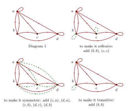
Figure 59: Diagram 1 and what each property would need added, dashed in green. Reflexive: the two missing loops, at \(b\) and \(c\). Symmetric: a return arrow for each of the five one-way arrows. Transitive: only the loop at \(b\), forced by the round trip \(b \to a \to b\) — every other two-step path, such as \(a \to c \to d\) or \(b \to a \to d\), already has its short cut. The transitivity check is the slow one: it means looking at every two-step path, not just at pairs of points.
Worked: an arrow diagram mod 7
Draw an arrow diagram for the relation \(\rho\) on \(\{0,1,2,3,4,5,6\}\) defined by \(x \mathrel{\rho} y\) if and only if \(xy \equiv 1 \pmod 7\).
Working: numbers \(\equiv 1 \pmod 7\) are \(1, 8, 15, 22, 29, 36, \dots\). \(0 \cdot y \not\equiv 1 \pmod 7\), so 0 is related to nothing. \(1 \cdot y \equiv 1 \pmod 7\) (so 1 is related only to 1). The diagram has 0 on its own, loops at 1 and 6, arrows both ways between 2 and 4, and both ways between 3 and 5.
Is \(\rho\) reflexive? No, e.g. \(5 \mathrel{\not\rho} 5\).
Is \(\rho\) symmetric? Yes.
Is \(\rho\) transitive? No. For example \(2 \mathrel{\rho} 4\) and \(4 \mathrel{\rho} 2\) but \(2 \mathrel{\not\rho} 2\).
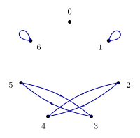
Figure 60: The relation \(xy \equiv 1 \pmod 7\) on \({0, 1, \dots, 6}\). The products that leave remainder 1 are \(1 \cdot 1 = 1\), \(2 \cdot 4 = 8\), \(3 \cdot 5 = 15\) and \(6 \cdot 6 = 36\). Each non-zero number is related to exactly one partner, the number it multiplies with to give 1, and 0 to nothing. Symmetric, because \(xy = yx\). Not reflexive: only 1 and 6 have loops. Not transitive: \(2 \to 4 \to 2\) would need a loop at 2.
Worked: symmetric and transitive, but not reflexive
Prove or disprove the following statement. If a relation \(\rho\) on a set \(A\) is both symmetric and transitive, then \(\rho\) is reflexive.
The statement is false. E.g. \(A = \{1,2\}\), \(\rho = \{(1,1)\}\). The diagram is a loop at 1, and 2 on its own.
\(\rho\) is symmetric and transitive but NOT reflexive (since \(2 \mathrel{\not\rho} 2\)).
- symmetric: \(\forall a, b \in A\) if \(a \mathrel{\rho} b\) then \(b \mathrel{\rho} a\) ✓
- transitive: \(\forall a, b, c \in A\) if \(a \mathrel{\rho} b\) and \(b \mathrel{\rho} c\) then \(a \mathrel{\rho} c\) ✓
The if is the point of the counterexample. Symmetry and transitivity are conditional. They say what must happen if some arrows are present, and they are satisfied without argument wherever those arrows are absent. The only arrow in \(\rho\) is the loop \((1,1)\). Its “return arrow” and its “short cut” are the same loop, so both conditions hold. Element 2 has no arrows at all, so neither condition ever mentions it, and nothing forces a loop there.
One more hypothesis repairs it:
If we also knew that for each \(x \in A\), \(x \mathrel{\rho} y\) for some \(y \in A\), then the statement becomes true.
With that extra hypothesis, take any \(x\). It has an arrow to some \(y\). Symmetry gives the arrow back, and transitivity on \(x \to y \to x\) gives the loop at \(x\). The picture is \(x \rightleftarrows y\) with a loop at each end. This is the if \(x \mathrel{\rho} y\) and \(y \mathrel{\rho} x\) then \(x \mathrel{\rho} x\) observation from the definitions above, and it is the proof that people write without the extra hypothesis. The step “take a \(y\) with \(x \mathrel{\rho} y\)” is exactly where it breaks, because such a \(y\) need not exist.
Figure 61: Why symmetric and transitive do not make a relation reflexive, and what would. Left: \(\rho = {(1,1)}\) on \({1, 2}\) is symmetric and transitive but not reflexive; 2 has no arrows, so neither condition ever says anything about it. Right: once \(x\) has an arrow to some \(y\), symmetry supplies \(y \to x\), and transitivity along \(x \to y \to x\) forces the loop at \(x\) (and along \(y \to x \to y\), the loop at \(y\)). The forced arrows are dashed. The loop depends on \(x\) being related to something.
See also
- relations-on-sets — relations as sets of pairs, the notation \(x \mathrel{\rho} y\), and the two ways to draw one
- reflexive-symmetric-and-transitive-relations — the three properties, their pictures, and how to prove and disprove each
- functions-on-general-sets — functions as the special relations with one arrow out of each element
- 2026-09-15-countable-and-uncountable-sets — Lecture 22 · 2026-09-21-equivalence-relations — Lecture 24
- practice-problems — §29 · practice-problems — §30, with full worked solutions
Week 9
Lecture 24 — Equivalence Relations
Equivalence relations, their classes, and why the classes cut the set into a partition. Pre-work: Video 031 (Equivalence Relations). The definition and how to prove or disprove it are collected in equivalence-relations, and classes, partitions and the two-way link between them in equivalence-classes-and-partitions. The three properties come from reflexive-symmetric-and-transitive-relations.
Goals
- Know how to prove or disprove that a relation is an equivalence relation.
- Understand equivalence classes.
- Understand the connection between equivalence relations and partitions.
All three in one sentence:
If \(R\) is an equivalence relation on a set \(A\), then the equivalence classes of \(R\) partition \(A\).
Figure 62: A set \(A\) cut into the equivalence classes of a relation on it. Every element of \(A\) lies in exactly one region. Each region is named after one of the elements in it, written in square brackets: \([a]\) is the region that \(a\) is in. The regions cover \(A\) and no two overlap, and that is what a partition is.
Three questions to start with
Are there any equivalence relations apart from congruence mod \(n\) and equality? Yes. Fractions are one. Take pairs of positive integers and relate
\[(a,b) \sim (c,d) \quad\text{if and only if}\quad ad = bc,\]
which is the condition \(\dfrac{a}{b} = \dfrac{c}{d}\) written without division. Then \(\frac12 = \frac24 = \frac36 = \cdots\) says that \((1,2)\), \((2,4)\) and \((3,6)\) are all related: three pairs in one class. A positive rational number is a whole class of pairs. The relation is worked through in equivalence-relations.
What exactly is the equivalence class \([a]\)? The set of everything related to \(a\). See Equivalence classes.
Why does the set of equivalence classes form a partition, and given a partition, how do we get an equivalence relation? The first is Two classes are equal or disjoint, and the second is From a partition to an equivalence relation.
The definition
For a relation \(\rho\) on a set \(A\) (reflexive-symmetric-and-transitive-relations):
| Property | Condition |
|---|---|
| reflexive | \(\forall x \in A,\ x \mathrel{\rho} x\) |
| symmetric | \(\forall x, y \in A,\ x \mathrel{\rho} y \to y \mathrel{\rho} x\) |
| transitive | \(\forall x, y, z \in A,\ (x \mathrel{\rho} y \text{ and } y \mathrel{\rho} z) \to x \mathrel{\rho} z\) |
A relation is an equivalence relation if and only if it is reflexive, symmetric and transitive.
Worked: the sum is rational
Let \(\rho\) be the relation on \(\mathbb{R}\) defined by: for all \(x, y \in \mathbb{R}\), \(x \mathrel{\rho} y\) if and only if \(x + y \in \mathbb{Q}\). Is \(\rho\) an equivalence relation?
No. \(\rho\) is not reflexive.
Take \(x = \sqrt2 \in \mathbb{R}\). Then \(x + x = \sqrt2 + \sqrt2 = 2\sqrt2 \notin \mathbb{Q}\), so \(\sqrt2 \mathrel{\not\rho} \sqrt2\). \(\therefore \rho\) is not an equivalence relation.
Reflexive is a “for all” statement, \(\forall x \in A,\ x \mathrel{\rho} x\), so a single \(x\) that fails disproves it. An equivalence relation needs all three properties, so one failed property, shown by one witness, settles the question. There is no need to look at the other two.
For the record, \(\rho\) is symmetric, because \(x + y = y + x\). It is not transitive: \(\sqrt2 \mathrel{\rho} {-\sqrt2}\) and \(-\sqrt2 \mathrel{\rho} \sqrt2\), since both sums are \(0\), but \(\sqrt2 \mathrel{\not\rho} \sqrt2\). That is the forced loop of reflexive-symmetric-and-transitive-relations again.
Worked: the difference is rational
Let \(\tau\) be the relation on \(\mathbb{R}\) defined by: for all \(x, y \in \mathbb{R}\), \(x \mathrel{\tau} y\) if and only if \(x - y \in \mathbb{Q}\). Is \(\tau\) an equivalence relation?
Yes. The proof has three parts, one for each property.
(1) Reflexive. Let \(x \in \mathbb{R}\). (Think: is \(x \mathrel{\tau} x\)?) \(x - x = 0 \in \mathbb{Q}\), since \(0 = \frac01\). So \(\tau\) is reflexive.
(2) Symmetric. Let \(x, y \in \mathbb{R}\) and suppose \(x \mathrel{\tau} y\). Then \(x - y \in \mathbb{Q}\), so \(x - y = \dfrac{a}{b}\) for some \(a, b \in \mathbb{Z}\), \(b \neq 0\). \[y - x = -(x - y) = -\left(\frac{a}{b}\right) = \frac{-a}{b}.\] Since \(-a \in \mathbb{Z}\) we have \(y - x \in \mathbb{Q}\), so \(y \mathrel{\tau} x\). \(\therefore \tau\) is symmetric.
(3) Transitive. Let \(x, y, z \in \mathbb{R}\) and suppose \(x \mathrel{\tau} y\) and \(y \mathrel{\tau} z\). Thus \(x - y = \dfrac{a}{b}\) and \(y - z = \dfrac{c}{d}\) for some \(a, b, c, d \in \mathbb{Z}\), \(b \neq 0\), \(d \neq 0\). \[\text{Now } x - z = (x - y) + (y - z) = \frac{a}{b} + \frac{c}{d} = \frac{ad + bc}{bd}.\] Since \(a, b, c, d \in \mathbb{Z}\), \(ad + bc,\ bd \in \mathbb{Z}\). Also \(bd \neq 0\). \(\therefore x - z \in \mathbb{Q}\), so \(x \mathrel{\tau} z\). \(\therefore \tau\) is transitive.
Three things to copy from this proof:
- Start each part by asking what the property says for this relation. For reflexive that is “is \(x \mathrel{\tau} x\)?”, which is “is \(x - x \in \mathbb{Q}\)?”.
- Each part unfolds the definition. “\(x - y \in \mathbb{Q}\)” is turned into \(x - y = \frac{a}{b}\) with \(a, b \in \mathbb{Z}\), \(b \neq 0\) (rational-and-irrational-numbers), worked on, and folded back up into “\(\in \mathbb{Q}\)”.
- New letters for the second fraction. Part (3) uses \(\frac{c}{d}\) for \(y - z\). Writing \(\frac{a}{b}\) again would claim the two differences are equal.
The step that makes part (3) work is \(x - z = (x - y) + (y - z)\): the middle term cancels. For sums there is no such identity, which is where \(\rho\) goes wrong.
Figure 63: The same five real numbers under the two relations. Left, \(x \mathrel{\rho} y \leftrightarrow x + y \in \mathbb{Q}\). Only 0 and 1 have loops. There is none at \(\sqrt2\) because \(\sqrt2 + \sqrt2\) is irrational, so \(\rho\) is not reflexive, and the three missing loops are dashed. Right, \(x \mathrel{\tau} y \leftrightarrow x - y \in \mathbb{Q}\). Every number has a loop because \(x - x = 0\), and the numbers fall into three separate clusters with every arrow present inside a cluster and none between clusters. That clustered shape is what an equivalence relation looks like.
Partitions
Two sets \(X\) and \(Y\) are disjoint if and only if \(X \cap Y = \emptyset\).
A collection of sets is mutually disjoint if each pair of distinct sets in the collection is disjoint.A partition of a set \(S\) is a collection of non-empty and mutually disjoint subsets of \(S\) whose union is \(S\).
The subsets in a partition are sometimes called parts.
This is the definition from sets-and-set-notation with two new words, mutually disjoint and parts. Three conditions: the pieces are non-empty, no two overlap, and together they cover \(S\).
The positive integers by remainder. \[\big\{\{1,4,7,\dots\},\ \{2,5,8,\dots\},\ \{3,6,9,\dots\}\big\} \text{ is a partition of } \mathbb{Z}^{+}.\] The three parts are the positive integers sorted by remainder on division by 3. A partition is always a partition of some set, here \(\mathbb{Z}^{+}\), and naming that set is part of the statement.
One set, two partitions. Let \(S = \{x_1, x_2, x_3, x_4, x_5, x_6, x_7, x_8, x_9\}\).
- \(\big\{\{x_1, x_2, x_3\},\ \{x_4, x_5\},\ \{x_6, x_7, x_8, x_9\}\big\}\) is a partition of \(S\) with 3 parts.
- \(\big\{\{x_1, x_2\},\ \{x_3, x_4\},\ \{x_5, x_8, x_9\},\ \{x_6, x_7\}\big\}\) is another partition of \(S\), with 4 parts.
One set has many partitions. The parts need not be the same size, and their elements need not be next to each other in any listing: \(\{x_5, x_8, x_9\}\) is a part.
Mutually disjoint, and not. Let \(W = \{1,2,3\}\), \(X = \{4,5,6\}\), \(Y = \{6,7,8\}\), \(Z = \{7,8,9,10\}\).
- \(W\), \(X\) and \(Z\) are mutually disjoint.
- \(W\), \(X\) and \(Y\) are not mutually disjoint, because \(X \cap Y = \{6\}\). One overlapping pair is enough, even though \(W\) is disjoint from both of the others.
- \(\{W, X, Z\}\) is a partition of \(\{1,2,3,4,5,6,7,8,9,10\}\) with 3 parts.
Figure 64: The four sets \(W\), \(X\), \(Y\) and \(Z\) on the numbers 1 to 10. \(W\), \(X\) and \(Z\) sit side by side and share no number, so they are mutually disjoint, and between them they use every number from 1 to 10, so \({W, X, Z}\) is a partition with three parts. \(Y\) shares 6 with \(X\) and shares 7 and 8 with \(Z\). A collection that contains \(Y\) together with \(X\) or \(Z\) is not mutually disjoint, however many of its other pairs are disjoint. The shared numbers are shaded, 6 in green and 7 and 8 in purple.
Equivalence classes
Let \(\rho\) be an equivalence relation on a set \(S\). For each \(a \in S\), the equivalence class of \(a\) is \[[a] = \{x \in S : x \mathrel{\rho} a\},\] the set of elements related to \(a\).
The equivalence classes of an equivalence relation on a set \(S\) form a partition of \(S\).
Congruence mod 3. For \(m \mathrel{T} n \leftrightarrow m \equiv n \pmod 3\) on \(\mathbb{Z}\) there are three classes:
\[[0] = \{\dots, -6, -3, 0, 3, 6, \dots\}, \qquad [1] = \{\dots, -5, -2, 1, 4, 7, \dots\}, \qquad [2] = \{\dots, -4, -1, 2, 5, 8, \dots\}.\]
Also \([0] = [3] = [-6]\). A class is a set, and the bracket only says which element was used to name it. Every element of a class names that same class, so a class with infinitely many elements has infinitely many names.
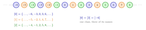
Figure 65: The integers from \(-6\) to 8, coloured by remainder on division by 3. Each colour is one equivalence class of \(m \equiv n \pmod 3\). The classes are spread along the number line, every third integer, and each integer has exactly one colour, so the three classes partition \(\mathbb{Z}\). The line at the right gives one class three of its names: \([0]\), \([3]\) and \([-6]\) are the same set, named after three different elements of it.
Same parity. The relation \(\rho\) on \(\mathbb{Z}\) defined by “\(m \mathrel{\rho} n\) if and only if \(m\) and \(n\) have the same parity” is an equivalence relation. Its equivalence classes are
\[\mathbb{Z}^{even} = \{\dots, -4, -2, 0, 2, 4, \dots\} \qquad\text{and}\qquad \mathbb{Z}^{odd} = \{\dots, -3, -1, 1, 3, 5, \dots\},\]
and these two classes partition \(\mathbb{Z}\).
As an arrow diagram, the inside of a class has a loop at every element and arrows both ways between every pair. All of its elements are related to each other and to themselves, and none is related to anything outside.
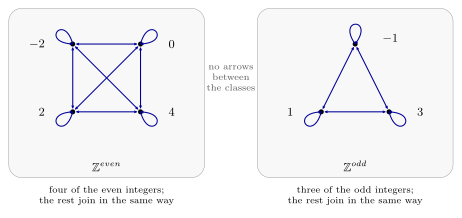
Figure 66: Inside one equivalence class every element is related to every other, in both directions, and to itself. Between two different classes there are no arrows at all. Shown for the relation same parity on \(\mathbb{Z}\), with four of the even integers and three of the odd ones. Each double-headed line stands for one arrow each way.
Worked: the classes of \(\tau\)
\(\tau\) is the equivalence relation from before: for all \(x, y \in \mathbb{R}\), \(x \mathrel{\tau} y\) if and only if \(x - y \in \mathbb{Q}\).
(a) Describe the equivalence class \([1]\).
\[1 \mathrel{\tau} y \ \leftrightarrow\ 1 - y \in \mathbb{Q} \ \leftrightarrow\ y \in \mathbb{Q}, \qquad\text{so}\qquad [1] = \mathbb{Q}.\]
The method is to ask which \(y\) are related to 1 and unfold the definition until it is a plain condition on \(y\). The class is defined as the \(x\) with \(x \mathrel{\tau} 1\), and this works with \(1 \mathrel{\tau} y\) instead. For an equivalence relation the order makes no difference, because it is symmetric.
(b) State three elements that are in the equivalence class \([\sqrt2]\).
- \(\sqrt2 \in [\sqrt2]\), because \(\sqrt2 - \sqrt2 = 0 \in \mathbb{Q}\), so \(\sqrt2 \mathrel{\tau} \sqrt2\).
- \(1 + \sqrt2 \in [\sqrt2]\), because \(\sqrt2 - (1 + \sqrt2) = -1 \in \mathbb{Q}\).
- \(-3 + \sqrt2 \in [\sqrt2]\), because \(\sqrt2 - (-3 + \sqrt2) = 3 \in \mathbb{Q}\).
The whole class is
\[[\sqrt2] = \{y + \sqrt2 : y \in \mathbb{Q}\}.\]
The first element is the standard one. \(a\) is always in \([a]\), because the relation is reflexive.
(c) Is \([\sqrt2] = [-\sqrt2]\)?
\(\sqrt2 - (-\sqrt2) = 2\sqrt2 \notin \mathbb{Q}\), so \(\sqrt2 \mathrel{\not\tau} {-\sqrt2}\). Therefore \([\sqrt2] \neq [-\sqrt2]\).
To compare two classes, test their two names against each other. Related names give the same class, and unrelated names give different classes. Why that is enough is the next section.
So \(\mathbb{R}\) is cut into classes, of which \([1] = \mathbb{Q}\), \([\sqrt2]\) and \([-\sqrt2]\) are three.
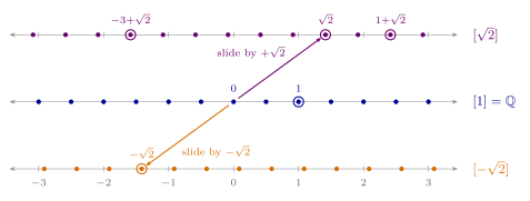
Figure 67: Three of the equivalence classes of \(\tau\), each on its own copy of the real line. A class cannot be drawn in full, so only the numbers a multiple of \(\tfrac12\) away from the class’s name are shown. \([1]\) is \(\mathbb{Q}\). \([\sqrt2] = {y + \sqrt2 : y \in \mathbb{Q}}\) is \(\mathbb{Q}\) slid \(\sqrt2\) to the right, and \([-\sqrt2]\) is \(\mathbb{Q}\) slid \(\sqrt2\) to the left. The ringed points are 1, the three elements found for \([\sqrt2]\), and \(-\sqrt2\). No point of one line is directly above a point of another, since a real number is in only one class.
Each class of \(\tau\) is a copy of \(\mathbb{Q}\), so it is countable, and \(\mathbb{R}\) is not (countable-and-uncountable-sets). So there are infinitely many classes besides these three.
Two classes are equal or disjoint
True or false: if the equivalence class \([a]\) is equal to the equivalence class \([b]\), then \(b \in [a]\).
True. \(b \in [b]\) because the relation is reflexive. So if \([a] = [b]\) then
\[b \in [b] = [a].\]
The result behind it:
Important result. If \(\rho\) is an equivalence relation on a set \(S\), and \(a, b \in S\), then either \[[a] = [b] \qquad \text{or} \qquad [a] \cap [b] = \emptyset.\] If \(a \mathrel{\rho} b\) the classes are equal, and if \(a \mathrel{\not\rho} b\) they are disjoint.
Two classes are either the same set or have nothing in common. They never partly overlap.
This is why the equivalence classes form a partition:
- the classes are non-empty, since \(a \in [a]\);
- every element is in a class, its own, so their union is \(S\);
- two different classes are disjoint, by the result.
The proof of the result, with a picture, is in equivalence-classes-and-partitions.
Worked: a relation defined with “or”
The relation \(\sigma\) on \(\mathbb{Z}\) is defined by \(m \mathrel{\sigma} n \leftrightarrow (8 \text{ divides } m - n) \text{ or } (8 \text{ divides } m + n)\). It is an equivalence relation. Describe its equivalence classes.
The proof that it is an equivalence relation is below. The classes are worked out in 2026-09-22-partial-order-relations: there are five of them.
From a partition to an equivalence relation
The link also runs the other way.
Given any partition of a set \(S\), we can define an equivalence relation on \(S\) by taking two elements to be related if and only if they are in the same part of the partition. The parts of the partition are then the equivalence classes of that relation.
Any partition defines an equivalence relation, and any equivalence relation defines a partition.
Example. Let \(S = \{1,2,3,4,5,6\}\) with the partition \(\big\{\{1,2,3\}, \{4,5\}, \{6\}\big\}\). The equivalence relation \(R\) on \(S\) built from this partition is
\[R = \{(1,1), (1,2), (1,3), (2,1), (2,2), (2,3), (3,1), (3,2), (3,3), (4,4), (4,5), (5,5), (5,4), (6,6)\}.\]
\(R\) has three equivalence classes:
\[[1] = \{1,2,3\} = [2] = [3], \qquad [4] = \{4,5\} = [5], \qquad [6] = \{6\}.\]
A part with \(k\) elements contributes all \(k \times k\) pairs of its elements, loops included, so \(R\) has \(3^2 + 2^2 + 1^2 = 14\) pairs. Reading the classes back off \(R\) returns the partition it was built from.
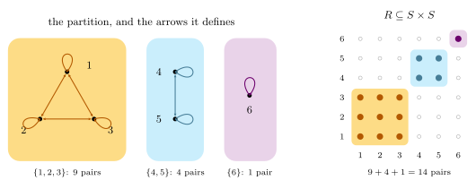
Figure 68: From a partition to the relation it defines. Left: the three parts of \(S = {1, \dots, 6}\), and inside each part every arrow, since two elements are related exactly when they are in the same part. Right: the same relation as a set of points in the grid \(S \times S\), the first coordinate across and the second up. Each part gives a solid square block on the diagonal, \(3 \times 3\), \(2 \times 2\) and \(1 \times 1\), so \(R\) has \(9 + 4 + 1 = 14\) pairs. Yellow marks \({1,2,3}\) and its nine pairs, cyan \({4,5}\) and its four, purple \({6}\) and \((6,6)\).
Question. Consider the partition of the integers given by \(\{\mathbb{Z}^{-}, \{0\}, \mathbb{Z}^{+}\}\). Describe an equivalence relation that corresponds to this partition.
Answered in 2026-09-22-partial-order-relations.
See also
- equivalence-relations — the definition, the proof template, and these relations side by side
- equivalence-classes-and-partitions — classes, why two classes are equal or disjoint, and partitions to relations and back
- reflexive-symmetric-and-transitive-relations — the three properties an equivalence relation needs
- sets-and-set-notation — partitions as first defined
- modular-arithmetic — congruence, the standard source of equivalence relations
- 2026-09-17-relations-reflexivity-symmetry-transitivity — Lecture 23 · 2026-09-22-partial-order-relations — Lecture 25
- practice-problems — §31, with full worked solutions
Lecture 25 — Partial Order Relations
Antisymmetry, comparable elements, partial and total orders, and Hasse diagrams. Pre-work: Video 032 (Partial Order Relations). The new property is collected in antisymmetric-relations, comparable elements and the two kinds of order in partial-order-relations, and the simplified drawing in hasse-diagrams. The note starts with two questions left over from 2026-09-21-equivalence-relations.
Goals
- Understand antisymmetry, comparable, partial order, total order in the context of relations.
- Learn how to prove a relation is antisymmetric.
- Learn how to prove a relation is a partial/total order.
- Learn how to draw a Hasse diagram.
Two things to have straight before starting:
- Antisymmetric does not mean “not symmetric”. A relation can be both, either one, or neither. Symmetric against antisymmetric has one of each.
- \(2 \mid 6\) is a statement. “2 divides 6” is true or false. It is not a number, and in particular it is not the fraction \(\frac26\) (divisibility-and-factorisation). The relation “divides” is the subject of a worked proof below.
Two questions carried over from Lecture 24
The classes of \(\sigma\)
The relation \(\sigma\) on \(\mathbb{Z}\) defined by \(m \mathrel{\sigma} n \leftrightarrow (8 \text{ divides } m - n) \text{ or } (8 \text{ divides } m + n)\) is an equivalence relation. Describe the equivalence classes of \(\sigma\).
Work out one class at a time, starting from the definition of a class:
\[\begin{aligned} [1] &= \{n \in \mathbb{Z} : 8 \mid (1 - n) \text{ or } 8 \mid (1 + n)\} \\ &= \{n \in \mathbb{Z} : n \equiv 1 \text{ or } 7 \pmod 8\} && = [7] \\[4pt] [2] &= \{n \in \mathbb{Z} : 8 \mid (2 - n) \text{ or } 8 \mid (2 + n)\} \\ &= \{n \in \mathbb{Z} : n \equiv 2 \text{ or } 6 \pmod 8\} && = [6] \\[4pt] [3] &= \{n \in \mathbb{Z} : n \equiv 3 \text{ or } 5 \pmod 8\} && = [5] \\[4pt] [4] &= \{n \in \mathbb{Z} : 8 \mid (4 - n) \text{ or } 8 \mid (4 + n)\} \\ &= \{n \in \mathbb{Z} : n \equiv 4 \pmod 8\} \\[4pt] [0] &= \{n \in \mathbb{Z} : n \equiv 0 \pmod 8\} \end{aligned}\]
For example 1, 9, 7 and 17 are four elements of \([1]\).
So \(\sigma\) has five classes. The reason:
- \(8 \mid (a - n)\) says \(n \equiv a \pmod 8\), and \(8 \mid (a + n)\) says \(n \equiv -a \pmod 8\). So \([a]\) collects the integers congruent to \(a\) together with the integers congruent to \(-a\).
- Mod 8, \(-1 \equiv 7\), \(-2 \equiv 6\) and \(-3 \equiv 5\), which joins the remainders in pairs.
- But \(-4 \equiv 4\) and \(-0 \equiv 0\), so \([4]\) and \([0]\) get nothing extra.
Every integer has exactly one remainder from 0 to 7, so every integer is in exactly one of the five classes, as it must be.
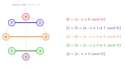
Figure 69: The eight remainders mod 8 on a clock face. Congruence mod 8 on its own has eight classes, one for each remainder. The relation \(\sigma\) also relates \(n\) to everything congruent to \(-n\), and replacing a remainder by its negative is the left-to-right flip of the clock. So each remainder is joined to its mirror image: 1 with 7, 2 with 6, 3 with 5. The remainders 0 and 4 lie on the mirror line and are their own images. That leaves five classes.
The proof that \(\sigma\) is an equivalence relation is in 2026-09-21-equivalence-relations.
A relation for the partition by sign
Any partition defines an equivalence relation: two elements are related if and only if they are in the same part (2026-09-21-equivalence-relations).
Consider the partition of the integers given by \(\{\mathbb{Z}^{-}, \{0\}, \mathbb{Z}^{+}\}\). Describe an equivalence relation that corresponds to this partition.
Define \(\tau\) by: for all \(a, b \in \mathbb{Z}\),
\[a \mathrel{\tau} b \ \longleftrightarrow\ a, b \text{ both positive} \quad\text{or}\quad a = b = 0 \quad\text{or}\quad a, b \text{ both negative}.\]
The condition has one alternative for each part. The middle part has one element, so “both in \(\{0\}\)” becomes \(a = b = 0\).
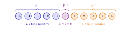
Figure 70: The partition \({\mathbb{Z}^{-}, {0}, \mathbb{Z}^{+}}\) of the integers, shown from \(-5\) to 5, and the relation it defines. Two integers are related exactly when they have the same colour. So \(-4 \mathrel{\tau} -1\) and \(2 \mathrel{\tau} 5\), the only thing related to 0 is 0, and no negative integer is related to a positive one.
Antisymmetry
Definition. A relation \(R\) on a set \(S\) is antisymmetric if and only if \[\forall a, b \in S,\ (a \mathrel{R} b \text{ and } b \mathrel{R} a) \to (a = b).\]
There are two equivalent ways to write it:
\[\forall a, b \in S,\ (a \neq b) \to {\sim}(a \mathrel{R} b \text{ and } b \mathrel{R} a)\]
\[\forall a, b \in S,\ (a \mathrel{R} b \text{ and } a \neq b) \to {\sim}(b \mathrel{R} a)\]
The first form is the easiest for proving a relation antisymmetric. The third is the most intuitive.
All three say the same thing about the arrow diagram: there is no pair of different elements with arrows both ways.
- The first reads it as “if you do find arrows both ways, the two ends were the same element all along”, so the pair of arrows is really one loop.
- The third reads it as “an arrow from \(a\) to a different element \(b\) has no return”.
- Loops are not restricted at all.
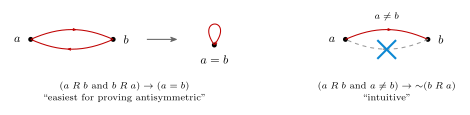
Figure 71: Antisymmetry in two pictures. Left, the first definition: arrows both ways between \(a\) and \(b\) are only possible if \(a\) and \(b\) are the same element, in which case the picture is a single dot with a loop. This is the form to use in a proof. Right, the third definition: an arrow from \(a\) to a different element \(b\) rules out the arrow back from \(b\) to \(a\). This is the form to picture.
Examples.
- \(\leq\) on \(\mathbb{R}\) is antisymmetric: for all \(x, y \in \mathbb{R}\), \((x \leq y \text{ and } y \leq x) \to (x = y)\).
- So are \(<\), \(>\) and \(\geq\) on \(\mathbb{R}\).
- “Divides” is antisymmetric on \(\mathbb{Z}^{+}\). It is proved below.
- \(\subseteq\) on any set \(S\) of sets is antisymmetric: for all \(X, Y \in S\), \((X \subseteq Y \text{ and } Y \subseteq X) \to (X = Y)\). This is the double-containment rule for showing two sets are equal (sets-and-set-notation).
Why \(<\) counts, and why “divides” needs \(\mathbb{Z}^{+}\) and not \(\mathbb{Z}\), are in antisymmetric-relations.
Worked: symmetric against antisymmetric
Symmetric says every arrow has a return: \(\forall a, b \in A,\ a \mathrel{\rho} b \to b \mathrel{\rho} a\). Antisymmetric says no arrow between different elements has one: \(\forall a, b \in S,\ (a \mathrel{R} b \text{ and } b \mathrel{R} a) \to (a = b)\).
Match each of the four arrow diagrams with the description of its relation.
A. Both symmetric and antisymmetric
B. Symmetric but not antisymmetric
C. Antisymmetric but not symmetric
D. Neither symmetric nor antisymmetric
Each diagram has three dots.
| The arrows | Answer | Why | |
|---|---|---|---|
| Diagram 1 | both ways between the first and second dots; one arrow from the second to the third; a loop at the third | D | the two-way pair joins different elements, so not antisymmetric; the single arrow has no return, so not symmetric |
| Diagram 2 | a loop at each of two dots; the third dot has no arrows | A | the only arrows are loops, which break neither property |
| Diagram 3 | both ways between the first and second dots, and both ways between the second and third; a loop at the third | B | every arrow has a return, so symmetric; the two-way pairs join different elements, so not antisymmetric |
| Diagram 4 | one arrow from the first dot to the second, and one from the second to the third; a loop at the third | C | neither single arrow has a return, so not symmetric; there is no two-way pair, so antisymmetric |
Diagram 2 is the one that shows antisymmetric is not the opposite of symmetric. Its only arrows are loops. A loop is its own return, so the relation is symmetric. There are no arrows between different elements, so nothing can break antisymmetry.
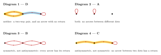
Figure 72: Four relations on three points, with their answers. Between two different dots there are three possibilities: no arrow, one arrow, or arrows both ways. A single arrow breaks symmetry, and arrows both ways break antisymmetry. Diagram 1 has one of each, the single arrow shaded cyan and the two-way pair yellow, so it is neither. Diagram 2 has no arrows between different dots, so it is both. Diagram 3 has only two-way pairs, so it is symmetric and not antisymmetric. Diagram 4 has only single arrows, so it is antisymmetric and not symmetric. The loops play no part in any of the four answers.
Comparable and non-comparable elements
If \(R\) is a relation on a set \(S\), then two elements \(a, b \in S\) are comparable if and only if \(a \mathrel{R} b\) or \(b \mathrel{R} a\).
Comparable means related in some direction.
Example. A relation \(R\) on six points \(a\) to \(f\), with arrows \(a \to c\) and \(c \to a\), \(c \to e\), \(b \to a\), \(b \to e\), \(f \to b\), \(b \to d\), and loops at \(b\) and at \(e\):
| Comparable | Noncomparable |
|---|---|
| \(a\) and \(c\) | \(a\) and \(e\) |
| \(a\) and \(b\) | \(a\) and \(d\) |
| \(c\) and \(e\) | \(a\) and \(f\) |
| \(b\) and \(e\) | \(b\) and \(c\) |
| \(b\) and \(d\) | \(c\) and \(d\) |
| \(b\) and \(f\) | \(c\) and \(f\) |
| \(d\) and \(e\) | |
| \(b\) and \(b\) | \(d\) and \(f\) |
| \(e\) and \(e\) | \(e\) and \(f\) |
What the two columns show:
- Direction does not matter. \(a\) and \(b\) are comparable because of the arrow \(b \to a\). One arrow either way is enough.
- Comparable means one arrow, not a path. \(a\) and \(e\) are noncomparable although \(a \to c \to e\) is a path, because there is no arrow between them. This \(R\) is not transitive.
- An element is comparable with itself only if it has a loop. Only \(b\) and \(e\) are comparable with themselves.
- The 15 pairs of different points split 6 and 9.
This \(R\) is not a partial order: \(a\) and \(c\) are joined both ways, and four points have no loop. The definition of comparable does not need one.
Figure 73: The relation \(R\) on six points, with three pairs highlighted. \(c\) and \(e\), in yellow, are comparable: there is an arrow \(c \to e\). \(b\) is comparable with itself, since it has a loop. \(a\) and \(d\), in cyan, are not comparable: no arrow joins them in either direction. Two points are comparable when at least one arrow joins them, whichever way it points.
Worked: comparable sets
In the partial order relation defined on the power set \(\mathcal{P}(\mathbb{Z})\) of \(\mathbb{Z}\) by \(X \mathrel{\rho} Y\) iff \(X \subseteq Y\), which of the following are comparable elements?
| Answer | Why | ||
|---|---|---|---|
| (a) | 7 and 9 | not elements of \(\mathcal{P}(\mathbb{Z})\) | 7 and 9 are integers, not sets of integers, so the relation is not defined on them |
| (b) | \(\{7\}\) and \(\{9\}\) | non-comparable | neither is a subset of the other |
| (c) | \(\{7\}\) and \(\{7,9\}\) | comparable | \(\{7\} \subseteq \{7,9\}\) |
| (d) | \(\{1,2,3\}\) and \(\{1,2,4\}\) | non-comparable | \(3 \notin \{1,2,4\}\) and \(4 \notin \{1,2,3\}\), so neither contains the other |
So the answer is (c). Two traps:
- In (a), the elements of \(\mathcal{P}(\mathbb{Z})\) are sets of integers. That is the element-versus-subset distinction of sets-and-set-notation.
- In (d), the two sets overlap in \(\{1,2\}\). Overlapping is not being comparable.
Partial and total orders
A relation \(R\) on a set \(S\) is a partial order relation if and only if \(R\) is
- reflexive;
- antisymmetric; and
- transitive.
A relation \(R\) on a set \(S\) is a total order relation if and only if \(R\) is
- reflexive;
- antisymmetric;
- transitive; and
- any two elements of \(S\) are comparable.
A total order is a partial order plus condition 4. So:
- Any total order relation is a partial order relation.
- A partial order relation is a total order relation if and only if every two elements are comparable.
As arrow diagrams, a total order is a single column: a loop at each element and an arrow from each element to every element above it. A partial order that is not total has at least one pair of elements with no arrow between them.
Figure 74: Two orders as arrow diagrams. Left, a total order on five elements: a loop at each, and an arrow from each element to every element above it, ten in all. Every two elements are joined by an arrow, so every two are comparable. Right, a partial order that is not total: the same column and a sixth element off to the side, above the bottom element and below the top one. It is joined to nothing else in the column. The two elements shaded cyan are one of the three pairs that are not comparable.
Worked: “divides” is a partial order
(a) Prove that the relation “divides” on \(\mathbb{Z}^{+}\) is a partial order relation.
(b) Is the relation “divides” on \(\mathbb{Z}^{+}\) a total order relation?
Name the relation and unfold it: for all \(a, b \in \mathbb{Z}^{+}\),
\[a \mathrel{\tau} b \leftrightarrow a \mid b \qquad (\text{that is, } b = ak \text{ for some } k \in \mathbb{Z}).\]
(a)
Reflexive. Let \(a \in \mathbb{Z}^{+}\). Since \(a = a \cdot 1\) we have \(a \mid a\), so \(\tau\) is reflexive.
Antisymmetric. Let \(a, b \in \mathbb{Z}^{+}\) and suppose \(a \mathrel{\tau} b\) and \(b \mathrel{\tau} a\). (Goal: show \(a = b\).) Thus \(b = ak\) for some \(k \in \mathbb{Z}\) and \(a = b\ell\) for some \(\ell \in \mathbb{Z}\). \[\text{Now } b = ak = (b\ell)k = b(\ell k), \qquad\text{so}\qquad 1 = \ell k.\] (The \(b\) can be cancelled because \(b \in \mathbb{Z}^{+}\), so \(b \neq 0\).) Note \(\ell > 0\) and \(k > 0\) since \(a, b > 0\). Thus \(\ell = k = 1\), so \(a = b\). \(\therefore \tau\) is antisymmetric.
Transitive. Let \(a, b, c \in \mathbb{Z}^{+}\) and suppose \(a \mathrel{\tau} b\) and \(b \mathrel{\tau} c\). Thus \(b = ak\) and \(c = b\ell\) for some \(k, \ell \in \mathbb{Z}\). Hence \(c = (ak)\ell = a(k\ell)\). Since \(k\ell \in \mathbb{Z}\) we have \(a \mid c\), that is, \(a \mathrel{\tau} c\). So \(\tau\) is transitive.
\(\therefore \tau\) is a partial order.
(b) Not a total order, since \(2 \mathrel{\not\tau} 3\) and \(3 \mathrel{\not\tau} 2\).
Points to notice:
- State the goal. The antisymmetric part begins by writing down where the first form of the definition is heading: show \(a = b\).
- Where \(\mathbb{Z}^{+}\) is needed. The step from \(\ell k = 1\) to \(\ell = k = 1\) uses that both are positive. On all of \(\mathbb{Z}\), \(\ell = k = -1\) is also possible, and the proof fails (antisymmetric-relations).
- One pair is enough for (b). \(2 \nmid 3\) and \(3 \nmid 2\), so 2 and 3 are not comparable. “Any two elements are comparable” is a “for all”, and one pair that fails disproves it.
- The set matters. On \(\{1, 2, 4, 8, 16\}\) each number divides the next, every two are comparable, and “divides” is a total order there.
Hasse diagrams
A Hasse diagram for a partial order relation is obtained from its arrow diagram by:
- placing the elements so that all the arrows point upwards;
- deleting the loops (the arrows from elements to themselves);
- deleting the arrows which are implied by the transitive property;
- deleting the direction indicators on the arrows.
A Hasse diagram is sufficient to define a partial order relation.
Example. The six-element partial order of Figure 74, with the column named \(a\), \(b\), \(c\), \(d\), \(e\) from the bottom and \(f\) at the side. The arrow \(a \to c\) is implied by \(a \to b\) and \(b \to c\), so it is one that step 3 deletes. What is left at the end is \(a\), \(b\), \(c\), \(d\), \(e\) in a vertical line joined by four segments, and \(f\) joined to \(a\) and to \(e\).
Figure 75: The four steps on a six-element partial order. First: the arrow diagram, already arranged so that every arrow points upward. It has 18 arrows. Second: the six loops are deleted, leaving 12. The six arrows that the transitive property implies are drawn in grey: each of them skips over at least one element of the column. Third: those are deleted, leaving six arrows, each from an element to one directly above it. Fourth: the arrowheads are deleted, since every line is understood to point up. What is left is the Hasse diagram.
Nothing is lost by the deleting. The removed arrows can all be put back, because the steps only take away what the three properties guarantee (hasse-diagrams).
Worked: the Hasse diagram of a power set
Draw a Hasse diagram for the partial order relation \(\subseteq\) on \(\mathcal{P}(\{1,2,3\})\).
\(\emptyset\) goes at the bottom, then \(\{1\}\), \(\{2\}\), \(\{3\}\), then \(\{1,2\}\), \(\{1,3\}\), \(\{2,3\}\), and \(\{1,2,3\}\) at the top, joined by twelve lines. The shape is a cube standing on one corner.
Figure 76: The Hasse diagram of \(\subseteq\) on \(\mathcal{P}({1,2,3})\). Each line joins a set to a set with exactly one more element. One set is a subset of another exactly when there is a path from the first up to the second, so \({1} \subseteq {1,2,3}\) by way of \({1,2}\) or \({1,3}\). Sets on the same level are never comparable. The twelve lines are the edges of a cube.
The arrow diagram of proper subset on the same eight sets has 19 arrows (2026-09-17-relations-reflexivity-symmetry-transitivity). The relation \(\subseteq\) has those 19 and a loop at each of the 8 sets, 27 arrows in all. The Hasse diagram keeps 12 of them: the ones that add a single element.
See also
- antisymmetric-relations — the three equivalent definitions, and symmetric against antisymmetric
- partial-order-relations — comparable elements, partial and total orders, and the proof template
- hasse-diagrams — drawing one, and reading the relation back off it
- equivalence-classes-and-partitions — classes and partitions, for the two questions at the start
- divisibility-and-factorisation — the definition of “divides”
- 2026-09-21-equivalence-relations — Lecture 24 · 2026-09-24-definitions-and-examples-of-groups — Lecture 26
- practice-problems — §32, with full worked solutions
Lecture 26 — Definitions and Examples of Groups
What a group is, how to check the four properties, and three families of examples: number systems, the integers modulo \(n\), and the symmetric group. Pre-work: Video 033 (Definitions and Examples of Groups). The definition and the examples are collected in [groups], \(\mathbb{Z}_n\) and arithmetic with equivalence classes in integers-modulo-n, reading a group off its table in cayley-tables, and \(S_n\) and \(S_3\) in symmetric-group.
Goals
- Gain familiarity with groups.
- Learn how to prove group properties.
- Investigate some examples of groups.
Three questions to keep in mind:
- How do addition and multiplication of equivalence classes work in \(\mathbb{Z}_n\)? The next section.
- What exactly is the symmetric group? Below.
- What group operations are there besides addition and multiplication? Composition of functions is one, in the symmetric group. Subtraction is one that fails, in the list of candidates.
Modular arithmetic and the group \(\mathbb{Z}_n\)
For any \(n \in \mathbb{Z}^{+}\), \((\mathbb{Z}_n, +)\) is a group. Its elements are equivalence classes.
Fix \(d \in \mathbb{Z}^{+}\) and take the equivalence relation \(R\) on \(\mathbb{Z}\) defined by: for all \(m, n \in \mathbb{Z}\),
\[m \mathrel{R} n \iff m \equiv n \pmod d \iff d \mid (m - n).\]
Then \(\{[0], [1], [2], \dots, [d-1]\}\) is a partition of \(\mathbb{Z}\) (equivalence-classes-and-partitions). \(\mathbb{Z}_n\) is this set of classes for congruence mod \(n\).
For \(n = 10\):
\[\mathbb{Z}_{10} = \{[0], [1], [2], [3], [4], [5], [6], [7], [8], [9]\}\]
\[[0] = \{x \in \mathbb{Z} : x \equiv 0 \pmod{10}\} = \{\dots, -30, -20, -10, 0, 10, 20, 30, \dots\}\]
\[[1] = \{x \in \mathbb{Z} : x \equiv 1 \pmod{10}\} = \{\dots, -29, -19, -9, 1, 11, 21, 31, \dots\}\]
Any element of a class can be used to name it, so \([0] = [10] = [30]\) and \([1] = [21]\). The usual names are \([0], [1], \dots, [n-1]\).
The operations. Define \(+\) and \(\cdot\) on \(\mathbb{Z}_n\) by: for all \([a], [b] \in \mathbb{Z}_n\),
\[[a] + [b] = [a + b] \qquad\text{and}\qquad [a] \cdot [b] = [ab].\]
When doing arithmetic in \(\mathbb{Z}_n\), any representative of an equivalence class can be used.
Example. In \(\mathbb{Z}_{10}\):
\[\begin{aligned} ([8] + [9]) \cdot ([6] + [7]) &= ([8] + [-1]) \cdot ([6] + [-3]) \\ &= [7] \cdot [3] \\ &= [7 \cdot 3] \\ &= [21] \\ &= [1] \end{aligned}\]
The first line swaps \([9]\) for \([-1]\) and \([7]\) for \([-3]\). They are the same classes, because \(9 \equiv -1\) and \(7 \equiv -3 \pmod{10}\), and the smaller numbers are easier to work with. Keeping the original representatives gives \([17] \cdot [13] = [221] = [1]\), the same class. Why the answer never depends on the representative is in integers-modulo-n.
The definition of a group
Definition. If \(G\) is a set and \(*\) is a binary operation on \(G\), then \((G, *)\) is a group if it has the following properties.
(1) Closure: for all \(g, h \in G\), \(g * h \in G\).
(2) Associativity: for all \(g, h, k \in G\), \((g * h) * k = g * (h * k)\).
(3) Identity: \(\exists e \in G\) such that \(\forall g \in G\), \(e * g = g * e = g\).
(4) Inverses: \(\forall g \in G\), \(\exists g^{-1} \in G\) such that \(g * g^{-1} = g^{-1} * g = e\).
Worked: which of these are groups?
| Group? | Why | |
|---|---|---|
| \((\mathbb{Z}, +)\) | Yes | |
| \((\mathbb{Z} - \{0\}, \cdot)\) | No | 2 has no inverse. The identity would have to be 1, and \(2 \cdot y = 1\) needs \(y = \frac12 \notin \mathbb{Z}\) |
| \((\mathbb{Z}, -)\) | No | not associative: \((3 - 2) - 1 = 0\) but \(3 - (2 - 1) = 2\) |
| \((\mathbb{Z}_3, +)\) | Yes | |
| \((\mathbb{Z}_5 - \{[0]\}, \cdot)\) | Yes | |
| \((\mathbb{R}, +)\) | Yes | closed, associative, identity \(0\), \(x^{-1} = -x\) |
| \((\mathbb{R}, \cdot)\) | No | 0 has no inverse. The identity would have to be 1, and \(0 \cdot y = 1\) has no solution |
| \((\mathbb{R} - \{0\}, \cdot)\) | Yes | closed, associative, identity \(1\), \(x^{-1} = \frac1x\) (and \(x \neq 0\)) |
Three things to notice:
- One failed property is enough for a No, and it is shown with specific elements: the element 2 for inverses, the numbers 3, 2, 1 for associativity.
- The inverse depends on the operation. In \((\mathbb{R}, +)\) the inverse of \(x\) is \(-x\), written \(x^{-1} = -x\). The superscript \(-1\) is the notation for “the inverse in this group”. It is not a reciprocal unless the operation is multiplication.
- Removing one element can repair a set. \((\mathbb{R}, \cdot)\) fails only because of 0. Taking 0 out gives \((\mathbb{R} - \{0\}, \cdot)\), which is a group.
Each line is checked against all four properties in groups.
Why inverses matter. Solving \(2x = 4\) is done by applying an inverse to both sides:
\[2x = 4 \quad\Longrightarrow\quad 2^{-1} \cdot 2x = 2^{-1} \cdot 4 \quad\Longrightarrow\quad x = 2.\]
In a group that can always be done (groups).
Worked: a multiplication table mod 7
- Write out the Cayley table for \(\mathbb{Z}_7 - \{[0]\}\) with operation multiplication modulo 7.
- Verify the four group properties to show that \((\mathbb{Z}_7 - \{[0]\}, \cdot)\) is a group. You may assume associativity.
The set is \(\mathbb{Z}_7 - \{[0]\} = \{[1], [2], [3], [4], [5], [6]\}\).
(a) Each entry is a product reduced mod 7. For example \([2] \cdot [5] = [10] = [3]\) and \([2] \cdot [6] = [12] = [5]\).
| \(\cdot\) | \([1]\) | \([2]\) | \([3]\) | \([4]\) | \([5]\) | \([6]\) |
|---|---|---|---|---|---|---|
| \(\mathbf{[1]}\) | \([1]\) | \([2]\) | \([3]\) | \([4]\) | \([5]\) | \([6]\) |
| \(\mathbf{[2]}\) | \([2]\) | \([4]\) | \([6]\) | \([1]\) | \([3]\) | \([5]\) |
| \(\mathbf{[3]}\) | \([3]\) | \([6]\) | \([2]\) | \([5]\) | \([1]\) | \([4]\) |
| \(\mathbf{[4]}\) | \([4]\) | \([1]\) | \([5]\) | \([2]\) | \([6]\) | \([3]\) |
| \(\mathbf{[5]}\) | \([5]\) | \([3]\) | \([1]\) | \([6]\) | \([4]\) | \([2]\) |
| \(\mathbf{[6]}\) | \([6]\) | \([5]\) | \([4]\) | \([3]\) | \([2]\) | \([1]\) |
(b)
- Closure. The body of the table uses only \([1], [2], [3], [4], [5], [6]\). \(\checkmark\)
- Associativity. Given.
- Identity. \([1]\), since \([1] \cdot g = g \cdot [1] = g\) for all \(g \in \mathbb{Z}_7 - \{[0]\}\).
- Inverses. \([1]^{-1} = [1]\), \(\ [2]^{-1} = [4]\), \(\ [3]^{-1} = [5]\), \(\ [4]^{-1} = [2]\), \(\ [5]^{-1} = [3]\), \(\ [6]^{-1} = [6]\).
So \((\mathbb{Z}_7 - \{[0]\}, \cdot)\) is a group.
A binary operation \(*\) on \(S\) is commutative if \(a * b = b * a\) for all \(a, b \in S\). A group is abelian if and only if its operation is commutative.
Here \([a][b] = [b][a]\), so this group is abelian.
Each property can be read straight off the table:
- Identity. The row and the column of \([1]\) repeat the headings.
- Inverses. Find the \([1]\) in a row. In the row of \([3]\) it is in the column of \([5]\), so \([3] \cdot [5] = [1]\) and \([3]^{-1} = [5]\).
- Abelian. The table is the same on both sides of the main diagonal.
Figure 77: The Cayley table of \(\mathbb{Z}_7 - {[0]}\) under multiplication mod 7, with three things marked. Yellow: the row and the column of \([1]\) repeat the headings, so \([1]\) is the identity. Red rings: every row and every column contains \([1]\) exactly once, and its position gives an inverse. The ring in row \([2]\) is in column \([4]\), so \([2]^{-1} = [4]\). Grey: the main diagonal. The table is its own mirror image in it, so \([a][b] = [b][a]\) and the group is abelian.
The symmetric group \(S_n\)
\(S_n\) is the group consisting of the set of all bijections from \(\{1, 2, \dots, n\}\) to \(\{1, 2, \dots, n\}\), together with the binary operation \(\circ\), composition of functions.
The elements of this group are functions, and the operation is “do one, then the other”. Bijections are the functions of one-to-one-and-onto-functions, and composition is composition-of-functions.
How many elements? A bijection can send 1 to any of 3 places. That leaves 2 places for 2 and 1 for 3, so \(S_3\) has \(3 \cdot 2 \cdot 1 = 6\) elements.
Three elements of \(S_3\):
| As a set of pairs | Values | |
|---|---|---|
| \(f_1\) | \(\{(1,1), (2,2), (3,3)\}\) | \(f_1(1) = 1\), \(f_1(2) = 2\), \(f_1(3) = 3\) |
| \(f_2\) | \(\{(1,2), (2,1), (3,3)\}\) | \(f_2(1) = 2\), \(f_2(2) = 1\), \(f_2(3) = 3\) |
| \(f_3\) | \(\{(1,3), (2,2), (3,1)\}\) | \(f_3(1) = 3\), \(f_3(2) = 2\), \(f_3(3) = 1\) |
Composing two of them. \((f_1 \circ f_2)(x) = f_1(f_2(x))\), so
\[\begin{aligned} (f_1 \circ f_2)(1) &= f_1(f_2(1)) = f_1(2) = 2 \\ (f_1 \circ f_2)(2) &= f_1(f_2(2)) = f_1(1) = 1 \\ (f_1 \circ f_2)(3) &= f_1(f_2(3)) = f_1(3) = 3 \end{aligned}\]
and so \(f_1 \circ f_2 = f_2\).
In \(f_1 \circ f_2\) the function on the right, \(f_2\), acts first. A picture of the composition reads left to right in the order things happen, \(f_2\) and then \(f_1\), while the formula reads right to left. \(f_1\) sends everything to itself, so composing with it changes nothing, and \(f_1 \circ f_2 = f_2\).
Figure 78: \(f_1 \circ f_2\) in two steps. Follow each number through \(f_2\) first and then through \(f_1\). The yellow route takes 1 to 2 and then leaves it at 2, so \((f_1 \circ f_2)(1) = 2\). The cyan route takes 2 to 1 and leaves it there, so \((f_1 \circ f_2)(2) = 1\). Joining the start of each route directly to its end gives the single diagram on the right, which is \(f_2\).
Worked: the Cayley table of \(S_3\)
Complete the Cayley table for \(S_3\).
The six elements of \(S_3\):
| \(1 \mapsto\) | \(2 \mapsto\) | \(3 \mapsto\) | |
|---|---|---|---|
| \(f_1\) | 1 | 2 | 3 |
| \(f_2\) | 2 | 1 | 3 |
| \(f_3\) | 3 | 2 | 1 |
| \(f_4\) | 1 | 3 | 2 |
| \(f_5\) | 2 | 3 | 1 |
| \(f_6\) | 3 | 1 | 2 |
Figure 79: The six elements of \(S_3\), every bijection from \({1,2,3}\) to itself. \(f_1\) moves nothing. \(f_2\), \(f_3\) and \(f_4\) each swap two numbers and leave the third alone: \(f_2\) swaps 1 and 2, \(f_3\) swaps 1 and 3, \(f_4\) swaps 2 and 3. \(f_5\) and \(f_6\) move all three numbers round, in opposite directions.
The table. The ten entries to be found are in bold. The rest are given.
| \(\circ\) | \(f_1\) | \(f_2\) | \(f_3\) | \(f_4\) | \(f_5\) | \(f_6\) |
|---|---|---|---|---|---|---|
| \(f_1\) | \(f_1\) | \(f_2\) | \(f_3\) | \(f_4\) | \(f_5\) | \(f_6\) |
| \(f_2\) | \(f_2\) | \(f_1\) | \(f_6\) | \(f_5\) | \(f_4\) | \(f_3\) |
| \(f_3\) | \(f_3\) | \(f_5\) | \(f_1\) | \(f_6\) | \(f_2\) | \(f_4\) |
| \(f_4\) | \(\mathbf{f}_4\) | \(f_6\) | \(f_5\) | \(f_1\) | \(f_3\) | \(f_2\) |
| \(f_5\) | \(\mathbf{f}_5\) | \(\mathbf{f}_3\) | \(\mathbf{f}_4\) | \(\mathbf{f}_2\) | \(f_6\) | \(f_1\) |
| \(f_6\) | \(\mathbf{f}_6\) | \(\mathbf{f}_4\) | \(\mathbf{f}_2\) | \(\mathbf{f}_3\) | \(\mathbf{f}_1\) | \(f_5\) |
The entry in the row of \(f\) and the column of \(g\) is \(f \circ g\). The row comes first as written, and the column’s function is the one that acts first.
Two entries worked in full:
- \(f_2 \circ f_3 = f_6\). Do \(f_3\) first and then \(f_2\). The entry is in the row of \(f_2\) and the column of \(f_3\).
- \(f_5 \circ f_3 = f_4\). Do \(f_3\) first and then \(f_5\). The entry is in the row of \(f_5\) and the column of \(f_3\).
Figure 80: Two entries of the table, worked out. Top: \(f_2 \circ f_3\). Do \(f_3\) first, then \(f_2\): 1 goes to 3 and stays, 2 stays and then goes to 1, 3 goes to 1 and then to 2. Overall \(1 \to 3\), \(2 \to 1\), \(3 \to 2\), which is \(f_6\). Bottom: \(f_5 \circ f_3\). Do \(f_3\) first, then \(f_5\): 1 goes to 3 and then back to 1, 2 stays and then goes to 3, 3 goes to 1 and then to 2. Overall \(1 \to 1\), \(2 \to 3\), \(3 \to 2\), which is \(f_4\).
The order matters. The entry in the row of \(f_3\) and the column of \(f_2\) is \(f_3 \circ f_2 = f_5\). It is the mirror image of \(f_2 \circ f_3 = f_6\) in the table, and it is a different element.
\(S_3\) is a non-abelian group
Checking the properties one at a time, with \(G = \{f_1, f_2, f_3, f_4, f_5, f_6\}\).
Closure. For all \(f, g \in G\), \(f \circ g \in G\). \(\checkmark\) Every entry of the table is one of the six.
Associativity. For all \(f, g, h \in G\), \(f \circ (g \circ h) = (f \circ g) \circ h\). \(\checkmark\) For any \(x\),
\[\big(f \circ (g \circ h)\big)(x) = f\big((g \circ h)(x)\big) = f(g(h(x))) = (f \circ g)(h(x)) = \big((f \circ g) \circ h\big)(x).\]
Both bracketings send \(x\) to \(f(g(h(x)))\). This works for any three functions, so composition of functions is always associative and nothing about \(S_3\) in particular has to be checked.
Identity. There is an \(f \in G\) with \(f \circ g = g \circ f = g\) for all \(g \in G\): \(f_1\) is the identity.
Inverses. For every \(f \in G\) there is an \(f^{-1} \in G\) with \(f \circ f^{-1} = f^{-1} \circ f = f_1\):
\[f_1^{-1} = f_1, \quad f_2^{-1} = f_2, \quad f_3^{-1} = f_3, \quad f_4^{-1} = f_4, \quad f_5^{-1} = f_6, \quad f_6^{-1} = f_5.\]
So \(S_3\) is a group.
Abelian? That would need \(f \circ g = g \circ f\) for all \(f, g \in G\). But \(f_2 \circ f_3 = f_6\) and \(f_3 \circ f_2 = f_5\), so this group is not abelian. Being abelian is a “for all”, so one pair that fails settles it.
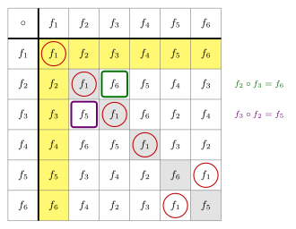
Figure 81: The Cayley table of \(S_3\), the entry in the row of \(f\) and the column of \(g\) being \(f \circ g\). Yellow: the row and column of \(f_1\) repeat the headings, so \(f_1\) is the identity. Red rings: \(f_1\) appears once in every row and column. Four of the rings are on the diagonal, so \(f_1\), \(f_2\), \(f_3\) and \(f_4\) are their own inverses, and the other two show that \(f_5\) and \(f_6\) are inverses of each other. The two boxed entries are mirror images in the main diagonal, shaded grey, and they differ: \(f_2 \circ f_3 = f_6\) but \(f_3 \circ f_2 = f_5\). The table is not symmetric, so the group is not abelian.
Worked: no repeats in a row
Use the group properties to prove that in a Cayley table for a group, the elements in each row are distinct.
A repeat in a row would be the same element \(x\) in two different columns \(b\) and \(c\) of the row of \(a\). So suppose that, and get a contradiction.
Proof (by contradiction). Suppose \((G, *)\) is a group with identity \(e\). Let \(a, b, c, x \in G\) and suppose \(a * b = a * c = x\) with \(b \neq c\). We have
\[\begin{aligned} a * b &= a * c \\ a^{-1} * (a * b) &= a^{-1} * (a * c) && \text{since } a^{-1} \text{ exists in } G \\ (a^{-1} * a) * b &= (a^{-1} * a) * c && \text{associativity} \\ e * b &= e * c && \text{inverses} \\ b &= c && \text{identity} \end{aligned}\]
This contradicts \(b \neq c\). So the elements in each row are distinct. \(\blacksquare\)
A similar argument shows that the elements in each column are distinct.
Every step is licensed by one of the group properties, named at the right, and the proof uses three of the four: inverses, associativity and identity. It is the working of \(2x = 4\), so \(x = 2\), carried out in any group: apply \(a^{-1}\) on the left of both sides and \(a\) cancels. The column version and what the result means for a table are in cayley-tables.
See also
- [groups] — the four properties, abelian groups, and the eight candidates checked one by one
- integers-modulo-n — \(\mathbb{Z}_n\) as a set of equivalence classes, and why any representative can be used
- cayley-tables — reading identity, inverses and commutativity off a table, and why rows and columns have no repeats
- symmetric-group — \(S_n\), the six elements of \(S_3\), and composing them
- composition-of-functions · one-to-one-and-onto-functions — the operation and the elements of \(S_n\)
- 2026-09-22-partial-order-relations — Lecture 25 · 2026-10-06-elementary-properties-of-groups — Lecture 27
- practice-problems — §33, with full worked solutions
Week 10
Lecture 27 — Elementary Properties of Groups
One more group checked from the definition, the functions \(ax + b\) under composition, and then three new ideas: a subgroup, a group sitting inside another under the same operation; powers of an element, including zero and negative powers; and the cyclic subgroup an element generates, which leads to cyclic groups. Pre-work: Video 034 (Elementary Properties of Groups). Subgroups, powers, cyclic subgroups and cyclic groups are collected in subgroups-and-cyclic-groups, the definition of a group and the rules for inverses in [groups], and the classes \([a]\) in integers-modulo-n. How a subgroup shows up in a table is in cayley-tables. The cyclic subgroups of \(\mathbb{Z}_8\) and cyclic groups are also worked in 2026-10-08-definitions-and-examples-of-fields.
Goals
- Become more familiar with groups.
- Understand subgroups and other elementary properties of groups.
- Learn how to work with powers of elements in groups and to generate cyclic subgroups.
A question to keep in mind:
- What does it mean for a group \((G, *)\) to be cyclic? That every element of \(G\) is a power of one single element. The definition is below, after the powers it needs.
A group inside a group
Here is the Cayley table of \((\mathbb{Z}_6, +)\) with its elements listed in an unusual order, the even classes \([0], [2], [4]\) first and then the odd ones \([1], [3], [5]\).
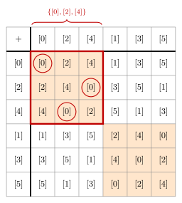
Figure 82: The table of \((\mathbb{Z}_6, +)\) with the even classes listed first. The top-left block, outlined, is a complete table on its own: its headings are \([0], [2], [4]\) and its body uses only \([0], [2], [4]\). So that set is closed under \(+\), it contains the identity \([0]\), and the rings show each element’s inverse inside it: \([0] + [0] = [0]\) and \([2] + [4] = [4] + [2] = [0]\). It is a group in its own right, a subgroup of \(\mathbb{Z}_6\). Shaded cells hold even classes. The bottom-right block is also all even, but its headings are odd, so it is not the table of anything: an odd plus an odd is even.
So \(\{[0], [2], [4]\}\) is a group under the same operation as \(\mathbb{Z}_6\), made of some of its elements. That is what a subgroup is. It is also exactly the set of multiples of \([2]\), \(\{[2], [2] + [2], [2] + [2] + [2]\} = \{[2], [4], [0]\}\), which makes it the cyclic subgroup generated by \([2]\). Listing a subgroup’s elements first, to make it a block, works for any subgroup of any finite group (cayley-tables).
Worked: the functions \(ax + b\) form a group
Show that \((F, \circ)\) is a group, where \(F\) is the set of all functions of the form \(f(x) = ax + b\) where \(a \in \mathbb{R} - \{0\}\) and \(b \in \mathbb{R}\), and \(\circ\) is function composition.
The four properties to check, numbered as in [groups]:
(1) Closure: for all \(g, h \in G\), \(g * h \in G\).
(2) Associativity: for all \(g, h, k \in G\), \((g * h) * k = g * (h * k)\).
(3) Identity: \(\exists e \in G\) such that \(\forall g \in G\), \(e * g = g * e = g\).
(4) Inverses: \(\forall g \in G\), \(\exists g^{-1} \in G\) such that \(g * g^{-1} = g^{-1} * g = e\).
Here \(G\) is \(F\), \(*\) is \(\circ\), and the identity will turn out to be \(I(x) = x\).
An element of \(F\) is a straight-line function with a non-zero slope, and it is pinned down by two numbers: the coefficient \(a \neq 0\) and the constant \(b\). Every check below comes down to the same move. Work out a composite, collect it into the form \((\text{number})\,x + (\text{number})\), and see whether the coefficient of \(x\) is non-zero.
Throughout, let
\[f(x) = ax + b, \qquad g(x) = cx + d, \qquad h(x) = mx + n,\]
where \(a, b, c, d, m, n \in \mathbb{R}\) and \(a, c, m \neq 0\).
(1) Closure. Show that if \(f, g \in F\) then \(f \circ g \in F\).
\[\begin{aligned} (f \circ g)(x) &= f(cx + d) \\ &= a(cx + d) + b \\ &= (ac)\,x + (ad + b). \end{aligned}\]
This is \(Ax + B\) with \(A = ac\) and \(B = ad + b\). Since \(a, b, c, d \in \mathbb{R}\), both \(ac\) and \(ad + b\) are in \(\mathbb{R}\). Since \(a \neq 0\) and \(c \neq 0\), \(ac \neq 0\). So \(f \circ g \in F\), and \(F\) is closed. \(\checkmark\)
(2) Associativity. Show that \((f \circ g) \circ h = f \circ (g \circ h)\). Let \(y = h(x) = mx + n\). Then, using the closure working,
\[\begin{aligned} \big((f \circ g) \circ h\big)(x) &= (f \circ g)(y) = f(cy + d) \\ &= a(cy + d) + b = (ac)\,y + (ad + b) \\ &= (ac)(mx + n) + (ad + b) \\ &= (acm)\,x + (acn + ad + b), \end{aligned}\]
and
\[\begin{aligned} \big(f \circ (g \circ h)\big)(x) &= f\big(g(mx + n)\big) = f\big(c(mx + n) + d\big) \\ &= f\big((cm)\,x + (cn + d)\big) \\ &= a\big((cm)\,x + cn + d\big) + b \\ &= (acm)\,x + (acn + ad + b). \end{aligned}\]
The two agree for every \(x\), so \((f \circ g) \circ h = f \circ (g \circ h)\). \(\checkmark\) Composition of functions is always associative (groups), so this could have been quoted; the algebra confirms it for this family.
(3) Identity. Show that there is an \(I \in F\) with \(f = I \circ f = f \circ I\) for all \(f \in F\). Suppose \(I(x) = ix + j\) is in \(F\) and works, and find \(i\) and \(j\). For \(f = I \circ f\):
\[\begin{aligned} f(x) &= (I \circ f)(x) \\ ax + b &= I(ax + b) \\ &= i(ax + b) + j \\ &= (ia)\,x + (ib + j). \end{aligned}\]
Two straight-line functions are equal for every \(x\) exactly when their coefficients match, so
\[\begin{cases} a = ia & \Rightarrow\ i = 1 \quad (\text{since } a \neq 0), \\ b = ib + j & \Rightarrow\ b = b + j\ \Rightarrow\ j = 0. \end{cases}\]
So \(I(x) = 1x + 0 = x\). It is in \(F\), because its coefficient \(1\) is non-zero, and it satisfies \(f = I \circ f\) for all \(f \in F\). The other side: \((f \circ I)(x) = f(I(x)) = f(x)\), so \(f \circ I = f\). \(F\) has identity \(I(x) = x\). \(\checkmark\)
(4) Inverses. Show that for every \(f \in F\) there is an \(f^{-1} \in F\) with \(f \circ f^{-1} = f^{-1} \circ f = I\). Let \(f(x) = ax + b\) with \(a \neq 0\), and suppose \(g(x) = cx + d\), with \(c \neq 0\), satisfies \(f \circ g = I\). Then
\[\begin{aligned} I(x) &= (f \circ g)(x) \\ x &= f(cx + d) = a(cx + d) + b \\ &= (ac)\,x + (ad + b). \end{aligned}\]
Equating coefficients, with \(x = 1x + 0\) on the left:
\[\left\{\begin{array}{lll} 1 = ac & \Rightarrow\ c = \dfrac1a \in \mathbb{R} - \{0\} & (\text{since } a \neq 0 \text{ and } a \in \mathbb{R}), \\[2mm] 0 = ad + b & \Rightarrow\ d = -\dfrac{b}{a} \in \mathbb{R} & (\text{since } a \neq 0 \text{ and } a, b \in \mathbb{R}). \end{array}\right.\]
So \(g(x) = \frac1a x - \frac{b}{a}\), which is in \(F\). It was found from \(f \circ g = I\) alone, so check the other order:
\[(g \circ f)(x) = g(ax + b) = \frac1a(ax + b) - \frac{b}{a} = x + \frac{b}{a} - \frac{b}{a} = x = I(x).\]
So \(g \circ f = f \circ g = I\), and \(g = f^{-1}\): the inverse of \(f(x) = ax + b\) is \(f^{-1}(x) = \frac1a x - \frac{b}{a}\). \(\checkmark\) For instance \(f(x) = 2x + 6\) has \(f^{-1}(x) = \frac12 x - 3\). “Double, then add 6” is undone by “subtract 6, then halve”.
All four properties hold, so \((F, \circ)\) is a group.
Two remarks:
- Why \(a \neq 0\). With \(a = 0\) the function \(f(x) = b\) is constant. It sends everything to \(b\), so nothing composed with it can give back \(x\), and it has no inverse. Leaving out \(a = 0\) is what makes \(F\) a group, in the same way that leaving out \(0\) turns \((\mathbb{R}, \cdot)\) into the group \((\mathbb{R} - \{0\}, \cdot)\).
- \(F\) is not abelian. In general \(f \circ g = (ac)\,x + (ad + b)\) and \(g \circ f = (ca)\,x + (cb + d)\) have different constants. With \(f(x) = 2x\) and \(g(x) = x + 1\), \((f \circ g)(x) = 2x + 2\) but \((g \circ f)(x) = 2x + 1\). So, like \(S_3\) (symmetric-group), this is a group in which the order of a composition matters.
Subgroups
Definition. If \((G, *)\) is a group and \(H \subseteq G\), then \(H\) is a subgroup of \(G\) if \((H, *)\) is itself a group.
The operation is the same one. To check that \((H, *)\) is a subgroup of \((G, *)\), check three properties:
- closure: for all \(g, h \in H\), \(g * h \in H\);
- identity: the identity is in \(H\);
- inverses: for every \(h \in H\), its inverse is in \(H\).
Associativity is not on the list, because \(H\) inherits it. \((g * h) * k = g * (h * k)\) holds for all \(g, h, k \in G\), so in particular it holds for all \(g, h, k \in H\). \(G\) associative \(\Rightarrow\) \(H\) associative under \(*\). The other three can fail, because each one asks for an element to be in \(H\). More on subgroups, and why the identity of \(H\) has to be the identity of \(G\), is in subgroups-and-cyclic-groups.
Worked: is \(\mathbb{Z}\) a subgroup of \((\mathbb{R}, +)\)?
True or false: \(\mathbb{Z}\) is a subgroup of \((\mathbb{R}, +)\).
True. To prove it, show that the three properties hold for all elements. \(\mathbb{Z} \subseteq \mathbb{R}\). Let \(a, b \in \mathbb{Z}\).
- Closure \(\checkmark\). \(a + b \in \mathbb{Z}\), so \(\mathbb{Z}\) is closed under \(+\).
- Identity \(\checkmark\). \(0 \in \mathbb{Z}\), since \(a + 0 = 0 + a = a\).
- Inverses \(\checkmark\). \(-a \in \mathbb{Z}\), and \(a + (-a) = (-a) + a = 0\).
Associativity comes free from \((\mathbb{R}, +)\), so \(\mathbb{Z}\) is a subgroup of \((\mathbb{R}, +)\).
Worked: is \(\mathbb{R} - \{0\}\) a subgroup of \((\mathbb{R}, +)\)?
True or false: \(\mathbb{R} - \{0\}\) is a subgroup of \((\mathbb{R}, +)\).
False. To disprove it, one property failing for specific elements is enough: a counterexample to one property.
- Closure \(\times\). Let \(a \in \mathbb{R} - \{0\}\). Then \(-a \in \mathbb{R} - \{0\}\) as well, but \(a + (-a) = 0 \notin \mathbb{R} - \{0\}\). For example \(1 + (-1) = 0\). So the set is not closed under \(+\).
- Identity \(\times\). The identity of \((\mathbb{R}, +)\) is \(0\), and it has been removed. No other element could stand in for it, since \(e + a = a\) forces \(e = 0\).
- Inverses. There is nothing to check against: an inverse is defined as an element that combines with \(a\) to give the identity, and there is no identity.
The same set is a group under multiplication, \((\mathbb{R} - \{0\}, \cdot)\) (groups). But a subgroup must use the operation of the group it sits in, and under \(+\) it fails.
Powers of an element
If \((G, *)\) is a group and \(a \in G\), then \(a^i\) is defined for each \(i \in \mathbb{Z}\) as follows:
\(a^0 = e\), where \(e\) is the identity of \(G\);
\(a^i = \underbrace{a * a * \cdots * a}_{i \text{ times}}\) for each \(i \in \mathbb{Z}^{+}\);
\(a^{-i} = \underbrace{a^{-1} * a^{-1} * \cdots * a^{-1}}_{i \text{ times}}\) for each \(i \in \mathbb{Z}^{+}\).
So \(a^1 = a\), \(a^2 = a * a\), \(a^3 = a * a * a\), and so on. A negative power is a power of the inverse: \(a^{-1}\), one copy of the inverse, is the inverse of \(a\) under \(*\), exactly as before, and \(a^{-2} = a^{-1} * a^{-1}\).
The power notation is used for any operation \(*\), even if that operation is addition. Be careful with it.
- In \((\mathbb{Z}_{12}, +)\), \(3^2 = 3 + 3 = 6\). It is not \(9\).
- In \((\mathbb{Z}, +)\), \(a^2 = a + a\), and \(a^{-1} = -a\), because \(a^{-1} + a = 0\).
Two laws. For all \(g \in G\):
\[g^i * g^j = g^{i + j}, \qquad\text{because}\qquad \underbrace{g * g * \cdots * g}_{i \text{ times}} * \underbrace{g * g * \cdots * g}_{j \text{ times}} \text{ is } i + j \text{ copies of } g,\]
and
\[\underbrace{g * g * \cdots * g}_{i \text{ times}} * \underbrace{g^{-1} * g^{-1} * \cdots * g^{-1}}_{i \text{ times}} = e,\]
because the \(g\) and the \(g^{-1}\) that meet in the middle combine to \(e\), which drops out, and then the next pair meet, until nothing is left. So
\[(g^i)^{-1} = g^{-i}, \qquad g^i * g^{-i} = g^{i - i} = g^0 = e, \qquad g^{-i} * g^i = g^{-i + i} = g^0 = e.\]
The powers of a group element follow the same exponent rules as powers of a number. The laws for exponents of mixed sign, and a picture of the powers as a line or a loop, are in subgroups-and-cyclic-groups.
Worked: \([3]^4\) and \([3]^{-4}\) in \(\mathbb{Z}_7 - \{[0]\}\)
Calculate \([3]^4\) and \([3]^{-4}\) in the group \((\mathbb{Z}_7 - \{[0]\}, \cdot)\).
Here \([3] = \{a \in \mathbb{Z} : a \equiv 3 \pmod 7\}\), the operation is multiplication of classes, and the identity is \([1]\).
\([3]^4\). Multiply, reducing mod 7 as soon as a product passes 6:
\[[3]^4 = [3] \cdot [3] \cdot [3] \cdot [3] = [9] \cdot [9] = [2] \cdot [2] = \mathbf{[4]}.\]
\([3]^{-4}\). By definition \([3]^{-4} = ([3]^{-1})^4\), and by the second law it is also \(([3]^4)^{-1}\). The second is quicker here, since \([3]^4\) is already known:
\[[3]^{-4} = ([3]^{-1})^4 = ([3]^4)^{-1} = [4]^{-1} = \mathbf{[2]},\]
because \([4] \cdot [2] = [8] = [1]\), that is, \(4 \cdot 2 \equiv 1 \pmod 7\).
Check by the other route. \([3]^{-1} = [5]\), since \([3] \cdot [5] = [15] = [1]\). Then \([3]^{-4} = [5]^4 = [25] \cdot [25] = [4] \cdot [4] = [16] = [2]\). The same. And \([3]^4 \cdot [3]^{-4} = [4] \cdot [2] = [1] = [3]^0\), as the first law says it must be. Both inverses can also be read off the table of this group (2026-09-24-definitions-and-examples-of-groups).
Cyclic subgroups
If \((G, *)\) is a group and \(a \in G\), then \[\langle a \rangle = \{a^i : i \in \mathbb{Z}\}\] is a subgroup of \(G\), and is called the cyclic subgroup of \(G\) generated by \(a\).
\(\langle a \rangle\) is every power of \(a\): positive, zero and negative. It is what any subgroup \(S\) containing \(a\) is forced to contain:
- \(a \in S\), so by closure \(a^2, a^3, a^4, \ldots \in S\);
- by identity \(a^0 = e \in S\), and by inverses \(a^{-1} \in S\), so by closure again \(a^{-2}, a^{-3}, a^{-4}, \ldots \in S\).
And the powers are already a subgroup, by the two laws: closure from \(a^i * a^j = a^{i+j}\), the identity \(a^0\), inverses \((a^i)^{-1} = a^{-i}\). So \(\langle a \rangle\) is the smallest subgroup that contains \(a\).
In a finite group, list the positive powers \(a^1, a^2, a^3, \ldots\) until the list comes back to where it started. After that it only repeats, and the negative powers turn out to be in the list already (subgroups-and-cyclic-groups).
Worked: \(\langle 3 \rangle\) in \(\mathbb{Z}_{11} - \{[0]\}\)
Determine \(\langle 3 \rangle\) in the group \((\mathbb{Z}_{11} - \{[0]\}, \cdot)\).
Each power is the previous one times \([3]\), reduced mod 11:
\[\begin{aligned} [3]^1 &= [3] \\ [3]^2 &= [3] \cdot [3] = [9] \\ [3]^3 &= [3]^2 \cdot [3] = [9] \cdot [3] = [27] = [22 + 5] = [5] \\ [3]^4 &= [3]^3 \cdot [3] = [5] \cdot [3] = [15] = [11 + 4] = [4] \\ [3]^5 &= [3]^4 \cdot [3] = [4] \cdot [3] = [12] = [1] \\ [3]^6 &= [3]^5 \cdot [3] = [1] \cdot [3] = [3] \end{aligned}\]
\([3]^6\) is back to the start, so every element of \(\langle 3 \rangle\) has been found: \([3]^7 = [9]\), \([3]^8 = [5]\), and so on round again. Once it is clear which group is meant, the square brackets are optional:
\[\langle 3 \rangle = \{3, 3^2, 3^3, \ldots\} = \{3, 9, 5, 4, 1\}.\]
The negative powers add nothing. \([3]^5 = [1]\) gives \([3]^4 \cdot [3] = [1]\), so \([3]^{-1} = [3]^4 = [4]\) (check: \([3] \cdot [4] = [12] = [1]\)). Multiplying by \([3]^{-1}\) walks round the same loop backwards, so \([3]^{-1}, [3]^{-2}, \ldots\) are \([4], [5], [9], [3], [1], \ldots\), all already listed.
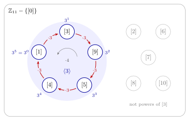
Figure 83: The powers of \([3]\) in \(\mathbb{Z}_{11} - {[0]}\). Each arrow multiplies by \([3]\). Starting from \([3]\) the powers run \([3], [9], [5], [4], [1]\), and since \([3]^5 = [1]\) the next step is back at \([3]\), so the powers go round a loop of five and \(\langle 3 \rangle = {1, 3, 4, 5, 9}\). Going round backwards is multiplying by \([3]^{-1} = [4]\), which gives the negative powers and stays on the same loop. The other five elements of the group are not powers of \([3]\), so \(\langle 3 \rangle\) is a subgroup, not the whole group.
\(\langle 3 \rangle\) has 5 of the group’s 10 elements, so \(3\) does not generate the whole group. Another element does: the powers of \(2\) are all ten elements (practice-problems, Q4).
Worked: all the cyclic subgroups of \((\mathbb{Z}_8, +)\)
Determine all the cyclic subgroups of \((\mathbb{Z}_8, +)\).
\(\mathbb{Z}_8 = \{0, 1, 2, 3, 4, 5, 6, 7\}\), writing the classes without brackets, and any representative names its class, so \(9 = 1\) and \(8 = 0\). The operation is \(+\), so a power is a repeated sum: \(2^3 = 2 + 2 + 2 = 6\). One cyclic subgroup for each element, starting with the identity:
\[\begin{aligned} \langle 0 \rangle &= \{0\} \\ \langle 1 \rangle &= \{1, 2, 3, 4, 5, 6, 7, 8 = 0\} = \mathbb{Z}_8 \\ \langle 2 \rangle &= \{2^n : n \in \mathbb{Z}\} = \{2^1, 2^2, 2^3, 2^4, \ldots\} = \{2, 4, 6, 0\} \\ \langle 3 \rangle &= \{3, 6, 9 = 1, 4, 7, 10 = 2, 5, 0\} = \mathbb{Z}_8 \\ \langle 4 \rangle &= \{4, 8 = 0\} = \{0, 4\} \end{aligned}\]
Each list stops at \(0\), the identity, because the next power is back at the start. The last three need no more work, because \(5 = -3\), \(6 = -2\) and \(7 = -1\) are inverses of elements already done:
\[\langle 5 \rangle = \langle 3^{-1} \rangle = \mathbb{Z}_8, \qquad \langle 6 \rangle = \langle 2^{-1} \rangle = \{0, 2, 4, 6\}, \qquad \langle 7 \rangle = \langle 1^{-1} \rangle = \mathbb{Z}_8.\]
Two rules were used:
- \(\langle \text{identity} \rangle = \{\text{identity}\}\). Every power of \(e\) is \(e\).
- \(\langle a \rangle = \langle a^{-1} \rangle\). The powers of \(a^{-1}\) are \((a^{-1})^i = a^{-i}\), the powers of \(a\) in the opposite order, so they make the same set. Directly: \(\langle 5 \rangle = \{5, 10 = 2, 15 = 7, 20 = 4, 25 = 1, 30 = 6, 35 = 3, 40 = 0\}\), which is \(\langle 3 \rangle\) listed backwards.
So \((\mathbb{Z}_8, +)\) has eight elements but only four different cyclic subgroups, and each one sits inside the next:
\[\{0\} \ \subset\ \{0, 4\} \ \subset\ \{0, 2, 4, 6\} \ \subset\ \mathbb{Z}_8.\]
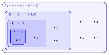
Figure 84: The four cyclic subgroups of \((\mathbb{Z}_8, +)\), each drawn inside the next. Every element generates exactly the smallest region it sits in: \(0\) generates only \({0}\), \(4\) generates \({0, 4}\), \(2\) and \(6\) generate \({0, 2, 4, 6}\), and the four odd elements \(1, 3, 5, 7\) each generate all of \(\mathbb{Z}_8\). Elements that are inverses of each other, such as \(2\) and \(6\), always land in the same region, because \(\langle a \rangle = \langle a^{-1} \rangle\).
Four of the eight elements, \(1, 3, 5, 7\), generate the whole of \(\mathbb{Z}_8\). That makes \(\mathbb{Z}_8\) a cyclic group.
Cyclic groups
The group \((G, *)\) is cyclic if there exists an \(a \in G\) such that \(\langle a \rangle = G\).
That answers the question in the goals: a group is cyclic when every one of its elements is a power of a single element \(a\), called a generator. So far:
- \(\mathbb{Z}_8\) is cyclic: \(\langle 1 \rangle = \langle 3 \rangle = \langle 5 \rangle = \langle 7 \rangle = \mathbb{Z}_8\).
- \(\mathbb{Z}_6\) is cyclic, generated by \([1]\), since \([1], [1] + [1], \ldots\) runs through all six classes. Its subgroup \(\{[0], [2], [4]\} = \langle [2] \rangle\), from the table above, is a cyclic subgroup that is not the whole group.
- \(\mathbb{Z}_{11} - \{[0]\}\) is cyclic, generated by \(2\), even though \(3\) is not a generator. One generator is all it takes.
How to prove a group is cyclic, and how to prove it is not, is in subgroups-and-cyclic-groups.
Worked: which of these groups are cyclic?
Which of the following groups are cyclic? \((\mathbb{Z}_{10}, +)\), \(\ (\mathbb{Z}_5 - \{[0]\}, \cdot)\), \(\ (\mathbb{Z}, +)\), \(\ (\mathbb{Q}, +)\).
| Group | Cyclic? | Generated by |
|---|---|---|
| \((\mathbb{Z}_{10}, +)\) | \(\checkmark\) yes | \(1\) |
| \((\mathbb{Z}_5 - \{[0]\}, \cdot)\) | \(\checkmark\) yes | \(2\) |
| \((\mathbb{Z}, +)\) | \(\checkmark\) yes | \(1\) |
| \((\mathbb{Q}, +)\) | \(\times\) no | nothing |
\((\mathbb{Z}_{10}, +)\). \(1^n = 1 + 1 + \cdots + 1 = n\), so the powers of \(1\) are \(1, 2, \ldots, 9, 10 = 0\): every element. \(\mathbb{Z}_{10} = \langle 1 \rangle\).
\((\mathbb{Z}_5 - \{[0]\}, \cdot)\). The set is \(\{1, 2, 3, 4\}\). The identity is no use, since \(\langle 1 \rangle = \{1\}\). Try \(2\): \(2^1 = 2\), \(2^2 = 4\), \(2^3 = 8 = 3\), \(2^4 = 16 = 1\). So \(\langle 2 \rangle = \{2, 4, 3, 1\}\), the whole group. (\(3\) is also a generator; \(4\) is not, since \(\langle 4 \rangle = \{4, 1\}\).)
\((\mathbb{Z}, +)\). Here the negative powers are essential:
\[\langle 1 \rangle = \{1^n : n \in \mathbb{Z}\} = \{\ldots, 1^{-2}, 1^{-1}, 1^0, 1^1, 1^2, \ldots\} = \{\ldots, -2, -1, 0, 1, 2, \ldots\} = \mathbb{Z}.\]
The positive powers of \(1\) give only \(1, 2, 3, \ldots\). The zero power is the identity \(0\), and \(1^{-n} = (-1) + \cdots + (-1) = -n\) fills in the negatives.
\((\mathbb{Q}, +)\). Not cyclic. That means showing that no \(a \in \mathbb{Q}\) generates it. In \((\mathbb{Q}, +)\) the powers of \(a\) are its integer multiples, so \(\langle a \rangle = \{na : n \in \mathbb{Z}\}\).
- If \(a = 0\), then \(\langle a \rangle = \{0\} \neq \mathbb{Q}\).
- If \(a = \frac{p}{q} \neq 0\), where \(p, q \in \mathbb{Z}\) and \(q \neq 0\), then \(\frac{p}{2q} = \frac{a}{2} \in \mathbb{Q}\). But \(\frac{p}{2q} = n \cdot \frac{p}{q}\) would need \(n = \frac12\), which is not an integer. So \(\frac{p}{2q} \notin \left\langle \frac{p}{q} \right\rangle\), and \(\langle a \rangle \neq \mathbb{Q}\).
Either way \(\langle a \rangle \neq \mathbb{Q}\), so \((\mathbb{Q}, +)\) is not cyclic. The multiples of any one rational are evenly spaced with gaps, and half of it falls in the first gap. A picture is in subgroups-and-cyclic-groups.
Worked: \(\mathbb{Z}_2 \times \mathbb{Z}_3\) is cyclic
Consider the group \((\mathbb{Z}_2 \times \mathbb{Z}_3, +)\) where \((a, b) + (c, d) = \big((a + c) \bmod 2,\ (b + d) \bmod 3\big)\). Show that this group is cyclic.
The group has \(2 \cdot 3 = 6\) elements, the pairs \((a, b)\) with \(a \in \{0, 1\}\) and \(b \in \{0, 1, 2\}\), and its identity is \((0, 0)\). Take \((a, b) = (1, 1)\) and add it on each time:
\[\begin{aligned} (1,1)^1 &= (1, 1) \\ (1,1)^2 &= (1,1) + (1,1) = (2 \bmod 2,\ 2 \bmod 3) = (0, 2) \\ (1,1)^3 &= (1,1)^2 + (1,1) = (0,2) + (1,1) = (1, 0) \\ (1,1)^4 &= (1,0) + (1,1) = (0, 1) \\ (1,1)^5 &= (0,1) + (1,1) = (1, 2) \\ (1,1)^6 &= (1,2) + (1,1) = (0, 0) \end{aligned}\]
The six powers are six different elements, so they are the whole group: \(\mathbb{Z}_2 \times \mathbb{Z}_3 = \langle (1, 1) \rangle\), and the group is cyclic. \(\blacksquare\)
It works because the first coordinate comes back to \(0\) every 2 steps and the second every 3 steps, and the two are back at \(0\) together for the first time at step 6. Not every element generates: \((0, 1)\) gives only \(\{(0,0), (0,1), (0,2)\}\) and \((1, 0)\) only \(\{(0,0), (1,0)\}\). These three are drawn in subgroups-and-cyclic-groups.
See also
- subgroups-and-cyclic-groups — subgroups, powers and the power laws, \(\langle a \rangle\), and cyclic groups, with more examples
- [groups] — the four properties, and the elementary properties: unique identity and inverses, the inverse of a product
- cayley-tables — reading a subgroup off a table by listing its elements first
- integers-modulo-n — \(\mathbb{Z}_n\) and \(\mathbb{Z}_n - \{[0]\}\), the groups most of the examples live in
- composition-of-functions · inverse-functions — the operation and the inverses in the group \((F, \circ)\)
- symmetric-group — the cyclic subgroups of \(S_3\), which is not cyclic
- 2026-09-24-definitions-and-examples-of-groups — Lecture 26 · 2026-10-08-definitions-and-examples-of-fields — Lecture 28
- practice-problems — §34, with full worked solutions
Lecture 28 — Definitions and Examples of Fields
The cyclic subgroups of \(\mathbb{Z}_8\) and which groups are cyclic, then fields: a set with two operations that is an abelian group under each of them, joined by the distributive laws. Which of \(\mathbb{Z}\), \(\mathbb{Z}_4\), \(\mathbb{Z}_7\) and \(\mathbb{Z}_{15}\) are fields, and how to solve a linear equation in \(\mathbb{Z}_{11}\) and \(\mathbb{Z}_{17}\). Pre-work: Video 036 (Definitions and Examples of Fields). Fields are collected in [fields], cyclic subgroups and cyclic groups in subgroups-and-cyclic-groups, and \(\mathbb{Z}_p\) and multiplicative inverses mod \(p\) in integers-modulo-n. The group definition everything here leans on is in [groups].
Goals
- Review the concepts of groups, abelian groups, subgroups and cyclic subgroups.
- Become familiar with calculations in fields.
- Learn how to solve equations in fields.
The four terms in the first goal, in one line each:
- Group. A set with a binary operation, \((G, *)\), satisfying closure, associativity, identity and inverses (groups).
- Abelian. \(a * b = b * a\) for all \(a, b \in G\).
- Subgroup. A subset of \(G\) that is a group under the same operation (subgroups-and-cyclic-groups).
- Cyclic subgroup. \(\langle a \rangle = \{a^n : n \in \mathbb{Z}\}\), every power of \(a\): positive, zero and negative.
Cyclic subgroups
If \((G, *)\) is a group and \(a \in G\), then \[\langle a \rangle = \{a^i : i \in \mathbb{Z}\}\] is a subgroup of \(G\), and is called the cyclic subgroup of \(G\) generated by \(a\).
The powers are taken with the group’s own operation: \(a^2 = a * a\), \(a^0 = e\), and \(a^{-i} = (a^{-1})^i\). In an additive group such as \((\mathbb{Z}_n, +)\) a “power” is a repeated sum, so \([a]^i = [ia]\), and \(\langle [a] \rangle\) is the set of multiples of \([a]\). The full treatment is in subgroups-and-cyclic-groups.
Worked: the cyclic subgroups of \((\mathbb{Z}_8, +)\)
Determine all the cyclic subgroups of \((\mathbb{Z}_8, +)\).
\(\mathbb{Z}_8 = \{[0], [1], [2], [3], [4], [5], [6], [7]\}\), so there are eight elements to try. For each, keep adding \([a]\) until the sum comes back to \([0]\); after that the list repeats. The negative powers add nothing new: if \(k\) copies of \([a]\) make \([0]\), then \([a]^{-1} = [a]^{k-1}\), so every negative power is already one of the positive ones.
\[\begin{aligned} \langle [0] \rangle &= \{[0]\} \\ \langle [1] \rangle &= \{[1], [2], [3], [4], [5], [6], [7], [8] = [0]\} = \mathbb{Z}_8 \\ \langle [2] \rangle &= \{[2], [4], [6], [8] = [0]\} = \{[0], [2], [4], [6]\} \\ \langle [3] \rangle &= \{[3], [6], [9] = [1], [4], [7], [10] = [2], [5], [8] = [0]\} = \mathbb{Z}_8 \\ \langle [4] \rangle &= \{[4], [8] = [0]\} = \{[0], [4]\} \end{aligned}\]
The other three, \(\langle [5] \rangle\), \(\langle [6] \rangle\) and \(\langle [7] \rangle\), need no new work, because of two rules that hold in any group:
- \(\langle e \rangle = \{e\}\). Every power of the identity is the identity. That is \(\langle [0] \rangle = \{[0]\}\) above.
- \(\langle a \rangle = \langle a^{-1} \rangle\). The powers of \(a^{-1}\) are \((a^{-1})^i = a^{-i}\), and as \(i\) runs through \(\mathbb{Z}\) so does \(-i\). The two lists are the same powers taken in the opposite order.
In \((\mathbb{Z}_8, +)\) the inverse of \([a]\) is \([-a] = [8 - a]\), so \([5] = [3]^{-1}\), \([6] = [2]^{-1}\) and \([7] = [1]^{-1}\):
\[\langle [5] \rangle = \langle [3] \rangle = \mathbb{Z}_8, \qquad \langle [6] \rangle = \langle [2] \rangle = \{[0], [2], [4], [6]\}, \qquad \langle [7] \rangle = \langle [1] \rangle = \mathbb{Z}_8.\]
So \(\mathbb{Z}_8\) has four distinct cyclic subgroups, \(\{[0]\}\), \(\{[0], [4]\}\), \(\{[0], [2], [4], [6]\}\) and \(\mathbb{Z}_8\) itself, and
\[\langle [1] \rangle = \langle [3] \rangle = \langle [5] \rangle = \langle [7] \rangle = \mathbb{Z}_8.\]
The four elements that reach everything are the odd ones. An even step from \([0]\) only ever lands on even classes. The four subgroups sit inside one another, \(\{[0]\} \subseteq \{[0], [4]\} \subseteq \{[0], [2], [4], [6]\} \subseteq \mathbb{Z}_8\), as drawn in 2026-10-06-elementary-properties-of-groups.
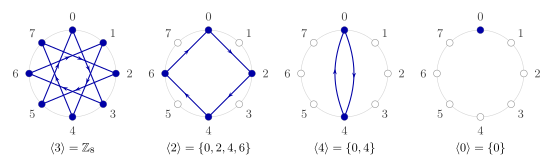
Figure 85: Each cyclic subgroup of \(\mathbb{Z}_8\) as a walk round the eight classes, written without brackets, taking steps of \(a\) from 0 until the walk closes. Filled dots are the classes reached, and they make up \(\langle a \rangle\). Steps of 3 visit all eight classes before returning, so \(\langle 3 \rangle = \mathbb{Z}_8\). Steps of 2 visit only the even classes, steps of 4 only 0 and 4, and steps of 0 never leave 0. Steps of 5, 6 and 7 trace the same walks as steps of 3, 2 and 1, run backwards, which is why \(\langle a \rangle = \langle a^{-1} \rangle\).
Cyclic groups
The group \((G, *)\) is cyclic if there exists an \(a \in G\) such that \(\langle a \rangle = G\).
Such an \(a\) is a generator of \(G\). Every element of a cyclic group is a power of the one element \(a\). By the last section, \((\mathbb{Z}_8, +)\) is cyclic, with four generators. More on cyclic groups is in subgroups-and-cyclic-groups.
Worked: which of these groups are cyclic?
Which of the following groups are cyclic? \((\mathbb{Z}_{10}, +)\), \(\ (\mathbb{Z}_5 - \{[0]\}, \cdot)\), \(\ (\mathbb{Z}, +)\), \(\ (\mathbb{Q}, +)\).
| Group | Cyclic? | Generator |
|---|---|---|
| \((\mathbb{Z}_{10}, +)\) | yes | \([1]\) |
| \((\mathbb{Z}_5 - \{[0]\}, \cdot)\) | yes | \([2]\) |
| \((\mathbb{Z}, +)\) | yes | \(1\) |
| \((\mathbb{Q}, +)\) | no | none |
\((\mathbb{Z}_{10}, +)\). The multiples of \([1]\) are \([1], [2], \dots, [9], [10] = [0]\), all ten classes. So \(\mathbb{Z}_{10} = \langle [1] \rangle\).
\((\mathbb{Z}_5 - \{[0]\}, \cdot)\). The set is \(\{[1], [2], [3], [4]\}\) and the operation is multiplication, so here powers really are powers. \(\langle [1] \rangle = \{[1]\}\), since \([1]\) is the identity. Trying \([2]\):
\[[2]^1 = [2], \quad [2]^2 = [4], \quad [2]^3 = [8] = [3], \quad [2]^4 = [16] = [1].\]
So \(\langle [2] \rangle = \{[2], [4], [3], [1]\} = \mathbb{Z}_5 - \{[0]\}\), and the group is cyclic. A generator only has to exist; \([1]\) failing does not matter.
\((\mathbb{Z}, +)\). In additive notation \(1^n\) is \(n\) copies of 1 added together, \(1^0 = 0\), and \(1^{-1} = -1\). So
\[\langle 1 \rangle = \{1^n : n \in \mathbb{Z}\} = \{\dots, 1^{-2}, 1^{-1}, 1^0, 1^1, 1^2, \dots\} = \{\dots, -2, -1, 0, 1, 2, \dots\} = \mathbb{Z}.\]
An infinite group can be cyclic.
\((\mathbb{Q}, +)\). To show no generator exists, take an arbitrary rational \(r\) and find a rational that is not in \(\langle r \rangle\). In \((\mathbb{Q}, +)\), \(\langle r \rangle = \{kr : k \in \mathbb{Z}\}\), the integer multiples of \(r\).
- If \(r = 0\), then \(\langle 0 \rangle = \{0\}\), which is not \(\mathbb{Q}\).
- If \(r \neq 0\), write \(r = \frac{p}{q}\) with \(p, q \in \mathbb{Z}\), \(q \neq 0\). Then \(\frac{p}{2q} = \frac{r}{2}\) is rational. If it were in \(\langle r \rangle\) there would be a \(k \in \mathbb{Z}\) with \(\frac{r}{2} = kr\), and dividing by \(r \neq 0\) gives \(k = \frac12\), which is not an integer. So \(\frac{p}{2q} \notin \langle \frac{p}{q} \rangle\).
Either way \(\langle r \rangle \neq \mathbb{Q}\), so \((\mathbb{Q}, +)\) is not cyclic. The case \(r = 0\) has to be split off because \(\frac{0}{2q} = 0\) is in \(\langle 0 \rangle\). On the number line, \(\langle r \rangle\) is a row of equally spaced points, and \(\frac{r}{2}\) sits in the first gap (subgroups-and-cyclic-groups draws it).
Worked: \(\mathbb{Z}_2 \times \mathbb{Z}_3\) is cyclic
Consider the group \((\mathbb{Z}_2 \times \mathbb{Z}_3, +)\) where \((a, b) + (c, d) = \big((a + c) \bmod 2,\ (b + d) \bmod 3\big)\). Show that this group is cyclic.
The elements are the six pairs \((a, b)\) with \(a \in \{0, 1\}\) and \(b \in \{0, 1, 2\}\), and the operation adds each coordinate in its own modulus. Try \((a, b) = (1, 1)\), adding \((1, 1)\) each time:
\[\begin{aligned} (1,1)^1 &= (1, 1) \\ (1,1)^2 &= (1,1) + (1,1) = (2 \bmod 2,\ 2 \bmod 3) = (0, 2) \\ (1,1)^3 &= (1,1)^2 + (1,1) = (0,2) + (1,1) = (1 \bmod 2,\ 3 \bmod 3) = (1, 0) \\ (1,1)^4 &= (1,0) + (1,1) = (0, 1) \\ (1,1)^5 &= (0,1) + (1,1) = (1, 2) \\ (1,1)^6 &= (1,2) + (1,1) = (0, 0) \end{aligned}\]
The six powers are six different pairs, so they are all of \(\mathbb{Z}_2 \times \mathbb{Z}_3\), and
\[\mathbb{Z}_2 \times \mathbb{Z}_3 = \langle (1, 1) \rangle. \qquad /\!/\]
Not every element works. \((1, 0)\) only reaches \((1, 0)\) and \((0, 0)\), and \((0, 1)\) only reaches the three pairs with first coordinate 0. \((1, 1)\) works because its first coordinate cycles with period 2 and its second with period 3, and the two are not back at \((0, 0)\) together until the sixth step. The three cyclic subgroups are drawn side by side in subgroups-and-cyclic-groups.
The definition of a field
Definition. A field \((F, +, \cdot)\) is a set \(F\) with two binary operations \(+\) and \(\cdot\) such that
(1) \((F, +)\) is an abelian group;
(2) \((F - \{0\}, \cdot)\) is an abelian group, where \(0\) is the identity of \((F, +)\); and
(3) for all \(f, g, h \in F\), \(\ f \cdot (g + h) = (f \cdot g) + (f \cdot h)\) and \((f + g) \cdot h = (f \cdot h) + (g \cdot h)\).
Condition (3) is the pair of distributive laws. They are the only condition that involves both operations at once; without them \(+\) and \(\cdot\) would be two unrelated groups that happen to share a set.
Condition (1) is five checks: closure, associativity, identity and inverses for \(+\), and commutativity to make it abelian. Condition (2) is the same five for \(\cdot\), on the smaller set \(F - \{0\}\). The “0” there means the additive identity, whatever it is called in \(F\); in \(\mathbb{Z}_n\) it is \([0]\). Why it has to be removed, and a picture of the two groups, are in fields.
Fields already in use
\((\mathbb{R}, +, \cdot)\) and \((\mathbb{Q}, +, \cdot)\) are fields. Arithmetic in them uses both kinds of inverse:
- subtraction is adding an additive inverse, \(a - b = a + (-b)\);
- division is multiplying by a multiplicative inverse, \(a \div b = a \cdot b^{-1}\) for \(b \neq 0\).
Example. Solve \(2x + 3 = 8\) in \(\mathbb{R}\). Add \(-3\) to both sides to get \(2x = 5\), then multiply both sides by \(2^{-1} = \frac12\) to get \(x = \frac52\).
Those two steps are all that solving a linear equation needs, and the field axioms are what guarantee they can be done. The same two steps work in any field, including those where \(-3\) and \(2^{-1}\) are classes mod \(p\).
Worked: is \((\mathbb{Z}_4, +, \cdot)\) a field?
Is \((\mathbb{Z}_4, +, \cdot)\) a field?
No. Condition (1) holds but condition (2) fails.
(1) \((\mathbb{Z}_4, +)\) is an abelian group with identity \([0]\). From the table: closure (only \([0], \dots, [3]\) appear), associativity (inherited from addition of integers), identity \([0]\) (its row and column repeat the headings), inverses (\([0]\) is in every row: \(-[1] = [3]\), \(-[2] = [2]\), \(-[3] = [1]\)), and commutative (the table is symmetric about its diagonal).
| \(+\) | \([0]\) | \([1]\) | \([2]\) | \([3]\) |
|---|---|---|---|---|
| \(\mathbf{[0]}\) | \([0]\) | \([1]\) | \([2]\) | \([3]\) |
| \(\mathbf{[1]}\) | \([1]\) | \([2]\) | \([3]\) | \([0]\) |
| \(\mathbf{[2]}\) | \([2]\) | \([3]\) | \([0]\) | \([1]\) |
| \(\mathbf{[3]}\) | \([3]\) | \([0]\) | \([1]\) | \([2]\) |
(2) \((\mathbb{Z}_4 - \{[0]\}, \cdot)\) is not a group. The set is \(\{[1], [2], [3]\}\):
| \(\cdot\) | \([1]\) | \([2]\) | \([3]\) |
|---|---|---|---|
| \(\mathbf{[1]}\) | \([1]\) | \([2]\) | \([3]\) |
| \(\mathbf{[2]}\) | \([2]\) | \(\mathbf{[0]}\) | \([2]\) |
| \(\mathbf{[3]}\) | \([3]\) | \([2]\) | \([1]\) |
\([2] \cdot [2] = [4] = [0]\), and \([0] \notin \mathbb{Z}_4 - \{[0]\}\). Closure fails. Two non-zero classes multiply to zero. The same row shows a second failure: the row of \([2]\) has no \([1]\) in it, so \([2]\) has no multiplicative inverse either.
Worked: which of these is a field?
Two rules to use:
- \((\mathbb{Z}_n, +)\) is a group for every \(n \in \mathbb{Z}^{+}\) (integers-modulo-n). It is abelian, so condition (1) always holds for \(\mathbb{Z}_n\).
- \((\mathbb{Z}_p, +, \cdot)\) is a field when \(p\) is prime. Why, and why a composite \(n\) never works, is in fields.
Which of the following is a field? (a) \((\mathbb{Z}, +, \cdot)\) \(\quad\) (b) \((\mathbb{Z}_7, +, \cdot)\) \(\quad\) (c) \((\mathbb{Z}_{15}, +, \cdot)\)
(a) \((\mathbb{Z}, +, \cdot)\): not a field.
- \((\mathbb{Z}, +)\) is an abelian group with identity 0. \(\checkmark\)
- \((\mathbb{Z} - \{0\}, \cdot)\) is not a group, because 2 has no inverse: the identity is 1, and \(2 \cdot y = 1\) needs \(y = \frac12 \notin \mathbb{Z}\). \(\times\)
So \((\mathbb{Z}, +, \cdot)\) is not a field. This is where the second step of solving an equation breaks down in \(\mathbb{Z}\): there is no \(2^{-1}\) to multiply \(2x = 5\) by, and indeed no integer \(x\) has \(2x = 5\).
(b) \((\mathbb{Z}_7, +, \cdot)\): a field, since 7 is prime. Checking each condition directly:
- \((\mathbb{Z}_7, +)\) is an abelian group with identity \([0]\), by the first rule. \(\checkmark\)
- \((\mathbb{Z}_7 - \{[0]\}, \cdot)\) is the abelian group whose table is worked in 2026-09-24-definitions-and-examples-of-groups. Its inverses are \([1]^{-1} = [1]\), \([2]^{-1} = [4]\), \([3]^{-1} = [5]\), \([6]^{-1} = [6]\). \(\checkmark\)
- The distributive laws are inherited from the integers: \([a] \cdot ([b] + [c]) = [a(b + c)] = [ab + ac] = [a][b] + [a][c]\), and the other law follows the same way. \(\checkmark\)
(c) \((\mathbb{Z}_{15}, +, \cdot)\): not a field.
- \((\mathbb{Z}_{15}, +)\) is an abelian group with identity \([0]\). \(\checkmark\)
- \((\mathbb{Z}_{15} - \{[0]\}, \cdot)\) is not a group: \([3] \cdot [5] = [15] = [0]\), which is not in the set, so closure fails. \(\times\)
So \((\mathbb{Z}_{15}, +, \cdot)\) is not a field. The factorisation \(15 = 3 \cdot 5\) is exactly what produces the two non-zero classes with product \([0]\).
Solving equations in a field
In a field, a linear equation is solved exactly as in \(\mathbb{R}\): add the additive inverse of the constant to both sides, then multiply both sides by the multiplicative inverse of the coefficient. In \(\mathbb{Z}_p\) both inverses are classes, and the multiplicative one has to be found. The general method, with a picture, is in fields.
Worked: linear equations in \(\mathbb{Z}_{11}\) and \(\mathbb{Z}_{17}\)
(a) Solve the equation \(2x + 3 = 8\) in the field \((\mathbb{Z}_{11}, +, \cdot)\). Hence determine the smallest positive integer \(y\) such that \(2y + 3 \equiv 8 \pmod{11}\).
(b) Solve the equation \(10x + 9 = 6\) in the field \((\mathbb{Z}_{17}, +, \cdot)\). Hence determine the smallest positive integer \(y\) such that \(10y + 9 \equiv 6 \pmod{17}\).
(a) Work mod 11, writing \(2\) for \([2]\) and so on inside the equation.
\[\begin{aligned} 2x + 3 &= 8 \\ 2x + 3 + (-3) &= 8 + (-3) && \text{add the additive inverse of 3, } [-3] = [8] \\ 2x &= 5 \\ 6 \cdot 2x &= 6 \cdot 5 && \text{multiply by the multiplicative inverse of 2, which is 6} \\ [12]x &= [30] \\ 1 \cdot x &= 8 && [12] = [1] \text{ and } [30] = [8] \\ x &= [8] \end{aligned}\]
The inverse of \([2]\) is \([6]\) because \(2 \cdot 6 = 12 \equiv 1 \pmod{11}\).
Check: \(2(8) + 3 = 19 \equiv 8 \pmod{11}\). \(\checkmark\)
The integers \(y\) with \(2y + 3 \equiv 8 \pmod{11}\) are exactly the members of the solution class \([8] = \{\dots, -14, -3, 8, 19, 30, \dots\}\). The smallest positive one is \(\mathbf{y = 8}\).
(b) Work mod 17.
\[\begin{aligned} 10x + 9 &= 6 \\ 10x + 9 + (-9) &= 6 + (-9) && \text{add the additive inverse of 9, } [-9] = [8] \\ 10x &= -3 \\ 12 \cdot 10x &= 12 \cdot (-3) && \text{multiply by the multiplicative inverse of 10, which is 12} \\ 1 \cdot x &= -36 && [120] = [1] \\ x &= [-36] = [-2] = [15] && -36 = (-2) \cdot 17 - 2 \end{aligned}\]
Finding \([10]^{-1}\). In part (a) the inverse of \([2]\) could be seen at once from \(2 \cdot 6 = 12\). Here it takes a search: list the multiples of 10 mod 17 until one is \(\equiv 1\). Each line is the previous one plus 10, with 17 taken off whenever the total passes 16:
| \(k\) | 1 | 2 | 3 | 4 | 5 | 6 | 7 | 8 | 9 | 10 | 11 | 12 |
|---|---|---|---|---|---|---|---|---|---|---|---|---|
| \(10k \bmod 17\) | 10 | 3 | 13 | 6 | 16 | 9 | 2 | 12 | 5 | 15 | 8 | 1 |
\(10 \cdot 12 = 120 = 7 \cdot 17 + 1\), so \([10]^{-1} = [12]\). Along the way, \(10 \cdot 5 = 50 \equiv 16 = -1\), which is another route: \([10]^{-1} = -[5] = [12]\).
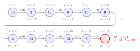
Figure 86: Searching for the inverse of \([10]\) in \(\mathbb{Z}_{17}\). Starting at 10, each hop adds 10 and reduces mod 17; the grey number under a class is the unreduced total, shown where 17 had to be taken off. Because 17 is prime, the hops pass through non-zero classes only and cannot repeat before every non-zero class has appeared, so the class 1 is certain to turn up. It turns up at the twelfth multiple, so \(10 \cdot 12 \equiv 1 \pmod{17}\) and \([10]^{-1} = [12]\).
Reducing the answer. \(-36 = (-2) \cdot 17 - 2\), so \([-36] = [-2]\), and \([-2] = [-2 + 17] = [15]\). A shorter path is to notice \([12] = [-5]\), so \(x = [-5] \cdot [-3] = [15]\) straight away.
Check: \(10(15) + 9 = 159 = 10 \cdot 17 - 11 \equiv -11 \equiv 6 \pmod{17}\). \(\checkmark\)
The integers \(y\) with \(10y + 9 \equiv 6 \pmod{17}\) are the members of \([15] = \{\dots, -19, -2, 15, 32, \dots\}\). The smallest positive one is \(\mathbf{y = -2 + 17 = 15}\). The representative \(-2\) is a correct name for the class, but it is not the positive integer the question asks for.
See also
- [fields] — the definition, examples and non-examples, why \(\mathbb{Z}_n\) is a field exactly when \(n\) is prime, and solving equations
- subgroups-and-cyclic-groups — subgroups, \(\langle a \rangle\), and cyclic groups
- integers-modulo-n — \(\mathbb{Z}_n\), and multiplicative inverses mod \(p\)
- [groups] — the four group properties used in conditions (1) and (2)
- cayley-tables — reading closure and inverses off a table, as in the \(\mathbb{Z}_4\) question
- 2026-10-06-elementary-properties-of-groups — Lecture 27 · 2026-10-12-introduction-to-counting — Lecture 29
- practice-problems — §34, where Q4 shows that \((\mathbb{Z}_{11} - \{[0]\}, \cdot)\) is cyclic
- practice-problems — §36, with full worked solutions
Week 11
Lecture 29 — Introduction to Counting
Counting the outcomes of a process without listing them. The multiplication rule handles a choice made in steps, the addition rule handles a count that splits into separate cases, and subtracting from the total handles “at least one”. Together they count permutations, first of a whole set and then with conditions on the first few positions. Pre-work: Video 037 (Introduction to Counting). The rules, why they work and where they go wrong are collected in counting-principles, and choosing elements without regard to order carries on in 2026-10-13-counting-selections.
Goals
- Learn how to solve simple counting problems.
- Learn how to count permutations when restrictions are added.
- Learn some counting techniques and understand why they work.
Two questions to keep in mind:
- How do you count arrangements of only some of the elements, the \(r\)-permutations? A four-symbol number plate with no repeated symbol is one, in the number plates, part (b). The general count is in counting-principles.
- When do you add and when do you multiply? Multiply across the steps of one choice, add across cases that cannot both happen. The summary at the end.
Worked: arranging \(1, 2, 3, 4, 5\)
How many permutations of \(\{1, 2, 3, 4, 5\}\) are there? Explain your reasoning.
Build the arrangement one position at a time. Any of the 5 numbers can go first. Whichever it was, 4 numbers are left for the second position, then 3 for the third and 2 for the fourth, and the last position takes the one number remaining. So there are
\[5 \times 4 \times 3 \times 2 \times 1 = 5! = 120\]
permutations.
Following one arrangement through shows what “4 left” means. Put 3 first. The second position can then take 1, 2, 4 or 5, which is 4 options. Put 4 there, and the third can take 1, 2 or 5. Put 2, and the fourth can take 1 or 5. Put 1, and the last must be 5. That builds \(3\,4\,2\,1\,5\). Starting with 1 instead of 3 leaves a different four for the second position, \(\{2, 3, 4, 5\}\), but still four of them. What the multiplication rule needs is that the number of options at each step is the same whatever was chosen before, even though the options themselves change. As a possibility tree, the start has 5 branches, each of those has 4, each of those 3, and so on, so there are \(5 \times 4 \times 3 \times 2 \times 1\) leaves, one per permutation.
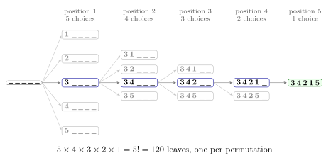
Figure 87: Part of the possibility tree for arranging \({1, 2, 3, 4, 5}\), one position at a time. Only the path that builds \(3,4,2,1,5\) is followed; every grey node branches in the same way. At each level every node has the same number of branches, 5, then 4, 3, 2 and 1, whichever numbers have been used, so the tree has \(5 \times 4 \times 3 \times 2 \times 1 = 120\) leaves, one for each permutation.
The complete tree for three elements, small enough to draw in full, is in counting-principles.
Worked: one odd and one even
How many ways are there to choose two of the numbers \(1, 2, 3, 4, 5, 6, 7, 8, 9\) if one of the chosen numbers is odd and the other is even?
Sort the nine numbers by parity:
\[D = \{1, 3, 5, 7, 9\}, \qquad E = \{2, 4, 6, 8\}.\]
There are five odd numbers to choose from and four even ones. Every odd number goes with every even number, so the valid choices fill a grid with one row per odd number and one column per even number:
| \(2\) | \(4\) | \(6\) | \(8\) | |
|---|---|---|---|---|
| \(\mathbf{1}\) | 1 and 2 | 1 and 4 | 1 and 6 | 1 and 8 |
| \(\mathbf{3}\) | 3 and 2 | 3 and 4 | 3 and 6 | 3 and 8 |
| \(\mathbf{5}\) | 5 and 2 | 5 and 4 | 5 and 6 | 5 and 8 |
| \(\mathbf{7}\) | 7 and 2 | 7 and 4 | 7 and 6 | 7 and 8 |
| \(\mathbf{9}\) | 9 and 2 | 9 and 4 | 9 and 6 | 9 and 8 |
For each of the 5 choices of odd number there are 4 choices of even number, so there are \(5 \times 4 = 20\) ways. In set terms the grid is the Cartesian product \(D \times E\), the ordered pairs \((a, b)\) with \(a\) odd and \(b\) even, and
\[|D \times E| = |D| \times |E| = 5 \times 4 = 20\]
The order of choosing does not matter. Choosing 1 and 2 is the same as choosing 2 and 1. Even so, the ordered pairs count the unordered choices exactly: every valid choice has exactly one odd member, so writing the odd one first turns each choice into exactly one pair \((a, b) \in D \times E\), and each pair comes from exactly one choice. That matching is a bijection, and matched finite sets have the same size (cardinality). Each choice appears once in the grid, in the row of its odd number. Counting “first number picked, then second” instead gives \(5 \times 4 + 4 \times 5 = 40\), which counts every pair twice.
Choosing from \(\{1, \dots, 8\}\): prime, composite or neither
Let \(X = \{1, 2, 3, 4, 5, 6, 7, 8\}\), so \(|X| = 8\). Every element of \(X\) is in exactly one of
\[P = \{2, 3, 5, 7\}\ \text{(prime)}, \qquad C = \{4, 6, 8\}\ \text{(composite)}, \qquad \{1\}\ \text{(neither)}.\]
1 is neither prime nor composite, and both questions turn on it.
Worked: one prime and one composite
How many ways are there to choose two numbers from \(X\) such that one is prime and the other is composite?
A. 7 \(\quad\) B. 12 \(\quad\) C. 15 \(\quad\) D. 24
B, 12. As with odd and even, a valid choice has exactly one prime member and one composite member, so it matches exactly one ordered pair in \(P \times C\):
\[|P \times C| = |P| \times |C| = 4 \times 3 = 12.\]
The other options each make a recognisable mistake. 24 counts every pair twice, once in each order. 7 is \(4 + 3\), adding where both choices are made and so the counts multiply. 15 is \(5 \times 3\), which treats 1 as a prime.
Worked: prime or composite
How many ways are there to choose one number from \(X\) such that it is prime or composite?
A. 3 \(\quad\) B. 7 \(\quad\) C. 8 \(\quad\) D. 12
B, 7. Every element of \(X\) except 1 is prime or composite, so the count is
\[|X - \{1\}| = 8 - 1 = 7.\]
That counts by the complement: take everything and remove what is excluded. Counting the wanted numbers directly gives the same. No number is both prime and composite, so \(P\) and \(C\) are disjoint, and by the addition rule \(|P \cup C| = |P| + |C| = 4 + 3 = 7\). Only one number is chosen, and it is a prime or a composite, so the counts add. 12 multiplies as if two numbers were chosen, 8 forgets to leave out 1, and 3 counts only the composites.
The two counts use the same sets and the same sizes, 4 and 3, and differ only in how many numbers are chosen. One number from either of two disjoint sets adds their sizes. One number from each of them multiplies.
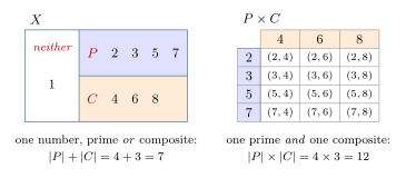
Figure 88: \(X = {1, \dots, 8}\) split into the primes \(P\), the composites \(C\), and 1, which is neither. Left: one number that is prime or composite is a single choice from the shaded part of \(X\). No number is in both \(P\) and \(C\), so the shaded part has \(4 + 3 = 7\) elements. Right: one prime and one composite is a choice from each part. Every prime can go with every composite, so the choices fill a grid with a row for each prime and a column for each composite, \(4 \times 3 = 12\) cells, the pairs of \(P \times C\). A choice from either part adds the sizes; a choice from each part multiplies them. 1 is in neither count.
Permutations
A permutation of a set of objects is an arrangement of the objects into an order.
How many permutations of \(\{1, 2, 3, 4\}\) are there? For each of the four choices for the first number, there are three ways to choose the second. Once the first two are chosen there are two ways to choose the third, and then the fourth is forced. So there are \(4 \times 3 \times 2 \times 1 = 24\) permutations. Listed in dictionary order they fall into blocks, and the sizes of the blocks are the factors of the product.
Figure 89: The 24 permutations of \({1, 2, 3, 4}\) in dictionary order, as nested blocks. The first number picks the column, 4 ways. Inside a column the second number picks one of 3 boxes, since one number is already used. Inside a box the third number picks one of 2 rows, and the fourth number is whatever is left. Each level splits every block into the same number of pieces, so the total is \(4 \times 3 \times 2 \times 1 = 4! = 24\).
The same reasoning works for any number of objects.
The number of permutations of a set of \(n\) distinct objects is \[n \times (n-1) \times (n-2) \times \cdots \times 2 \times 1 = n!\]
\(n!\) is read “\(n\) factorial”, or “\(n\) bang”. As a product, \(n! = \prod_{i=1}^{n} i\) for \(n \in \mathbb{Z}^{+}\), and \(0! = 1\) by definition (recursive-definitions). The values grow very fast:
| \(n\) | 1 | 2 | 3 | 4 | 5 | 6 | 7 |
|---|---|---|---|---|---|---|---|
| \(n!\) | 1 | 2 | 6 | 24 | 120 | 720 | 5040 |
A bijection from \(\{1, \dots, n\}\) to itself is fixed by listing \(f(1), f(2), \dots, f(n)\), which is a permutation of \(\{1, \dots, n\}\). So the symmetric group \(S_n\) has \(n!\) elements, and \(S_3\) has the six of symmetric-group.
Worked: starting with an even number
How many permutations of the numbers 1, 2, 3, 4, 5 start with an even number?
Fill the restricted position first. The first number must be 2 or 4, so there are 2 choices. Whichever it is, the other four numbers fill the remaining four positions in any order, in \(4! = 24\) ways. So the answer is
\[2 \times 4! = 2 \times 24 = 48.\]
Position by position that is \(2 \times 4 \times 3 \times 2 \times 1\). If 2 goes first, the second position can take any of 1, 3, 4, 5, and 4 is still among them: the even number not chosen is free to go anywhere else.
A check: each of the five numbers starts the same number of permutations, \(4!\) each, and two of the five are even, so the answer is \(\frac{2}{5}\) of the \(5! = 120\) permutations, which is 48.
Worked: starting with a prime
How many permutations of \(\{1, 2, 3, 4, 5, 6, 7\}\) start with a prime number?
A. \(4 \times 6 = 24\) \(\quad\) B. \(4! \times 3! = 144\) \(\quad\) C. \(4 \times 6! = 2880\) \(\quad\) D. \(5 \times 6! = 3600\)
C, 2880. Let \(N = \{1, 2, 3, 4, 5, 6, 7\}\) and \(P = \{2, 3, 5, 7\}\). The first position has \(|P| = 4\) choices. Once it is filled, any of the \(|N| - 1 = 6\) remaining numbers can go second, any of the \(|N| - 2 = 5\) still remaining can go third, and so on down to 1 for the last position:
\[|P| \times (|N| - 1)! = 4 \times 6! = 4 \times 720 = 2880.\]
If 5 goes first, for instance, the other six positions are filled from \(\{1, 2, 3, 4, 6, 7\}\). That includes the primes 2, 3 and 7. Only the first position is restricted, and the rest is an unrestricted arrangement of what is left.
Figure 90: Counting the permutations of \({1, \dots, 7}\) that start with a prime, one position at a time. The restricted position is filled first, from the 4 primes. Each later position has one fewer number available than the one before, whatever was placed earlier, so the last six positions are an arrangement of the six numbers left: \(6!\) ways. The multiplication rule gives \(4 \times 6! = 2880\).
Each wrong option is a different mistake:
- A, \(4 \times 6\), fills the first two positions and forgets the other five.
- B, \(4! \times 3!\), arranges the four primes among themselves and the three non-primes among themselves. That counts the permutations with all four primes at the front, a much stronger condition.
- D, \(5 \times 6!\), counts 1 as a prime.
Worked: what comes second
- How many permutations of \(\{1, 2, 3, 4, 5, 6, 7\}\) start with a prime number followed by a composite number?
- How many permutations of \(\{1, 2, 3, 4, 5, 6, 7\}\) start with a prime number followed by an odd number?
The sets involved, inside \(N = \{1, 2, 3, 4, 5, 6, 7\}\):
\[P = \{2, 3, 5, 7\}, \qquad C = \{4, 6\}, \qquad D = \{1, 3, 5, 7\}\ \text{(odd)}.\]
(a) Position 1 is a prime, 4 choices. Position 2 is a composite, 2 choices, however position 1 was filled: no prime is composite, so the first choice never uses up a composite. Positions 3 to 7 hold the 5 numbers left, in any order. So
\[|P| \times |C| \times (|N| - 2)! = 4 \times 2 \times 5! = 8 \times 120 = 960.\]
(b) The same approach stalls at position 2. How many odd numbers are left depends on which prime went first. If it was 2, all four odd numbers are still available. If it was 3, 5 or 7, an odd number has been used and only three remain. The multiplication rule needs the count at each step to be the same whatever came before, so split into cases on the first number, and within each case it is the same every time.
- Case 1: the first number is even, so it is 2. One choice for position 1, then \(|D| = 4\) for position 2, then \(5!\) for the rest: \(1 \times 4 \times 5!\).
- Case 2: the first number is odd, so it is 3, 5 or 7. That is \(|P| - 1 = 3\) choices for position 1, then \(|D| - 1 = 3\) for position 2, since the first number used up an odd number, then \(5!\) for the rest: \(3 \times 3 \times 5!\).
Every qualifying permutation is in exactly one case, because its first number either is 2 or is not. So the addition rule adds them:
\[1 \times 4 \times 5! + 3 \times 3 \times 5! = (4 + 9) \times 5! = 13 \times 120 = 1560.\]
Multiplying straight through, \(4 \times 4 \times 5! = 1920\), is wrong: it allows four odd numbers in position 2 after an odd prime, when only three are left.
Figure 91: The possibility tree for the first two positions of a permutation of \({1, \dots, 7}\) that starts with a prime followed by an odd number. The tree is lopsided: after 2 there are four odd numbers to follow, but after 3, 5 or 7 there are only three, because the first number used one of them up. So the multiplication rule cannot be applied in one go. Splitting on the first number gives two cases that are each regular, \(1 \times 4\) and \(3 \times 3\) starts. They add to 13, and each start is completed by arranging the other five numbers.
Worked: permutations of \(\{1, \dots, 60\}\)
- How many permutations of \(\{1, 2, \dots, 60\}\) start with an even number followed by a number that is divisible by 3?
- How many permutations of \(\{1, 2, \dots, 60\}\) have at least one even number in the first two positions?
Let \(N = \{1, 2, \dots, 60\}\), so \(|N| = 60\), and
\[E = \{n \in N : n \text{ is even}\}, \qquad T = \{n \in N : 3 \mid n\}.\]
Then \(|E| = 30\) and \(|T| = 20\). The numbers in both are the multiples of 6, so \(|E \cap T| = 10\), and \(|E - T| = 30 - 10 = 20\).
(a) This is the difficulty of prime followed by odd again. An even first number that is also a multiple of 3 uses up one of the multiples of 3, and one that is not leaves all 20 of them. So split on whether the first number is divisible by 3.
- Case 1: the first number is divisible by 3. It is in \(E \cap T\), 10 choices. Position 2 takes any of the other \(|T| - 1 = 19\) multiples of 3. The remaining 58 numbers go in any order: \(10 \times 19 \times 58!\).
- Case 2: the first number is not divisible by 3. It is in \(E - T\), 20 choices. Position 2 takes any of the \(|T| = 20\) multiples of 3. Then \(58!\) for the rest: \(20 \times 20 \times 58!\).
\[\text{total} = 10 \times 19 \times 58! + 20 \times 20 \times 58! = (190 + 400) \times 58! = 590 \times 58!.\]
That is about \(1.39 \times 10^{81}\), and the factorial form is the sensible way to leave it.
Figure 92: The even numbers \(E\) and the multiples of 3, \(T\), in \({1, \dots, 60}\), with the size of each region. The two cases of part (a) are the two parts of \(E\). If the first number comes from the overlap, the multiples of 6, it is itself a multiple of 3 and leaves only 19 for the second position. If it comes from the rest of \(E\), all 20 multiples of 3 are still available.
(b) “At least one even number in the first two positions” happens in three ways, writing E for even and O for odd: EE, EO and OE. Each is a regular count.
- EE: 30 even numbers for position 1, then 29 for position 2: \(30 \times 29 \times 58!\).
- EO: 30 even, then 30 odd: \(30 \times 30 \times 58!\).
- OE: 30 odd, then 30 even: \(30 \times 30 \times 58!\).
\[(30 \times 29 + 30 \times 30 + 30 \times 30) \times 58! = (870 + 900 + 900) \times 58! = 2670 \times 58!.\]
Or count the complement. The only way to fail is OO, both odd. So
\[\#\text{permutations} = (\text{all permutations, no restriction}) - (\text{permutations starting odd, odd}) = 60! - 30 \times 29 \times 58!.\]
The two answers agree: \(60! = 60 \times 59 \times 58! = 3540 \times 58!\), and \(3540 - 870 = 2670\). The complement is one case to count instead of three, which is why it is the natural tool for “at least one”.
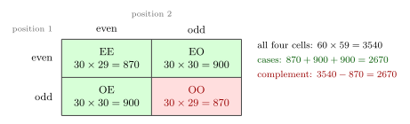
Figure 93: Every permutation of \({1, \dots, 60}\) falls in exactly one cell, according to the parity of its first two numbers; each count shown is then multiplied by \(58!\) for the other positions. A diagonal cell is \(30 \times 29\) because the second number has the same parity as the first and one of them is used up. The three shaded green cells are the permutations with at least one even number in the first two positions. They can be added cell by cell, or found as everything, \(60 \times 59 = 3540\), minus the one red cell where both are odd. Both give \(2670 \times 58!\).
Worked: number plates
In a certain state, number plates consist of four, five or six symbols chosen from the 26 letters of the alphabet together with the ten digits \(0, 1, \dots, 9\).
(a) How many distinct number plates are possible if repetition of symbols is allowed?
(b) How many distinct number plates are possible if repetition of symbols is not allowed?
(c) How many distinct number plates contain at least one repeated symbol?
(d) How many distinct number plates contain exactly one digit?
The symbols form a set \(S\) of \(|S| = 26 + 10 = 36\), adding because no symbol is both a letter and a digit. A plate is ordered: \(\mathtt{AB12}\) and \(\mathtt{21BA}\) are different plates. So a plate of length \(k\) is a sequence of \(k\) symbols. Every plate has exactly one length, so in each part the plates split into three cases, of length 4, 5 and 6, which add.
(a) Repetition allowed. Each position can be any of the 36 symbols, whatever is in the other positions. A four-symbol plate can be made in \(36 \times 36 \times 36 \times 36 = 36^4\) ways, and in general a \(k\)-symbol plate in \(36^k\) ways.
\[36^4 + 36^5 + 36^6 = 1\,679\,616 + 60\,466\,176 + 2\,176\,782\,336 = 2\,238\,928\,128.\]
(b) Repetition not allowed. Each symbol placed leaves one fewer for the positions after it. A four-symbol plate can be made in
\[36 \times 35 \times 34 \times 33 = \frac{36!}{32!} = \frac{36!}{(36 - 4)!}\]
ways. It is an ordered selection of 4 of the 36 symbols, a 4-permutation of \(S\) (counting-principles).
\[\begin{aligned} &36 \times 35 \times 34 \times 33 \\ +\ &36 \times 35 \times 34 \times 33 \times 32 \\ +\ &36 \times 35 \times 34 \times 33 \times 32 \times 31 \end{aligned} \;=\; 1\,413\,720 + 45\,239\,040 + 1\,402\,410\,240 \;=\; 1\,449\,063\,000.\]
(c) At least one repeated symbol. A plate has at least one repeated symbol exactly when it is not a plate with no repeats. The plates in (b) are among the plates in (a), with the same lengths, so subtract:
\[\text{part (a)} - \text{part (b)} = 2\,238\,928\,128 - 1\,449\,063\,000 = 789\,865\,128.\]
Counted directly, “at least one repeat” would need cases for which symbol repeats, where and how often. The complement avoids all of that.
(d) Exactly one digit. Repetition is allowed here, as in (a): the letters may repeat, and with only one digit the digit cannot. Write \(D = \{0, 1, \dots, 9\}\) and \(L = \{\mathtt{A}, \mathtt{B}, \dots, \mathtt{Z}\}\). For a four-symbol plate with its digit first, the positions hold a digit, a letter, a letter and a letter:
\[|D| \times |L| \times |L| \times |L| = 10 \times 26^3.\]
The digit can be in any of the 4 positions, and those are 4 disjoint cases of the same size, so a four-symbol plate with exactly one digit can be made in \(4 \times 10 \times 26^3\) ways. Equivalently, choose the digit’s position (4 ways), then the digit (10), then the three letters (\(26^3\)). Doing the same for each length and adding,
\[4 \times 10 \times 26^3 + 5 \times 10 \times 26^4 + 6 \times 10 \times 26^5 = 703\,040 + 22\,848\,800 + 712\,882\,560 = 736\,434\,400.\]
If repetition were not allowed, only the letters would change: \(26 \times 25 \times 24\) in place of \(26^3\), and so on.
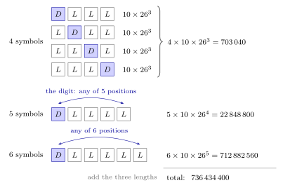
Figure 94: Plates with exactly one digit, \(D\), and letters, \(L\), everywhere else. A four-symbol plate has its digit in one of four positions, and each of those four disjoint cases is filled in \(10 \times 26^3\) ways, so the four rows together give \(4 \times 10 \times 26^3\). Five- and six-symbol plates work the same way, with 5 and 6 positions for the digit. Within a length the rule is multiply; across the three lengths, which no plate can share, it is add.
When to add and when to multiply
Every question above used one or more of three moves.
| Move | When | Examples here |
|---|---|---|
| Multiply | One outcome is built in steps, and the number of options at each step is the same whatever was chosen before. | \(5!\) arrangements; one odd and one even, \(5 \times 4\); prime then composite, \(4 \times 2 \times 5!\) |
| Add | The outcomes split into cases that cannot happen together, and every outcome is in one of them. | prime or composite, \(4 + 3\); prime then odd, \((4 + 9) \times 5!\); plates of length 4, 5 or 6 |
| Subtract | What is not wanted is easier to count than what is. | \(\lvert X - \{1\} \rvert = 8 - 1\); \(60! - 30 \times 29 \times 58!\); plates with a repeat, (a) \(-\) (b) |
“Followed by” and “one from each” are steps, so they multiply. An “or” between alternatives that exclude each other is a case split, so it adds. When a step’s count does depend on an earlier choice, split on that choice: inside each case the count is fixed, so the cases multiply out separately and then add. The rules, with the reasons and the common traps, are in counting-principles.
See also
- counting-principles — the multiplication and addition rules, possibility trees, the complement, permutations and \(r\)-permutations
- counting-selections — the four kinds of selection, ordered or not and with or without repeats; a number plate is an ordered one
- sets-and-set-notation — \(|A \times B| = |A| \times |B|\), the two-step multiplication rule
- recursive-definitions — \(n!\) defined recursively, with \(0! = 1\)
- symmetric-group — the \(n!\) bijections of \(\{1, \dots, n\}\) as a group
- 2026-10-08-definitions-and-examples-of-fields — Lecture 28 · 2026-10-13-counting-selections — Lecture 30
- practice-problems — §37, with full worked solutions
Lecture 30 — Counting Selections
Selecting \(r\) objects from \(n\): the four cases that come from asking whether order matters and whether repeats are allowed, a formula for each, and counting problems where the selection is restricted. Pre-work: Video 038 (Counting Selections). The four cases and their formulas, the ways of handling restrictions, counting “at least” through the complement, and arrangements of words with repeated letters are all collected in counting-selections. The multiplication, addition and difference rules and the permutations they rest on are in counting-principles. The note starts by finishing the number-plate question from 2026-10-12-introduction-to-counting.
Goals
- Understand the different cases for selections of \(r\) objects from \(n\).
- Learn how to count selections in each case, and when restrictions are added.
- Gain confidence with solving counting problems.
Three questions to keep in mind:
- How is \(n\) choose \(r\) calculated? The formulas, and why it divides by \(r!\).
- How many distinct arrangements do the letters of BANANAS have? After BARBARA, which is the same kind of problem.
- How many ways are there to choose 7 candies from 4 colours? The fourth case, which counts them as strings of X’s and bars.
Finishing the number plates
In a certain state, number plates consist of four, five or six symbols chosen from the 26 letters of the alphabet together with the ten digits \(0, 1, \dots, 9\).
(a) How many distinct number plates are possible if repetition of symbols is allowed?
(b) How many distinct number plates are possible if repetition of symbols is not allowed?
(c) How many distinct number plates contain at least one repeated symbol?
(d) How many distinct number plates contain exactly one digit?
The full working is in 2026-10-12-introduction-to-counting. In short: there are \(26 + 10 = 36\) symbols, a plate is an ordered selection of them, and each part is counted separately for 4, 5 and 6 symbols and then added.
| Count | Answer | |
|---|---|---|
| (a) repeats allowed | \(36^4 + 36^5 + 36^6\) | \(2\,238\,928\,128\) |
| (b) no repeats | \(36 \cdot 35 \cdot 34 \cdot 33 \;+\; 36 \cdot 35 \cdots 32 \;+\; 36 \cdot 35 \cdots 31\) | \(1\,449\,063\,000\) |
| (c) at least one repeat | (a) \(-\) (b) | \(789\,865\,128\) |
| (d) exactly one digit | \(4 \cdot 10 \cdot 26^3 + 5 \cdot 10 \cdot 26^4 + 6 \cdot 10 \cdot 26^5\) | \(736\,434\,400\) |
For (d), a \(k\)-symbol plate has \(k\) places the digit can go, 10 choices of digit, and 26 letters for each of the other \(k - 1\) places. For four symbols with the digit first that is \(10 \cdot 26 \cdot 26 \cdot 26 = 10 \cdot 26^3\), and the digit can be in any of the 4 places, so \(4 \cdot 10 \cdot 26^3 = 703\,040\). The five- and six-symbol plates add \(22\,848\,800\) and \(712\,882\,560\).
Two ideas from this question run through the rest of the note. The four-symbol term of (b) is
\[36 \cdot 35 \cdot 34 \cdot 33 = \frac{36!}{32!} = \frac{36!}{(36-4)!},\]
the first of the four formulas. And (c) counts “at least one” as everything minus “none”, which is how the vowel, the digit 5 and two evens questions are done.
Four ways to select
Selecting 2 numbers from \(\{1, 2, 3, 4\}\) gives four different answers, depending on two questions. Does the order matter, so that 12 and 21 are different selections? Can a number be chosen twice, as in 11? Write each selection as the two numbers in the order chosen.
| The selections | Count | |
|---|---|---|
| (1) ordered, without repeats | 12, 13, 14, 21, 23, 24, 31, 32, 34, 41, 42, 43 | 12 |
| (2) ordered, with repeats | the twelve above, and 11, 22, 33, 44 | 16 |
| (3) unordered, without repeats | 12, 13, 14, 23, 24, 34 | 6 |
| (4) unordered, with repeats | 11, 12, 13, 14, 22, 23, 24, 33, 34, 44 | 10 |
In the unordered cases each selection is written with its smaller number first, since 21 is the same selection as 12.
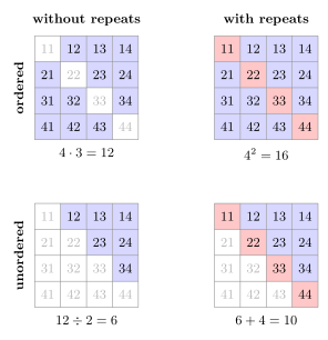
Figure 95: Every way of picking a first and a second number from \({1, 2, 3, 4}\) is a cell of a 4 by 4 grid, first number down the side and second along the top. Each case of selection keeps a different part of the grid. Ordered with repeats keeps all 16. Ordered without repeats drops the diagonal, the repeats 11, 22, 33, 44, leaving 12. Unordered selections keep one cell of each mirror pair, since 21 is the same selection as 12. Without repeats that is the 6 cells above the diagonal, half of the 12. With repeats the diagonal comes back, and there are \(6 + 4 = 10\).
Which case is which
Four questions, one for each case:
- How many different possibilities are there for first, second and third in a race of 10 people? Ordered, since first and second are different prizes, and without repeats, since nobody finishes twice. Case (1).
- How many 3-digit passwords are there? Ordered, since 123 and 321 are different passwords, and with repeats, since 112 is allowed. Case (2).
- How many 3-element subsets of \(\{1, 2, 3, 4, 5, 6, 7, 8, 9, 10\}\) are there? A set has no order and no repeated elements. Case (3).
- How many ways are there to select 3 chocolate bars when there are 10 different kinds to choose from? The bars end up in one pile, so there is no order, but two bars of the same kind are allowed. Case (4).
All four select \(r = 3\) from \(n = 10\). Their answers, 720, 1000, 120 and 220, come from the formulas below.
The formulas
With \(n = 10\) and \(r = 3\) in the right-hand column:
| Case | Formula | Selecting 3 from 10 |
|---|---|---|
| (1) ordered, without repeats | \(\dfrac{n!}{(n-r)!} = \underbrace{n(n-1)\cdots(n-r+1)}_{r \text{ factors}}\) | \(10 \cdot 9 \cdot 8 = 720\) |
| (2) ordered, with repeats | \(n^r = \underbrace{n \cdot n \cdots n}_{r \text{ factors}}\) | \(10^3 = 10 \cdot 10 \cdot 10 = 1000\) |
| (3) unordered, without repeats | \(\dbinom{n}{r} = \dfrac{n!}{r!\,(n-r)!} = \dfrac{n(n-1)\cdots(n-r+1)}{r(r-1)\cdots 1}\) | \(\dfrac{10 \cdot 9 \cdot 8}{3 \cdot 2 \cdot 1} = 120\) |
| (4) unordered, with repeats | \(\dbinom{n+r-1}{r} = \dfrac{n(n+1)\cdots(n+r-1)}{r(r-1)\cdots 1}\) | \(\dfrac{10 \cdot 11 \cdot 12}{3 \cdot 2 \cdot 1} = 220\) |
Case (1) is the multiplication rule with one fewer option at each step. Case (2) is the multiplication rule with all \(n\) options every time. Each formula is explained in counting-selections.
Case (4) is extension material. It is not assessable in MATH1061. It is Section 9.6 of Epp, and it is covered in MATH2302.
Calculating \(n\) choose \(r\). \(\binom{n}{r}\) is read “\(n\) choose \(r\)” and also written \(C(n, r)\). It is the number of \(r\)-element subsets of an \(n\)-element set. To work it out, write \(r\) factors counting down from \(n\) over \(r\) factors counting down from \(r\), and cancel:
\[\binom{10}{3} = \frac{10!}{3!\,7!} = \frac{10 \cdot 9 \cdot 8}{3 \cdot 2 \cdot 1} = \frac{720}{6} = 120.\]
The \(7!\) in \(10!\) cancels against the \(7!\) underneath, which is why only three factors are left on top. Case (4) is the same except that the top counts up from \(n\).
Worked: choosing candies
How many ways are there to choose 7 candies when there are 4 colours, red, blue, yellow and pink, any colour can be taken any number of times, and candies of the same colour are identical?
The candies are not ordered and colours can repeat, so this is case (4), with \(n = 4\) colours and \(r = 7\) candies.
A selection is settled by how many of each colour are taken. Write an X for each candy, the red ones first, then blue, yellow and pink, and put a bar \(|\) between one colour and the next. Two red, one blue, four yellow and no pink is
\[\mathrm{XX}\,|\,\mathrm{X}\,|\,\mathrm{XXXX}\,|\]
and two red, two blue, one yellow and two pink is
\[\mathrm{XX}\,|\,\mathrm{XX}\,|\,\mathrm{X}\,|\,\mathrm{XX}.\]
Each selection corresponds to an arrangement of 7 X’s and 3 bars, and each such arrangement is one selection. An arrangement is fixed by choosing which 3 of the 10 positions hold the bars, so there are
\[\binom{10}{3} = \frac{10!}{3!\,7!} = \frac{10 \cdot 9 \cdot 8}{3 \cdot 2 \cdot 1} = 120\]
selections. The formula agrees: \(\binom{n+r-1}{r} = \binom{4+7-1}{7} = \binom{10}{7} = \binom{10}{3} = 120\). The two selections are drawn in counting-selections.
Ordered and unordered: dividing by \(r!\)
Cases (1) and (3) are linked. Take the selections of 3 objects from \(\{1, 2, 3, 4\}\) without repeats.
Ordered, there are \(4 \cdot 3 \cdot 2 = 24\):
| 123 | 124 | 134 | 234 |
| 132 | 142 | 143 | 243 |
| 213 | 214 | 314 | 324 |
| 231 | 241 | 341 | 342 |
| 312 | 412 | 413 | 423 |
| 321 | 421 | 431 | 432 |
Unordered, there are 4: 123, 124, 134, 234.
Each column of the table holds the same three numbers in all \(3 \cdot 2 \cdot 1 = 3! = 6\) possible orders, and forgetting the order collapses the whole column to one subset. So
\[\binom43 = \frac{24}{3!} = \frac{4 \cdot 3 \cdot 2}{3 \cdot 2 \cdot 1} = 4.\]
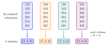
Figure 96: The 24 ordered selections of 3 objects from \({1, 2, 3, 4}\), sorted by which three numbers they use. Each column holds one set of three numbers in all \(3! = 6\) of its orders. Ignoring order merges each column into a single subset, so there are \(24 \div 3! = 4\) subsets. In general each \(r\)-element subset accounts for \(r!\) of the ordered selections, which is why \(\binom{n}{r}\) is the ordered count divided by \(r!\).
The same thing happens for any \(n\) and \(r\). Every \(r\)-element subset turns up \(r!\) times among the ordered selections, once in each order, so
\[\binom{n}{r} = \frac{1}{r!} \cdot \frac{n!}{(n-r)!} = \frac{n!}{r!\,(n-r)!}.\]
Worked: 8-letter passwords
A certain website requires users to choose a password consisting of 8 lower-case letters of the 26-letter alphabet \(a, b, c, d, \dots, x, y, z\). How many different passwords are there?
A. \(26!\)
B. \(8!\)
C. \(26 \times 25 \times 24 \times 23 \times 22 \times 21 \times 20 \times 19\)
D. \(8^{26}\)
E. \(26^8\)
Answer: E, \(26^8 = 208\,827\,064\,576\).
A password is ordered: cat and cta are different passwords. And it allows repeats: nothing stops a letter being used twice. So it is case (2) with \(n = 26\) letters and \(r = 8\) positions, and each of the 8 positions has 26 choices.
The other options:
- A, \(26!\), counts the ways to put all 26 letters in a row, each used once.
- B, \(8!\), counts the orders of 8 letters already chosen.
- C, \(26 \cdot 25 \cdots 19\), counts 8-letter passwords with no letter repeated, which is case (1).
- D, \(8^{26}\), has \(n\) and \(r\) the wrong way round. It would count 26 positions with 8 choices each.
Worked: passwords with a vowel
How many of the passwords from the question above contain a vowel? (There are 5 vowels: \(a, e, i, o, u\).)
“Contain a vowel” means at least one vowel. It could be 1, 2, 3, up to 8 vowels. Counting those cases one by one is long. Their opposite, no vowel at all, is one product: each of the 8 positions is one of the \(26 - 5 = 21\) consonants.
\[\#(\text{passwords with no vowel}) = 21^8.\]
Every password either contains a vowel or does not, so
\[\begin{aligned} \#(\text{passwords with at least one vowel}) &= \#(\text{all passwords}) - \#(\text{passwords with no vowel}) \\ &= 26^8 - 21^8 \\ &= 208\,827\,064\,576 - 37\,822\,859\,361 \\ &= 171\,004\,205\,215. \end{aligned}\]
Worked: integers containing a 5
How many of the integers from 0 to 9999 contain the digit 5?
Make every number four digits long by writing leading zeros: 0 is 0000, 1 is 0001, 42 is 0042. The added zeros never contain a 5, so this does not change which numbers contain a 5. Now the integers from 0 to 9999 are exactly the strings of 4 digits, and each of the 4 positions has 10 choices:
\[\#(\text{integers from 0 to 9999}) = 10 \cdot 10 \cdot 10 \cdot 10 = 10^4.\]
A number with no 5 has 9 choices in each position, \(\{0, 1, 2, 3, 4, 6, 7, 8, 9\}\):
\[\#(\text{those with no 5}) = 9^4 = 6561.\]
So
\[\#(\text{those containing at least one 5}) = 10^4 - 9^4 = 10\,000 - 6561 = 3439.\]
The long way, as a check. Count by the exact number of 5s and add. For exactly \(k\) fives, choose which \(k\) of the 4 positions hold them, \(\binom4k\) ways, and fill each of the others with one of the 9 other digits:
\[\begin{aligned} &\#(\text{one 5}) + \#(\text{two 5s}) + \#(\text{three 5s}) + \#(\text{four 5s}) \\ &\quad= \binom41 9^3 + \binom42 9^2 + \binom43 9 + \binom44 \\ &\quad= 2916 + 486 + 36 + 1 = 3439. \end{aligned}\]
Same answer, four terms instead of two.
Worked: 5 immediately followed by 6
- How many ordered selections without repetition of 4 elements are there from the set \(\{1, 2, \dots, 10\}\)?
- How many ordered selections without repetition of 4 elements from the set \(\{1, 2, \dots, 10\}\) have 5 immediately followed by 6?
(a) Case (1) with \(n = 10\) and \(r = 4\):
\[\frac{n!}{(n-r)!} = \frac{10!}{(10-4)!} = 10 \cdot 9 \cdot 8 \cdot 7 = 5040.\]
Four positions, with 10, 9, 8 and 7 numbers left for them in turn.
(b) Place the restricted part first. “5 immediately followed by 6” is a block of two neighbouring positions, 5 then 6. In 4 positions the block can start at position 1, 2 or 3. It cannot start at position 4, because the 6 would have nowhere to go. Wherever the block is, the two positions it leaves are filled, in order, from the 8 numbers other than 5 and 6: 8 choices for the first and 7 for the second.
\[\#(\text{choices}) = 3\,(1 \cdot 1 \cdot 8 \cdot 7) = 3 \cdot 8 \cdot 7 = 21 \cdot 8 = 168.\]
The 1s are the positions of 5 and 6, which have no choice once the block is placed.
Figure 97: The ordered selections of 4 from \({1, \dots, 10}\) with 5 immediately followed by 6, counted one position at a time. Each box holds the number of choices for its position. The block 5 then 6, shaded, takes two neighbouring positions, and once it is placed those positions have 1 choice each; the value forced into each is written above it. The block fits in three places. Wherever it goes, the two positions left over take two of the other 8 numbers in order, 8 choices and then 7. A fourth placement would put the 5 last, leaving no room for the 6. So there are \(3,(1 \cdot 1 \cdot 8 \cdot 7) = 168\) selections.
Worked: 3-element subsets of a 6-element set
How many 3-element subsets of \(\{1, 2, 3, 4, 5, 6\}\) are there?
A. 18
B. 20
C. 60
D. 120
Answer: B, 20.
A subset is unordered and has no repeated elements, so this is case (3):
\[\binom63 = \frac{6!}{3!\,3!} = \frac{6 \cdot 5 \cdot 4}{3 \cdot 2 \cdot 1} = 20.\]
The other options:
- D, 120, is \(6 \cdot 5 \cdot 4\), the number of ordered selections. Each subset is counted \(3! = 6\) times in it.
- C, 60, is \(120 \div 2\). It divides by 2 where it should divide by \(3! = 6\).
- A, 18, is \(6 \cdot 3\), which doesn’t count any kind of selection.
Worked: three even and two odd
How many 5-element subsets of \(\{1, 2, \dots, 11\}\) contain 3 even numbers and 2 odd numbers?
Split the set into its evens and its odds:
\[E = \{2, 4, 6, 8, 10\},\ |E| = 5, \qquad O = \{1, 3, 5, 7, 9, 11\},\ |O| = 6.\]
A subset of the required kind is a choice of 3 elements of \(E\) together with a choice of 2 elements of \(O\). The two choices are independent, and every pair of them gives a different subset, so by the multiplication rule
\[\begin{aligned} \#(\text{subsets}) &= \#(\text{ways to choose 3 evens}) \cdot \#(\text{ways to choose 2 odds}) \\ &= \binom53 \binom62 = \frac{5!}{3!\,2!} \cdot \frac{6!}{2!\,4!} = \frac{5 \cdot 4}{2} \cdot \frac{6 \cdot 5}{2} = 10 \cdot 15 = 150. \end{aligned}\]
Figure 98: The 5-element subsets of \({1, \dots, 11}\) with 3 even and 2 odd numbers. The set splits into its evens \(E\) and its odds \(O\), and a subset of this kind is 3 elements taken from \(E\) together with 2 taken from \(O\). One of them, \({2, 3, 6, 7, 10}\), is shaded. The two choices are made separately, and whichever 3 evens are taken, any 2 odds can go with them, so the numbers of ways multiply: \(\binom53 \binom62 = 10 \cdot 15 = 150\).
Worked: at least two even numbers
How many 7-element subsets of \(\{1, 2, \dots, 21\}\) contain at least two even numbers?
Let \(N = \{1, 2, \dots, 21\}\), so \(|N| = 21\). Its evens are \(E = \{2, 4, \dots, 20\}\) with \(|E| = 10\), and its odds are \(O = \{1, 3, \dots, 21\}\) with \(|O| = 11\).
“At least two” could be 2, 3, 4, 5, 6 or 7 evens. Its opposite is “no evens” or “exactly one even”, two cases instead of six. So
\[\#(\text{at least 2 evens}) = \#(\text{all}) - \#(\text{no evens}) - \#(\text{exactly 1 even}).\]
- All. Any 7 of the 21 numbers: \(\binom{21}{7} = 116\,280\).
- No evens. All 7 come from the 11 odds: \(\binom{11}{7} = \binom{11}{4} = 330\).
- Exactly one even. Choose the one even from 10 and the other six numbers from the 11 odds: \(\binom{10}{1}\binom{11}{6} = 10 \cdot 462 = 4620\).
Therefore
\[\begin{aligned} \#(\text{subsets with at least 2 evens}) &= \binom{21}{7} - \binom{11}{7} - \binom{11}{6}\binom{10}{1} \\ &= \frac{21!}{14!\,7!} - \frac{11!}{7!\,4!} - \frac{11!}{6!\,5!} \cdot 10 \\ &= 116\,280 - 330 - 4620 \\ &= 111\,330. \end{aligned}\]
The factor of 10 is easy to drop. Without it the answer comes out at \(115\,488\), which is wrong: there are 10 different evens that could be the one even. A direct count over 2 to 7 evens, \(\sum_{k=2}^{7} \binom{10}{k}\binom{11}{7-k}\), gives \(20\,790 + 39\,600 + 34\,650 + 13\,860 + 2310 + 120 = 111\,330\), the same answer.
Figure 99: The 7-element subsets of \({1, \dots, 21}\), split by how many even numbers they contain. Every subset has none, exactly one, or at least two, and no subset is in two of these parts. So the count wanted, shaded, is the total minus the other two parts. Exactly one even is a choice of the even, 10 ways, times a choice of six odds. The widths are not to scale.
Worked: arranging BARBARA
How many distinct arrangements of the letters in the word BARBARA are there?
The letters are B, A and R: two B’s, three A’s and two R’s, 7 letters in all. An arrangement puts one letter in each of 7 positions. It is ordered, since ARBAABR and BARBARA are different words, and it has no repeats, since each position gets exactly one letter. If the 7 letters were all different that would make \(7!\) arrangements. They are not, so count it instead by choosing positions for one kind of letter at a time.
- Place the two B’s: choose 2 of the 7 positions, \(\binom72\) ways. It is a choice, not an ordered selection: once the positions are chosen, the two B’s look identical, so it doesn’t matter which B goes in which of the chosen positions.
- Place the three A’s: choose 3 of the 5 positions left, \(\binom53\) ways.
- Place the two R’s: they go in the 2 positions left, \(\binom22 = \frac{2!}{2!} = 1\) way.
For example, B’s in positions 3 and 6, A’s in 1, 4 and 5, and R’s in 2 and 7 give ARBAABR. By the multiplication rule,
\[\begin{aligned} \#(\text{arrangements}) &= \binom72 \binom53 \binom22 = \frac{7!}{2!\,5!} \cdot \frac{5!}{3!\,2!} \cdot \frac{2!}{2!} \\ &= \frac{7 \cdot 6}{2} \cdot \frac{5 \cdot 4}{2} \cdot 1 = 7 \cdot 6 \cdot 5 = 210. \end{aligned}\]
The \(5!\)s cancel, leaving \(\frac{7!}{2!\,3!\,2!}\): the factorial of the length over the factorial of the number of copies of each letter. The stages are drawn, and the general formula derived, in counting-selections. The same formula comes out a second way, by tagging the copies so that all seven letters differ and dividing out the orders of the copies, in 2026-10-19-probability-binomial-coefficients.
Worked: arranging BANANAS
How many distinct arrangements of the letters in the word BANANAS are there?
BANANAS has 7 letters: one B, three A’s, two N’s and one S. Choosing positions as for BARBARA:
\[\binom71\binom63\binom32\binom11 = 7 \cdot 20 \cdot 3 \cdot 1 = 420,\]
placing the B, then the A’s, then the N’s, then the S. The factorial form gives the same:
\[\frac{7!}{1!\,3!\,2!\,1!} = \frac{5040}{6 \cdot 2} = 420.\]
See also
- counting-selections — the four cases and their formulas, restrictions, the complement, and words with repeated letters
- counting-principles — the multiplication, addition and difference rules, and permutations
- 2026-10-12-introduction-to-counting — Lecture 29 · 2026-10-19-probability-binomial-coefficients — Lecture 31
- practice-problems — §38, with full worked solutions
Week 12
Lecture 31 — Probability, Binomial Coefficients
Probability as a ratio of two counts when the outcomes are equally likely, and the identities that binomial coefficients satisfy: the symmetry \(\binom{n}{r} = \binom{n}{n-r}\), Pascal’s formula, the Binomial Theorem, and the sum of a row of Pascal’s triangle. Pre-work: Video 039 (Introduction to Probability) and Video 040 (Binomial Coefficients). Sample spaces, events, the formula \(P(E) = \frac{|E|}{|S|}\) and the complement are collected in [probability]. The identities, their combinatorial proofs, Pascal’s triangle and the method for picking a coefficient out of an expansion are in binomial-coefficients. The note starts by finishing the BARBARA question from 2026-10-13-counting-selections.
Goals
- Learn how to calculate probabilities by counting when there are equally likely outcomes.
- Gain a better understanding of the combinatorial proofs of Pascal’s formula and the Binomial Theorem.
- Learn how to evaluate coefficients in binomial expansions.
- Gain confidence with solving counting problems.
Three questions to keep in mind:
- To find a coefficient in an expansion, how do you work out what \(k\) should be? Finding \(k\): set the power of \(x\) in the general term equal to the power wanted.
- Why is Pascal’s formula true? Its combinatorial proof, which splits subsets by whether they contain one particular element.
- Why is the Binomial Theorem true? Its combinatorial proof, which counts \(a,b\)-sequences by their number of \(b\)’s.
Finishing BARBARA
How many distinct arrangements of the letters in the word BARBARA are there?
The full working is in 2026-10-13-counting-selections. In short: tag the copies so every letter is different, \(\mathrm{B}_1\mathrm{B}_2\), \(\mathrm{A}_1\mathrm{A}_2\mathrm{A}_3\), \(\mathrm{R}_1\mathrm{R}_2\), and there are \(7!\) arrangements of the 7 tagged letters. Removing the tags merges arrangements that differ only in how the copies of each letter are ordered among themselves: \(2!\) orders for the B’s, \(3! = 6\) for the A’s (\(\mathrm{A}_1\mathrm{A}_2\mathrm{A}_3\), \(\mathrm{A}_1\mathrm{A}_3\mathrm{A}_2\), \(\mathrm{A}_2\mathrm{A}_1\mathrm{A}_3\), \(\mathrm{A}_2\mathrm{A}_3\mathrm{A}_1\), \(\mathrm{A}_3\mathrm{A}_1\mathrm{A}_2\), \(\mathrm{A}_3\mathrm{A}_2\mathrm{A}_1\), all giving the same word) and \(2!\) for the R’s. So
\[\#(\text{arrangements}) = \frac{7!}{2!\,3!\,2!} = \frac{\text{(total number of letters)}!}{(\#\text{B's})!\,(\#\text{A's})!\,(\#\text{R's})!} = \frac{5040}{24} = 210.\]
Worked: a committee with at least one mathematician
If a committee of 5 is chosen at random from a group of 25 mathematicians and 25 physicists, what is the probability that at least one mathematician will be chosen?
Answer: \(\frac{1283}{1316} \approx 97.5\%\).
A committee is an unordered selection of 5 from the 50 people, and every committee is equally likely. Let
- \(T\) = the total number of ways to choose 5 people \(= \binom{50}{5} = 2\,118\,760\),
- \(N\) = the number of choices with no mathematicians \(= \binom{25}{5} = 53\,130\), all five chosen from the 25 physicists.
“At least one mathematician” is five cases (1 to 5 mathematicians), but its complement, “no mathematicians”, is one. So count the complement and subtract:
\[\begin{aligned} P(\text{at least one mathematician}) &= \frac{\#(\text{choices with} \ge 1 \text{ mathematician})}{\text{total number of choices}} = \frac{T - N}{T} = 1 - \frac{N}{T} \\ &= 1 - \frac{\binom{25}{5}}{\binom{50}{5}} = 1 - \frac{53\,130}{2\,118\,760} = 1 - \frac{33}{1316} = \frac{1283}{1316} \approx 97.5\% \text{ (to 1 dp)}. \end{aligned}\]
The fraction \(\frac{N}{T} \approx 2.5\%\) is the probability of no mathematicians; it is the quantity being subtracted, not the answer. The sample space split into the two events is drawn in probability.
Figure 100: All committees of 5, sorted by how many mathematicians they contain. With \(k\) mathematicians there are \(\binom{25}{k}\) ways to pick them and \(\binom{25}{5-k}\) ways to pick the \(5-k\) physicists. The event wanted, at least one mathematician, is the five rows \(k = 1, \dots, 5\); its complement is the single row \(k = 0\). The six rows together are every committee, so the five-row sum is the total minus the one row: \(2,118,760 - 53,130 = 2,065,630\).
Worked: 5 not next to 6
What is the probability that a randomly chosen permutation of \(\{1, 2, \dots, 9\}\) has 5 not next to 6?
Answer: \(\frac79 \approx 77.8\%\).
A permutation is ordered with no repeats. Let
- \(T\) = the total number of permutations \(= 9!\),
- \(A\) = the number of permutations containing “56” \(= 8!\).
To count \(A\), glue 5 and 6 into a single tile “56”. Then there are 8 objects to arrange, the tile and the other 7 numbers, so \(8!\) arrangements. Equivalently, the tile can start in any of 8 positions (1 to 8), and the other seven numbers fill the remaining positions in \(7!\) ways: \(8 \cdot 7! = 8!\). By the same argument there are \(8!\) permutations containing “65”. “5 next to 6” means “56” or “65”, which cannot both happen, so \(2A = 2 \cdot 8!\) permutations have 5 next to 6. Then
\[P(\text{5 not next to 6}) = \frac{T - 2A}{T} = \frac{9! - 2 \cdot 8!}{9!} = \frac{9 \cdot 8! - 2 \cdot 8!}{9 \cdot 8!} = \frac{9 - 2}{9} = \frac79 = 0.\dot{7} \approx 77.8\% \text{ (to 1 dp)}.\]
The tile is drawn, and the answer checked a second way, in probability. The factor of 2 is the easy thing to lose: without the “65” permutations the answer would come out as \(\frac89\).
Figure 101: Counting the permutations of \(1, \dots, 9\) that contain 56 by where the pair sits. The tile 56 covers two neighbouring places out of nine, and its left end can be at any of places 1 to 8, so there are 8 positions for it. Whichever is used, the other seven numbers fill the seven empty places in \(7!\) orders. That gives \(8 \cdot 7! = 8!\) permutations with 5 immediately before 6, and another \(8!\) with 6 immediately before 5.
Worked: dividing 400 students into two groups
How many ways are there to divide 400 students into a group of 150 and a group of 250?
Answer: \(\dbinom{400}{150} = \dbinom{400}{250} = \dfrac{400!}{150!\,250!}\), about \(3.47 \times 10^{113}\).
Choose which 150 students go in the first group: \(\binom{400}{150}\) ways. The 250 left over are the second group, with no further choice, so that is the whole count. Choosing the group of 250 first instead gives \(\binom{400}{250}\) ways, and it must be the same number, since it counts the same divisions. Both equal \(\frac{400!}{150!\,250!}\).
Because the groups have different sizes, a division is fixed by saying who is in the group of 150. There is nothing to multiply by for the second group, and nothing to divide by either.
The general fact. For \(0 \le r \le n\),
\[\binom{n}{r} = \binom{n}{n-r},\]
because the number of ways of choosing an \(r\)-element subset of an \(n\)-element set equals the number of ways of choosing the \(n - r\) elements that are not in the subset. Each subset is paired with its complement. For \(n = 5\), \(r = 2\) the pairing is
\[\begin{aligned} &\{1,2\} \leftrightarrow \{3,4,5\}, \quad \{1,3\} \leftrightarrow \{2,4,5\}, \quad \{1,4\} \leftrightarrow \{2,3,5\}, \quad \{1,5\} \leftrightarrow \{2,3,4\}, \quad \{2,3\} \leftrightarrow \{1,4,5\}, \\ &\{2,4\} \leftrightarrow \{1,3,5\}, \quad \{2,5\} \leftrightarrow \{1,3,4\}, \quad \{3,4\} \leftrightarrow \{1,2,5\}, \quad \{3,5\} \leftrightarrow \{1,2,4\}, \quad \{4,5\} \leftrightarrow \{1,2,3\}, \end{aligned}\]
so \(\binom52 = \binom53 = 10\). See binomial-coefficients.
Pascal’s formula
Pascal’s formula. For integers \(1 \le r \le n\), \[\binom{n+1}{r} = \binom{n}{r-1} + \binom{n}{r}.\]
With \(n = 8\) and \(r = 3\) it says \(\binom93 = \binom82 + \binom83\), that is, \(84 = 28 + 56\).
Why it is true. \(\binom93\) is the number of 3-element subsets of \(\{1, 2, \dots, 9\}\). Pick out one element, 9, and sort the subsets by whether they contain it.
- The subsets that contain 9, like \(\{1, 7, 9\}\). With 9 already in, the subset is decided by its other two elements, which can be any two of \(1, \dots, 8\). So these subsets are \(\{9\}\) joined to a 2-element subset of \(\{1, \dots, 8\}\), and there are \(\binom82 = 28\) of them.
- The subsets that do not contain 9, like \(\{1, 7, 8\}\). All three elements come from \(\{1, \dots, 8\}\), so these are just the 3-element subsets of \(\{1, \dots, 8\}\), and there are \(\binom83 = 56\).
Every 3-element subset of \(\{1, \dots, 9\}\) is in exactly one of the two groups, so \(\binom93 = \binom82 + \binom83\). Nothing here depended on the numbers 8 and 3. In general, sort the \(r\)-element subsets of \(\{1, \dots, n+1\}\) by whether they contain \(n + 1\). Those that do are \(\{n+1\}\) joined to an \((r-1)\)-element subset of \(\{1, \dots, n\}\), \(\binom{n}{r-1}\) of them, and those that don’t are \(r\)-element subsets of \(\{1, \dots, n\}\), \(\binom{n}{r}\) of them. That is the whole proof: one side counts a collection directly, the other counts it in two disjoint pieces. It is drawn, with the general proof written out, in binomial-coefficients.
Pascal’s triangle. Writing \(\binom{n}{0}, \binom{n}{1}, \dots, \binom{n}{n}\) as row \(n\) and centring the rows gives
\[\begin{array}{c} 1 \\ 1 \quad 1 \\ 1 \quad 2 \quad 1 \\ 1 \quad 3 \quad 3 \quad 1 \\ 1 \quad 4 \quad 6 \quad 4 \quad 1 \\ 1 \quad 5 \quad 10 \quad 10 \quad 5 \quad 1 \\ 1 \quad 6 \quad 15 \quad 20 \quad 15 \quad 6 \quad 1 \\ 1 \quad 7 \quad 21 \quad 35 \quad 35 \quad 21 \quad 7 \quad 1 \\ 1 \quad 8 \quad 28 \quad 56 \quad 70 \quad 56 \quad 28 \quad 8 \quad 1 \end{array}\]
The top row is \(\binom00\), the next is \(\binom10, \binom11\), and so on down to row 8. Pascal’s formula is the rule that builds it: each entry inside the triangle is the sum of the two above it. For example \(4 + 6 = 10\) is \(\binom41 + \binom42 = \binom52\). Each row also reads the same in both directions, which is the symmetry \(\binom{n}{r} = \binom{n}{n-r}\). The triangle is drawn with these additions picked out in binomial-coefficients.
The Binomial Theorem
The Binomial Theorem. For any \(a, b \in \mathbb{R}\) and any nonnegative integer \(n\), \[(a + b)^n = \sum_{k=0}^{n} \binom{n}{k} a^{n-k} b^k = a^n + \binom{n}{1} a^{n-1} b^1 + \cdots + \binom{n}{n-1} a^1 b^{n-1} + b^n.\]
\(a,b\)-sequences. A sequence of \(n\) terms, each either \(a\) or \(b\), is an \(a,b\)-sequence of length \(n\); \(aabab\) is one of length 5. Expanding
\[(a+b)^n = \underbrace{(a+b)(a+b)\cdots(a+b)}_{n \text{ factors}}\]
without collecting terms means choosing \(a\) or \(b\) from each factor in turn and writing the choices down in order. So the expansion of \((a+b)^n\) is the sum of every \(a,b\)-sequence of length \(n\):
\[\begin{aligned} (a+b)^2 &= (a+b)(a+b) = aa + ab + ba + bb, \\ (a+b)^3 &= (a+b)(a+b)(a+b) = (aa + ab + ba + bb)(a+b) \\ &= aaa + aba + baa + bba + aab + abb + bab + bbb. \end{aligned}\]
Why it is true. Collect the sequences by their number of \(b\)’s.
- Each sequence is a monomial. An \(a,b\)-sequence of length \(n\) with \(k\) occurrences of \(b\) has \(n - k\) occurrences of \(a\), so it equals \(a^{n-k}b^k\). For example \(aabab = a^3b^2\), and in \((a+b)^3\) the three sequences \(aba\), \(baa\), \(aab\) each equal \(a^2b\), which gives the term \(3a^2b\).
- Counting them. A sequence of length \(n\) with \(k\) \(b\)’s is decided by which \(k\) of the \(n\) positions hold the \(b\)’s. There are \(\binom{n}{k}\) choices of where to put the \(b\)’s, so \(\binom{n}{k}\) such sequences.
- Adding up. The term \(a^{n-k}b^k\) therefore appears \(\binom{n}{k}\) times, for each \(k\) from 0 to \(n\), which is the theorem. At the ends, \(a^n\) (no \(b\)’s) has coefficient \(\binom{n}{0} = 1\) and \(b^n\) (all \(b\)’s) has coefficient \(\binom{n}{n} = 1\).
For example, the terms of \((a+b)^5\) with three \(a\)’s and two \(b\)’s are the ten sequences
\[aaabb + aabab + aabba + abaab + ababa + abbaa + baaab + baaba + babaa + bbaaa = 10a^3b^2,\]
and \(10 = \binom52\), the number of ways to choose where the two \(b\)’s go among the five positions. Choosing where the three \(a\)’s go, as in \(\boxed{a}\,\boxed{a}\,\boxed{\phantom{a}}\,\boxed{a}\,\boxed{\phantom{a}}\), gives \(\binom53\), and \(\binom53 = \binom52 = 10\), so it doesn’t matter which letter’s positions are chosen.
Figure 102: Where the coefficient of \(a^3b^2\) in \((a+b)^5\) comes from. Expanding the product means picking one letter from each of the five factors, and the result is the \(a,b\)-sequence of the picks. Picking \(b\) from factors 3 and 5 and \(a\) from the rest gives \(aabab\); picking \(b\) from factors 1 and 4 gives \(baaba\). Both equal \(a^3b^2\). Every way of choosing which 2 of the 5 factors supply a \(b\) gives one more copy of \(a^3b^2\), so the coefficient is \(\binom52 = 10\).
The full proof, with the \(a,b\)-sequences of length 3 drawn as a tree and all ten of these length-5 sequences drawn as choices of positions for the \(b\)’s, is in binomial-coefficients.
Worked: coefficients in binomial expansions
- What is the coefficient of \(x^3\) in the expansion of \((x + 9)^7\)?
- What is the coefficient of \(x^8\) in the expansion of \((3 - x)^{12}\)?
- What is the coefficient of \(x^2\) in the expansion of \((3x - 2)^5\)?
Answers: (1) \(229\,635\), (2) \(40\,095\), (3) \(-720\).
Each uses the Binomial Theorem, \((a + b)^n = \sum_{k=0}^{n} \binom{n}{k} a^{n-k} b^k\), and only one of its terms.
Finding \(k\)
Match the expression to \((a + b)^n\), taking each constant and each minus sign along with the letter it belongs to. Then the general term is \(\binom{n}{k} a^{n-k} b^k\), and \(k\) is whatever value makes the power of \(x\) in that term equal to the power asked for. Where \(x\) sits decides the equation:
- if \(x\) is in \(a\), it is raised to the power \(n - k\), so solve $n - k = $ (the power wanted);
- if \(x\) is in \(b\), it is raised to the power \(k\), so \(k\) is the power wanted.
Figure 103: Finding \(k\) by lining each expansion up against the general term \(\binom{n}{k}a^{n-k}b^k\). Whatever stands in the place of \(a\) is raised to the power \(n - k\), and whatever stands in the place of \(b\) to the power \(k\). The power of \(x\) comes from whichever of the two contains \(x\), outlined in red: in (1) and (3) \(x\) is part of \(a\), so its power is \(n - k\); in (2) it is part of \(b\), so its power is \(k\). Setting that power equal to the one wanted gives \(k\).
Which of the two terms is called \(a\) doesn’t affect the answer. Swapping them turns \(k\) into \(n - k\), and \(\binom{n}{k} = \binom{n}{n-k}\). In (1), \(k = 4\) with \(x\) as \(a\), or \(k = 3\) with \(x\) as \(b\), and \(\binom74 = \binom73 = 35\) either way. What does matter is that the power \(n - k\) goes on whatever was called \(a\) and the power \(k\) on whatever was called \(b\).
(1) \(x^3\) in \((x + 9)^7\)
Here \(a = x\), \(b = 9\), \(n = 7\). The power of \(x\) is \(n - k = 7 - k\), so \(7 - k = 3\) and \(k = 4\). The term is
\[\binom74 x^3 \cdot 9^4,\]
so the coefficient of \(x^3\) is \(\binom74 \cdot 9^4 = 35 \cdot 6561 = 229\,635\).
(2) \(x^8\) in \((3 - x)^{12}\)
Here \(a = 3\), \(b = -x\), \(n = 12\). The power of \(x\) is \(k\), so \(k = 8\) and \(n - k = 4\). The term is
\[\binom{12}{8} \cdot 3^4 \cdot (-x)^8 = \binom{12}{8} \cdot 3^4 \cdot x^8,\]
since an even power of \(-x\) is positive. So the coefficient of \(x^8\) is \(\binom{12}{8} \cdot 3^4 = \binom{12}{4} \cdot 81 = 495 \cdot 81 = 40\,095\).
(3) \(x^2\) in \((3x - 2)^5\)
Here \(a = 3x\), \(b = -2\), \(n = 5\). The power of \(x\) is \(n - k = 5 - k\), so \(5 - k = 2\) and \(k = 3\). The term is
\[\binom53 \cdot (3x)^2 \cdot (-2)^3 = -\binom53 \cdot 2^3 \cdot 9 \cdot x^2,\]
since \((3x)^2 = 9x^2\) and \((-2)^3 = -8\). So the coefficient of \(x^2\) is \(-\binom53 \cdot 2^3 \cdot 9 = -10 \cdot 8 \cdot 9 = -720\).
The traps are the 3 and the sign: writing \(3x^2\) for \((3x)^2\) gives \(-240\), and dropping the minus gives \(720\). More on both, and a case where \(x\) is in both terms, in binomial-coefficients.
Worked: the sum of a row of Pascal’s triangle
Find a combinatorial proof that \(\displaystyle\sum_{r=0}^{n} \binom{n}{r} = 2^n\).
The idea is to find one collection that has \(2^n\) elements and can also be counted as a sum of binomial coefficients. The subsets of an \(n\)-element set are such a collection.
01-sequences. Let \(N = \{1, 2, \dots, n\}\). Represent each subset of \(N\) by a 01-sequence of length \(n\): a 1 in position \(i\) if \(i\) is in the subset, a 0 if not. For \(n = 6\),
\[\{2, 3, 6\} \subseteq \{1, 2, 3, 4, 5, 6\} \quad\longleftrightarrow\quad 0\,1\,1\,0\,0\,1.\]
Each subset gives exactly one 01-sequence and each 01-sequence gives exactly one subset.
Proof. Count the subsets of \(N\) in two ways.
- All at once. The number of subsets of \(N\) is \(|\mathcal{P}(N)| = 2^{|N|} = 2^n\) (sets-and-set-notation): each of the \(n\) positions of the 01-sequence is a 0 or a 1, independently.
- By cardinality. Every subset has some cardinality \(k\) with \(0 \le k \le n\), so
\[\begin{aligned} \#(\text{subsets of } N) &= \sum_{k=0}^{n} \#(\text{subsets of cardinality } k) \\ &= \sum_{k=0}^{n} \#(\text{01-sequences with exactly } k \text{ ones}) \\ &= \sum_{k=0}^{n} \binom{n}{k}, \end{aligned}\]
since a 01-sequence with exactly \(k\) ones is fixed by choosing which \(k\) of the \(n\) positions hold the ones.
Both expressions count the subsets of \(N\), so
\[2^n = \sum_{r=0}^{n} \binom{n}{r}. \qquad \square\]
For \(n = 6\): \(1 + 6 + 15 + 20 + 15 + 6 + 1 = 64 = 2^6\), the sum of row 6 of Pascal’s triangle. The case \(n = 3\), with all eight subsets of \(\{1, 2, 3\}\) grouped by size, is drawn in binomial-coefficients.
Figure 104: Both counts of the subsets of \({1, \dots, 6}\). Top: a subset is recorded as a 01-sequence, one digit per element, 1 for in and 0 for out, so \({2, 3, 6}\) is \(011001\). Six digits, each 0 or 1, give \(2^6 = 64\) sequences. Bottom: the same 64 sorted by their number of ones, which is the size of the subset. A sequence with \(k\) ones is a choice of \(k\) of the 6 positions, so each group has \(\binom6k\) members, one example shown for each. The group sizes are row 6 of Pascal’s triangle, and they add up to 64.
See also
- [probability] — sample spaces, events, equally likely outcomes, and the complement
- binomial-coefficients — symmetry, Pascal’s formula and triangle, the Binomial Theorem, finding coefficients, and the row sum
- counting-selections — \(n\) choose \(r\), gluing, and arrangements of words with repeated letters
- 2026-10-13-counting-selections — Lecture 30 · 2026-10-20-inclusion-exclusion — Lecture 32
- practice-problems — §39, with full worked solutions
- practice-problems — §40, with full worked solutions
Lecture 32 — Inclusion/Exclusion
Counting a union of sets that are not disjoint. The addition rule only adds sizes when no element is in two of the sets; when they overlap, adding the sizes counts the shared elements more than once, and inclusion/exclusion subtracts the overlaps back out. The rule for two and three sets, why it counts every element exactly once, a proof of the three-set rule from the two-set one, and the general rule for \(n\) sets, then five counting questions, the last of them a probability. Pre-work: Video 041 (Inclusion/Exclusion). The principle, the complement for “none of them”, counting multiples with the floor function and the probability form are collected in inclusion-exclusion. The addition and difference rules it extends are in counting-principles.
Goals
- Understand the inclusion/exclusion principle for two and three sets.
- Know how to use the inclusion/exclusion principle to solve counting problems.
Two questions to keep in mind:
- In the three-set rule, why is \(|A \cap B \cap C|\) added back once and not twice? The region counts show it.
- Could the two-set rule be applied twice instead of learning a three-set rule? Yes, and doing it proves the three-set rule.
Two sets
Inclusion/exclusion for two sets. For finite sets \(A\) and \(B\), \[|A \cup B| = |A| + |B| - |A \cap B|.\]
\(|A|\) counts every element of \(A\), including those also in \(B\). \(|B|\) counts every element of \(B\), including those also in \(A\). So \(|A| + |B|\) counts each element of \(A \cap B\) twice and everything else in \(A \cup B\) once. Subtracting \(|A \cap B|\) takes one of the two counts away.
When \(A\) and \(B\) are disjoint, \(|A \cap B| = 0\) and this is the addition rule (counting-principles). Inclusion/exclusion is what the addition rule becomes when the sets are allowed to overlap.
Figure 105: How many times each region of \(A \cup B\) is counted. Adding \(|A|\) and \(|B|\) counts the two outer regions once each but the overlap twice, once inside \(A\) and once inside \(B\). Subtracting \(|A \cap B|\) removes one count from the overlap only, so every element of \(A \cup B\) ends up counted exactly once.
Three sets
Inclusion/exclusion for three sets. For finite sets \(A\), \(B\) and \(C\), \[|A \cup B \cup C| = |A| + |B| + |C| - |A \cap B| - |A \cap C| - |B \cap C| + |A \cap B \cap C|.\]
Three circles cut the plane into seven regions inside the union, and the formula is right exactly when each of the seven ends up counted once. Track the counts term by term.
- Add the single sets. \(|A| + |B| + |C|\) counts an element once for each set it is in. Regions in one set are counted once, regions in exactly two sets twice, and the centre, \(A \cap B \cap C\), three times.
- Subtract the pairs. An element in exactly two sets, say \(A\) and \(B\) but not \(C\), is in only one of the three pairwise intersections, \(A \cap B\), so it loses one count and drops from 2 to 1. An element of the centre is in all three pairwise intersections, so it loses three counts and drops from 3 to 0.
- Add the triple. Only the centre is in \(A \cap B \cap C\). Adding \(|A \cap B \cap C|\) once brings it from 0 to 1 and leaves every other region alone.
So the triple intersection is added back once because once is exactly what the centre is short after the pairs are subtracted. Adding it twice would leave the centre counted twice.
Figure 106: The number of times each of the seven regions is counted after each stage of the three-set formula. The three single-set sizes count a region once for each circle it lies in, so the centre is counted three times. Subtracting the three pairwise intersections removes one count from each two-set region but three from the centre, which drops to 0. Adding the triple intersection once restores the centre, and every region is counted exactly once.
Worked: the three-set rule from the two-set rule
Could the inclusion/exclusion rule for two sets be used twice instead of a separate rule for three sets?
Yes. Treat \(B \cup C\) as a single set, apply the two-set rule to \(A\) and \(B \cup C\), and the three-set rule falls out. The laws are cited by their numbers in the table of set identities on the formula-sheet. The two-set rule is used with different sets in the role of \(X\) and \(Y\) in
\[|X \cup Y| = |X| + |Y| - |X \cap Y|.\]
\[\begin{aligned} |A \cup B \cup C| &= |A \cup (B \cup C)| && \text{by the associative law (2a)} \\ &= |A| + |B \cup C| - |A \cap (B \cup C)| && \text{two-set rule, } X = A,\ Y = B \cup C \\ &= |A| + |B| + |C| - |B \cap C| - |A \cap (B \cup C)| && \text{two-set rule, } X = B,\ Y = C \\ &= |A| + |B| + |C| - |B \cap C| - |(A \cap B) \cup (A \cap C)| && \text{by the distributive law (3b)} \\ &= |A| + |B| + |C| - |B \cap C| - \big(|A \cap B| + |A \cap C| - |(A \cap B) \cap (A \cap C)|\big) && \text{two-set rule, } X = A \cap B,\ Y = A \cap C \\ &= |A| + |B| + |C| - |B \cap C| - \big(|A \cap B| + |A \cap C| - |A \cap B \cap C|\big) && \text{see below} \\ &= |A| + |B| + |C| - |B \cap C| - |A \cap B| - |A \cap C| + |A \cap B \cap C| && \text{expanding the bracket} \\ &= |A| + |B| + |C| - |A \cap B| - |A \cap C| - |B \cap C| + |A \cap B \cap C| && \text{rearranging.} \end{aligned}\]
The step marked “see below” simplifies \((A \cap B) \cap (A \cap C)\). Regroup with the commutative and associative laws (1b, 2b) to get \((A \cap A) \cap (B \cap C)\), and \(A \cap A = A\) by the idempotent law (7b), leaving \(A \cap B \cap C\).
The sign of the triple term comes from the bracket. The rule for \(A \cap B\) and \(A \cap C\) subtracts their overlap, and that whole bracket is itself subtracted, so the overlap ends up added. This is the same “once, not twice” seen in the region counts, reached by algebra.
Figure 107: The three-set rule as three uses of the two-set rule. First \(A\) is separated from \(B \cup C\). That leaves two unions to count: \(B \cup C\), and the part of \(A\) inside \(B \cup C\), which the distributive law writes as \((A \cap B) \cup (A \cap C)\). Each of those is a union of two sets and gets the two-set rule. The overlap of \(A \cap B\) and \(A \cap C\) is \(A \cap B \cap C\), and because it sits inside a bracket that is subtracted, it ends up added.
Worked: divisible by neither 7 nor 11
Among the integers \(1, 2, \dots, 77\), seven are divisible by 11, eleven are divisible by 7, and one is divisible by both 7 and 11. How many of the integers \(1, 2, \dots, 77\) are divisible by neither 7 nor 11?
Let \(A\) be the set of integers from \(1, 2, \dots, 77\) that are divisible by 11, and \(B\) the set of those divisible by 7. Then
\[A = \{11, 22, 33, 44, 55, 66, 77\}, \qquad B = \{7, 14, 21, 28, 35, 42, 49, 56, 63, 70, 77\},\]
so \(|A| = 7\), \(|B| = 11\), and \(A \cap B = \{77\}\), since \(77 = 7 \cdot 11\) is the only multiple of both that is at most 77.
\(A \cup B\) is the set of integers from \(1, \dots, 77\) divisible by at least one of 7 and 11. By inclusion/exclusion,
\[|A \cup B| = |A| + |B| - |A \cap B| = 7 + 11 - 1 = 17.\]
The integers divisible by neither are the ones outside \(A \cup B\), so there are
\[77 - |A \cup B| = 77 - 17 = 60.\]
Adding \(7 + 11 = 18\) would count 77 twice, once as a multiple of 11 and once as a multiple of 7, and give 59. Checking every integer from 1 to 77 directly also gives 60.
Figure 108: The integers from 1 to 77, with the multiples of 11 in \(A\) and the multiples of 7 in \(B\). The only integer in both is \(77 = 7 \cdot 11\), so the union has \(7 + 11 - 1 = 17\) elements. The 60 integers outside both circles are the ones divisible by neither 7 nor 11.
The general rule
The pattern continues for any number of finite sets: add the sizes of the single sets, subtract the sizes of the pairwise intersections, add the sizes of the triple intersections, subtract the four-way intersections, and so on, alternating, until the intersection of all \(n\) sets.
\[\begin{aligned} |A_1 \cup A_2| &= |A_1| + |A_2| - |A_1 \cap A_2| \\ |A_1 \cup A_2 \cup A_3| &= |A_1| + |A_2| + |A_3| - |A_1 \cap A_2| - |A_1 \cap A_3| - |A_2 \cap A_3| + |A_1 \cap A_2 \cap A_3| \end{aligned}\]
Adding a fourth set \(A_4\) brings one more term into each group and a new last group: \(+|A_4|\) with the singles; \(-|A_1 \cap A_4| - |A_2 \cap A_4| - |A_3 \cap A_4|\) with the pairs; \(+|A_1 \cap A_2 \cap A_4| + |A_1 \cap A_3 \cap A_4| + |A_2 \cap A_3 \cap A_4|\) with the triples; and the four-way term \(-|A_1 \cap A_2 \cap A_3 \cap A_4|\). Four singles, six pairs, four triples and one four-way intersection, 15 terms in all.
Inclusion/exclusion for \(n\) sets. For finite sets \(A_1, A_2, \dots, A_n\), \[|A_1 \cup A_2 \cup \cdots \cup A_n| = \sum_{1 \leq i \leq n} |A_i| - \sum_{1 \leq i < j \leq n} |A_i \cap A_j| + \sum_{1 \leq i < j < k \leq n} |A_i \cap A_j \cap A_k| - \cdots + (-1)^{n+1} |A_1 \cap A_2 \cap \cdots \cap A_n|.\]
The conditions \(i < j\) and \(i < j < k\) make each pair and each triple appear once: \(A_1 \cap A_2\) is in the second sum, and \(A_2 \cap A_1\), the same set, is not counted again.
The same rule can be written as one sum over the sets of indices. For a set \(S\) of indices, \(\bigcap_{t \in S} A_t\) is the intersection of the sets whose index is in \(S\); with \(S = \{2, 3, 6\}\) it is \(A_2 \cap A_3 \cap A_6\). Then
\[|A_1 \cup A_2 \cup \cdots \cup A_n| = \sum_{\substack{S \subseteq \{1, 2, \dots, n\} \\ S \neq \emptyset}} (-1)^{|S|+1} \left| \bigcap_{t \in S} A_t \right|.\]
The sign \((-1)^{|S|+1}\) is \(+\) when \(S\) has an odd number of indices and \(-\) when it has an even number, which is the alternation above. \(S\) has to be non-empty: an intersection of no sets at all is not one of the terms. Why every element of the union is counted exactly once, for any \(n\), is in inclusion-exclusion.
Figure 109: The fifteen terms of inclusion/exclusion for four sets, one for each non-empty set \(S\) of indices, in rows by the size of \(S\) with the sign each row carries. A line joins \(S\) to each index set with one more index. An element \(x\) lying in \(A_1\), \(A_2\) and \(A_3\) but not in \(A_4\) is counted by a term exactly when every set in that term contains \(x\), that is, when \(S \subseteq {1, 2, 3}\); those are the highlighted terms. Three of them are added, three subtracted and one added, so \(x\) is counted \(3 - 3 + 1 = 1\) time. Any \(S\) containing 4 misses \(x\) altogether.
Worked: words containing “a” and “b”
In a list of 100 words, there are 47 that contain an “a” and 18 that contain a “b”. If there are 51 that contain neither an “a” nor a “b”, then how many contain both an “a” and a “b”?
Let \(A\) be the set of words that contain an “a” and \(B\) the set of words that contain a “b”. The question wants \(|A \cap B|\).
This runs inclusion/exclusion backwards: the union is found first and the intersection is the unknown. The words containing an “a” or a “b” are all the words except the 51 that contain neither, so
\[|A \cup B| = 100 - |(A \cup B)^c| = 100 - 51 = 49.\]
Rearranging \(|A \cup B| = |A| + |B| - |A \cap B|\),
\[|A \cap B| = |A| + |B| - |A \cup B| = 47 + 18 - 49 = 16.\]
So 16 words contain both. Check by filling in the four regions: \(47 - 16 = 31\) contain an “a” but no “b”, \(18 - 16 = 2\) contain a “b” but no “a”, 16 contain both and 51 neither, and \(31 + 16 + 2 + 51 = 100\).
Figure 110: The 100 words split into the four regions of a two-set Venn diagram. The 51 outside both circles fix the union at \(100 - 51 = 49\). The two circles hold \(47 + 18 = 65\) counts between them, 16 more than the 49 words they contain, and those 16 extra counts are the words in both. The circles are not drawn to scale.
Worked: attendance and exam marks
In 2015, there were 411 students enrolled in MATH1061. Of these, 270 did not come to class regularly and 118 scored at least 60% on the final exam. If 31 came to class regularly and got less than 60% on the final exam, then how many did not come to class regularly and scored at least 60% on the final exam?
Let \(A\) be the set of students who did not come to class regularly, and \(B\) the set of students who scored at least 60% on the final exam. The question wants \(|A \cap B|\).
The 31 students who came regularly and scored below 60% are in neither \(A\) nor \(B\): coming regularly puts them outside \(A\), and scoring below 60% puts them outside \(B\). So \(|(A \cup B)^c| = 31\) and \(|A \cup B| = 411 - 31 = 380\). Then
\[\begin{aligned} |A \cap B| &= |A| + |B| - |A \cup B| \\ &= |A| + |B| - \big(411 - |(A \cup B)^c|\big) \\ &= 270 + 118 - (411 - 31) \\ &= 388 - 380 = 8. \end{aligned}\]
So 8 students did not come to class regularly and still scored at least 60%. The four regions are \(270 - 8 = 262\) in \(A\) only, 8 in both, \(118 - 8 = 110\) in \(B\) only and 31 in neither, which add to \(411\).
The step to be careful with is reading “came regularly and got less than 60%” as the complement of the union. It is the negation of both conditions, \(A^c \cap B^c\), which by De Morgan’s law (9a) is \((A \cup B)^c\).
Figure 111: The 411 students by attendance and exam result. \(A\) is the students who did not come to class regularly and \(B\) those who scored at least 60%. The 31 who came regularly and scored below 60% are outside both circles, so the union holds 380, and the overlap is the \(270 + 118 - 380 = 8\) students counted in both circles. The circles are not drawn to scale.
Worked: divisible by none of 3, 5, 7
How many of the integers \(\{1, 2, \dots, 105\}\) are divisible by none of 3, 5 or 7?
Let \(S = \{1, 2, \dots, 105\}\). Let \(A\) be the set of integers in \(S\) divisible by 3, \(B\) those divisible by 5, and \(C\) those divisible by 7.
Single sets. Every third integer is a multiple of 3, so \(|A|\) is \(105 \div 3\). Since \(105 = 3 \cdot 5 \cdot 7\), each division is exact.
\[|A| = \frac{105}{3} = 35, \qquad |B| = \frac{105}{5} = 21, \qquad |C| = \frac{105}{7} = 15.\]
Pairs. An integer divisible by both 3 and 5 is divisible by 15, because 3 and 5 are different primes, so \(A \cap B = \{x \in S : 15 \mid x\}\). The same holds for every pair and for all three.
\[|A \cap B| = \frac{105}{15} = 7, \qquad |A \cap C| = \frac{105}{21} = 5, \qquad |B \cap C| = \frac{105}{35} = 3, \qquad |A \cap B \cap C| = \frac{105}{105} = 1.\]
The union. By inclusion/exclusion for three sets,
\[\begin{aligned} |A \cup B \cup C| &= |A| + |B| + |C| - |A \cap B| - |A \cap C| - |B \cap C| + |A \cap B \cap C| \\ &= 35 + 21 + 15 - 7 - 5 - 3 + 1 \\ &= 71 - 15 + 1 = 57. \end{aligned}\]
None of them. The integers divisible by none of 3, 5 and 7 are the ones outside the union:
\[|(A \cup B \cup C)^c| = |S| - |A \cup B \cup C| = 105 - 57 = 48.\]
So 48 of the integers are divisible by none of 3, 5 or 7. Checking all 105 directly gives the same.
Figure 112: The integers from 1 to 105, sorted by which of 3, 5 and 7 divide them. Only 105 is in all three sets. The two-set regions hold the multiples of 15, 21 and 35 other than 105, and the single-set regions what is left of each set. The seven regions inside add to 57, so 48 integers lie outside every circle.
Worked: 1 and 2 first or 5 last
What is the probability that a randomly chosen permutation of \(\{1, 2, 3, 4, 5\}\) has 1 and 2 in the first two positions (not necessarily in that order), or has 5 in the last position?
With every permutation equally likely, the probability of an event is the number of permutations in it divided by the number of permutations, \(5! = 120\) (probability). Let \(A\) be the set of permutations with 1 and 2 in the first two positions, and \(B\) the set of permutations with 5 in the last position. The event is \(A \cup B\).
- \(|A|\). The first two positions hold 1 and 2 in one of \(2\) orders, 12 or 21. The other three numbers fill the last three positions in \(3!\) ways. So \(|A| = 2 \cdot 3! = 12\).
- \(|B|\). 5 is fixed in the last position, and the other four numbers fill the first four in any order: \(|B| = 4! = 24\).
- \(|A \cap B|\). 1 and 2 in front in 2 orders, 5 last, and 3 and 4 in the middle two positions in \(2!\) ways: \(|A \cap B| = 2 \cdot 2! = 4\).
By inclusion/exclusion,
\[|A \cup B| = |A| + |B| - |A \cap B| = 12 + 24 - 4 = 32,\]
and
\[P(A \cup B) = \frac{|A \cup B|}{5!} = \frac{32}{120} = \frac{4}{15} \approx 26.7\%.\]
Dividing the inclusion/exclusion identity through by \(120\) gives the same answer in terms of probabilities,
\[P(A \cup B) = P(A) + P(B) - P(A \cap B) = \frac{1}{10} + \frac{1}{5} - \frac{1}{30} = \frac{4}{15}.\]
Listing all 120 permutations and counting confirms 32. The four in \(A \cap B\) are 12345, 12435, 21345 and 21435, and adding \(12 + 24\) without subtracting them would count each of them twice.
Figure 113: Counting the permutations of \({1, \dots, 5}\) in \(A\), in \(B\) and in both, position by position. In \(A\), 1 and 2 take the first two positions in either order and the other three numbers fill the rest. In \(B\), 5 is fixed last and the other four are free. A permutation in both has all three restrictions, leaving only 3 and 4 to arrange in the middle.
See also
- inclusion-exclusion — the principle for two, three and \(n\) sets, why it counts each element once, “none of them” through the complement, counting multiples, and probabilities
- counting-principles — the addition rule for disjoint sets and the difference rule, which inclusion/exclusion extends
- [probability] — probability by counting equally likely outcomes, used in the last question
- 2026-10-19-probability-binomial-coefficients — Lecture 31 · 2026-10-22-pigeonhole-principle-introduction-to-graph-theory — Lecture 33
- practice-problems — §41, with full worked solutions
Lecture 33 — Pigeonhole Principle, Introduction to Graph Theory
Two topics: the pigeonhole principle, used to prove that a selection of numbers must contain a pair (or a triple, or two subsets) of a certain kind, and the first definitions of graph theory: graphs, loops, multiple edges, simple graphs, degree, the Handshake Theorem and degree sequences. Pre-work: Video 042 (The Pigeonhole Principle) and Video 043 (Introduction to Graph Theory). The principle, its generalised form, how to choose the pigeons and the holes, and more examples are in pigeonhole-principle. Graphs, degree, the Handshake Theorem and its corollary, and degree sequences are in [graphs].
Goals
- Learn how to use the pigeonhole principle to solve various problems.
- Understand the basic terminology and definitions of graph theory.
Two questions to keep in mind:
- What does the pigeonhole principle look like in practice? Four arguments below (no two consecutive, a pair summing to 101, no three consecutive, equal subset sums), and more examples, with a guide to choosing the holes, in pigeonhole-principle.
- Why does every graph have an even number of vertices of odd degree? It follows from the Handshake Theorem, and it settles which statement about degrees is true.
The pigeonhole principle
If \(n\) pigeons fly into \(m\) pigeonholes and \(n > m\), then at least one pigeonhole contains two or more pigeons.
Ten pigeons and nine holes: if every hole held at most one pigeon, the holes would hold at most nine pigeons, and there are ten. So some hole holds two. That is the whole proof, for any \(n > m\).
In a proof the pigeons are the objects chosen and the holes are categories that every object falls into. The skill is choosing the holes so that two pigeons in one hole is exactly the thing to be proved. In each problem below the holes are a partition of the set the numbers come from, built so that two chosen numbers in the same part give the pair that is wanted.
Many of these problems ask for the largest selection with some property. The answer then needs two halves:
- A selection of that size exists. Write one down.
- No larger selection exists. This is the pigeonhole half.
Worked: no two consecutive
What is the largest number of integers that can be selected from \(\{1, 2, \dots, 100\}\) such that no two selected integers are consecutive?
A. 49
B. 50
C. 51
D. 52
E. 99
Answer: B, 50.
50 is possible. Take the odd numbers \(1, 3, 5, \dots, 99\). There are 50 of them, and any two differ by at least 2, so no two are consecutive.
More than 50 is impossible. Split \(\{1, 2, \dots, 100\}\) into the 50 pairs
\[\{1, 2\},\ \{3, 4\},\ \{5, 6\},\ \dots,\ \{99, 100\}.\]
Every number is in exactly one pair, and each pair is two consecutive numbers. Choose more than 50 numbers. They are the pigeons, the 50 pairs are the holes, and by the pigeonhole principle some pair has both of its numbers chosen. Those two are consecutive.
Figure 114: The numbers 1 to 100 split into 50 pairs of consecutive numbers, the holes. A selection with no two consecutive numbers takes at most one number from each pair, so it has at most 50 numbers. The odd numbers, shaded, take exactly one from each pair and reach 50. A 51st number would have to go into a pair that already has one, and would sit next to it.
The other options:
- A, 49, can be done (drop one odd number), but it is not the largest.
- C, 51, and D, 52, are both more than 50, so the pigeonhole argument rules them out.
- E, 99, leaves out only one number. Whichever number \(k\) is left out, at least one of \(\{1, \dots, k-1\}\) and \(\{k+1, \dots, 100\}\) has two or more numbers in it, and each of those is a run of consecutive numbers.
Worked: two numbers that sum to 101
Prove that if 51 numbers are chosen from \(\{1, 2, \dots, 100\}\), then two of the chosen numbers sum to 101.
Pair each number with the number it adds to 101 with:
\[P_1 = \{1, 100\},\ P_2 = \{2, 99\},\ P_3 = \{3, 98\},\ \dots,\ P_{50} = \{50, 51\}.\]
In general \(P_i = \{i, 101 - i\}\) for \(1 \le i \le 50\). These 50 sets are disjoint and between them contain every number from 1 to 100 exactly once, since \(i\) runs over \(1, \dots, 50\) and \(101 - i\) runs over \(100, \dots, 51\).
Proof. Choose 51 numbers from \(\{1, 2, \dots, 100\}\). Each lies in exactly one of the 50 sets \(P_1, \dots, P_{50}\). Since \(51 > 50\), by the pigeonhole principle there is some \(i\) with \(1 \le i \le 50\) such that both numbers in \(P_i\) were chosen. Those two numbers are \(i\) and \(101 - i\), and \(i + (101 - i) = 101\). \(\square\)
51 is the smallest number that works. The 50 numbers \(1, 2, \dots, 50\) contain no such pair, since the largest sum of two of them is \(49 + 50 = 99\).
Figure 115: The holes for the sum-101 problem. Each arc joins two numbers that add to 101, \(i\) and \(101 - i\), and the arcs nest because as one end moves in by one the other moves in by one too. There are 50 arcs and every number from 1 to 100 is the end of exactly one. 51 chosen numbers are more than the 50 arcs, so some arc has both of its ends chosen, and those two numbers sum to 101.
Worked: no three consecutive
What is the maximum number of integers that can be chosen from \(\{1, 2, \dots, 60\}\) such that no three of the chosen numbers are consecutive?
“No three consecutive” means there is no integer \(a\) with \(a\), \(a + 1\) and \(a + 2\) all chosen.
Answer: 40.
40 is possible. Choose every number that is not a multiple of 3, that is, every number congruent to 1 or 2 mod 3:
\[1, 2,\ 4, 5,\ 7, 8,\ \dots,\ 58, 59.\]
Any three consecutive integers include a multiple of 3, which was not chosen, so no three chosen numbers are consecutive. Two of every three numbers are chosen, \(60 \cdot \frac23 = 40\) in all.
41 or more is impossible. Split \(\{1, 2, \dots, 60\}\) into the 20 blocks
\[\{1, 2, 3\},\ \{4, 5, 6\},\ \{7, 8, 9\},\ \dots,\ \{58, 59, 60\}.\]
A block with all three of its numbers chosen gives three consecutive chosen numbers, so a good selection takes at most 2 from each block, at most \(2 \cdot 20 = 40\) in all. If 41 or more numbers are chosen then, since \(41 > 40 = 2 \cdot 20\), some block has all 3 of its numbers chosen.
This last step is the pigeonhole principle with “more than one” replaced by “more than two”: if more than \(2m\) pigeons go into \(m\) holes, some hole gets at least 3. If every hole had at most 2 there would be at most \(2m\) pigeons. It is the generalised form in pigeonhole-principle.

Figure 116: The numbers 1 to 60 split into 20 blocks of three consecutive numbers. A block with all three chosen breaks the rule, so a good selection takes at most 2 from each block, at most 40 in all, and 41 numbers force some block to be full. Taking the first two of every block, shaded, and leaving out the multiples of 3, struck through, reaches 40. Two blocks side by side never make a run of three, because the multiple of 3 between them is missing.
Worked: two subsets with the same sum
Show that if \(A\) is any 6-element subset of \(\{1, 2, \dots, 12\}\), then \(A\) has distinct subsets \(X\) and \(Y\) such that the sum of the elements in \(X\) equals the sum of the elements in \(Y\).
For example, \(A = \{2, 4, 6, 8, 10, 12\}\) has \(X = \{6\}\) and \(Y = \{2, 4\}\), both summing to 6. The task is to show such a pair exists for every \(A\), without knowing what \(A\) is.
The pigeons are the subsets of \(A\), the holes are the possible sums.
Pigeons. Write \(A = \{a_1, a_2, \dots, a_6\}\) with \(1 \le a_1 < a_2 < \cdots < a_6 \le 12\), all integers. \(A\) has
\[|\mathcal{P}(A)| = 2^{|A|} = 2^6 = 64\]
subsets, counting \(\emptyset\) and \(A\) itself (sets-and-set-notation).
Holes. For a subset \(S \subseteq A\) let \(\Sigma(S)\) be the sum of its elements, with \(\Sigma(\emptyset) = 0\). Every element is positive, so a subset’s sum is at least 0 and at most the sum of all of \(A\):
\[0 \le \Sigma(S) \le a_1 + a_2 + \cdots + a_6.\]
The six elements of \(A\) are six different integers that are at most 12, so the largest they can be is \(7, 8, 9, 10, 11, 12\):
\[a_1 + a_2 + \cdots + a_6 \le 7 + 8 + 9 + 10 + 11 + 12 = 57.\]
So every subset sum is one of the 58 integers \(0, 1, 2, \dots, 57\).
Conclusion. 64 subsets, each with a sum among 58 possible values. Since \(64 > 58\), by the pigeonhole principle two different subsets \(X \neq Y\) of \(A\) have the same sum. \(\square\)
The bound on the sum is the step that needs care. Bounding it by the sum of the whole of \(\{1, \dots, 12\}\), which is 78, gives 79 holes for 64 pigeons, and the argument says nothing.
Figure 117: The subset-sum argument for \(A = {2, 4, 6, 8, 10, 12}\). Each of the 64 subsets of \(A\), on the left, goes to its sum, on the right. However \(A\) is chosen, its sum is at most \(7 + 8 + \cdots + 12 = 57\), so the sums lie among the 58 values 0 to 57. Sending 64 subsets to 58 values must send two subsets to the same value. Here \({6}\) and \({2, 4}\) both go to 6.
Disjoint subsets. If \(X\) and \(Y\) share elements, take the shared ones out of both. The sums both drop by the same amount, so they stay equal, and \(X - Y\) and \(Y - X\) are disjoint. Neither is empty: if \(X - Y\) were empty then \(X\) would be a proper subset of \(Y\), and \(Y\) would have the larger sum, since every element is positive.
Graphs
A graph \(G\) is a non-empty set of vertices \(V(G)\) and a (possibly empty) set of edges \(E(G)\), where each edge is associated with a set consisting of either one or two vertices.
The vertices an edge is associated with are its endpoints. A graph is drawn with a dot for each vertex and, for each edge, a line joining its two endpoints, or, for an edge with a single endpoint, a line from that dot back to itself. A graph can have no edges at all, just dots, but it must have at least one vertex.
- A loop is an edge with only one endpoint.
- Multiple edges (also called parallel edges) are two or more edges with the same endpoints.
- A graph is simple if it has no loops and no multiple edges.
The degree of a vertex \(v\), written \(\deg(v)\), is the number of edge ends incident with it. An ordinary edge has one end at each of its endpoints. A loop has both of its ends at the same vertex, so a loop adds 2 to the degree.
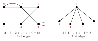
Figure 118: Degrees counted as edge ends. Left: a graph with a pair of multiple edges between the two top-left vertices and a loop at the bottom-right vertex. The bottom-right vertex has degree 4: one end each from the edges to its two neighbours, and two from the loop. The top-middle vertex has degree 5, two of them from the multiple edges. The degrees add to 18, and there are 9 edges. Right: a simple graph, one vertex joined to four others. The centre has degree 4 and each of the others degree 1, a total of 8 for 4 edges.
The Handshake Theorem
The Handshake Theorem. The sum of the degrees of a graph is twice the number of edges. If \(G\) is a graph with \(V(G) = \{v_1, v_2, \dots, v_n\}\) and \(|E(G)| = e\), then \[\sum_{i=1}^{n} \deg(v_i) = 2e.\]
Why. Adding up the degrees counts every edge end in the graph once, at the vertex it touches. Every edge has exactly two ends, an ordinary edge one at each endpoint and a loop both at its one endpoint. So the total number of ends is \(2e\). In the left graph above, 9 edges give 18 ends, and the degrees add to 18.
So the sum of the degrees is always even. That gives the corollary:
Corollary. Every graph has an even number of vertices of odd degree.
Proof. Split the vertices into those of even degree and those of odd degree:
\[2e = \sum_{\deg(v) \text{ even}} \deg(v) \;+\; \sum_{\deg(v) \text{ odd}} \deg(v).\]
The first sum adds even numbers, so it is even. The left side is even. So the second sum, the difference of two even numbers, is even too. It is a sum of odd numbers, and a sum of odd numbers is even only when there is an even number of them. So the number of vertices of odd degree is even. \(\square\)
In the left graph above the odd-degree vertices are the ones of degree 5 and 1, two of them. In the right graph they are the four vertices of degree 1.
The proof of the theorem, and more on degree, are in graphs.
Worked: which statement about degrees is true
Which of the following is true?
(a) In any graph there is an even number of vertices of even degree.
(b) In any graph there is an odd number of vertices of even degree.
(c) In any graph there is an even number of vertices of odd degree.
(d) In any graph there is an odd number of vertices of odd degree.
Answer: (c). It is the corollary of the Handshake Theorem just proved:
\[\sum_{i=1}^{n} \deg(v_i) = \deg(v_1) + \deg(v_2) + \cdots + \deg(v_n) = 2e\]
is even, so the odd degrees among \(\deg(v_1), \dots, \deg(v_n)\) must come in an even number.
Each of the others says “in any graph”, so one graph where it fails is enough to show it is false.
- (a) is false. One vertex joined to four others has degrees \(4, 1, 1, 1, 1\): one vertex of even degree. (A graph with a single vertex and no edges, one vertex of degree 0, also works.)
- (b) is false. Four vertices in a path have degrees \(1, 2, 2, 1\): two vertices of even degree.
- (d) is false. Two vertices joined by one edge have degrees \(1, 1\): two vertices of odd degree. In fact (d) is false for every graph, by (c).
Statements (a) and (b) fail because the number of even-degree vertices can be anything: the corollary controls only the odd ones.
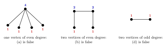
Figure 119: Three graphs that each break one of the false statements. Even degrees are blue and odd degrees red. Left: one vertex joined to four others has just one vertex of even degree, so the number of even-degree vertices need not be even. Middle: a path of four vertices has two vertices of even degree, so it need not be odd either. Right: a single edge has two vertices of odd degree, so the number of odd-degree vertices is not odd. In every graph, as in these three, the red labels come in an even number.
Worked: degree sequences
The list of the degrees of the vertices of a graph is its degree sequence.
For each of the following lists, draw a simple graph with vertices whose degrees are the numbers in the list, or explain why no such graph exists.
(a) 2, 2, 2, 2
(b) 3, 2, 1
(c) 4, 3, 2, 2, 2, 2, 1, 1
(d) 1, 1, 1, 1
(e) 5, 5, 5, 5, 5, 5
Two checks rule a list out straight away:
- The sum must be even, by the Handshake Theorem. Equivalently, the list must contain an even number of odd entries.
- In a simple graph with \(n\) vertices every degree is at most \(n - 1\). With no loops and no multiple edges, a vertex has at most one edge to each of the other \(n - 1\) vertices.
Passing both checks does not guarantee a graph, so for a list that passes, draw one.
| List | Sum | Largest entry vs \(n - 1\) | Simple graph? |
|---|---|---|---|
| (a) 2, 2, 2, 2 | 8 | \(2 \le 3\) | yes: a square, 4 edges |
| (b) 3, 2, 1 | 6 | \(3 > 2\) | no |
| (c) 4, 3, 2, 2, 2, 2, 1, 1 | 17, odd | \(4 \le 7\) | no |
| (d) 1, 1, 1, 1 | 4 | \(1 \le 3\) | yes: two separate edges |
| (e) 5, 5, 5, 5, 5, 5 | 30 | \(5 \le 5\) | yes: every pair of the 6 vertices joined, 15 edges |
- (a) Four vertices around a square, each joined to its two neighbours. Each has degree 2, and \(8 = 2 \cdot 4\) edges.
- (b) There are only three vertices, so in a simple graph a vertex can be joined to at most the other two, and degree 3 is impossible. The sum, 6, is even, so the Handshake Theorem alone does not rule it out. Without the word simple there is a graph: join the degree-3 vertex to the degree-2 vertex by two multiple edges and to the degree-1 vertex by one edge. That graph has multiple edges, so it is not simple.
- (c) The odd entries are 3, 1 and 1, three of them. A graph must have an even number of vertices of odd degree, so no graph exists, simple or not. Equivalently, the sum is 17, which is not \(2e\) for any \(e\).
- (d) Two edges with no vertex in common. Each vertex is the end of one edge.
- (e) Six vertices, every pair joined by an edge. Each vertex is joined to the other 5. There are \(\binom62 = 15\) edges, and \(6 \cdot 5 = 30 = 2 \cdot 15\).
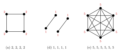
Figure 120: Simple graphs for the three lists that can be realised, each vertex labelled with its degree. (a) 2, 2, 2, 2: a square, each vertex joined to its two neighbours. (d) 1, 1, 1, 1: two edges sharing no vertex. (e) 5, 5, 5, 5, 5, 5: six vertices with every pair joined, 15 edges, so each vertex is joined to all 5 others.
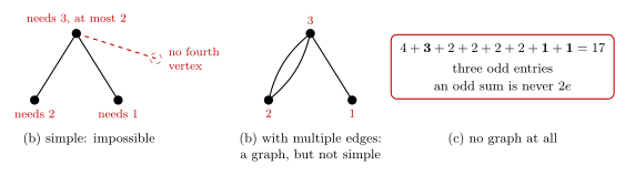
Figure 121: Why lists (b) and (c) have no simple graph. (b) 3, 2, 1: each vertex is labelled with the degree it needs. With three vertices, the vertex that needs degree 3 can be joined to only the 2 others, since a simple graph allows at most one edge to each. A third edge would need a fourth vertex, or a second edge to a vertex it already meets. Allowing multiple edges gives a graph, in the middle, but it is not simple. (c) 4, 3, 2, 2, 2, 2, 1, 1: three entries are odd, and the number of odd-degree vertices in any graph is even.
More on degree sequences, including a list that passes both checks and still has no simple graph, is in graphs.
See also
- pigeonhole-principle — the principle, its generalised form, choosing the holes, and more examples
- [graphs] — graphs, loops and multiple edges, degree, the Handshake Theorem and degree sequences
- 2026-07-27-welcome-and-intro-problems — the five friends with equal friend counts, and the bridges of Königsberg as a graph
- 2026-10-20-inclusion-exclusion — Lecture 32
- practice-problems — §42, with full worked solutions
- practice-problems — §43, with full worked solutions
Week 13
Lecture 34 — Walks, Trails and Circuits
A recap of the graph theory so far (degree, the Handshake Theorem, the pigeonhole argument for equal degrees, complete graphs), then getting around a graph: walks, trails, circuits and connected graphs, and the theorem that says exactly when a graph has an Euler circuit, a circuit using every edge once, or an Euler trail. Pre-work: Video 044 (Walks, Trails and Circuits). Walks, trails, circuits and connectedness are in walks-trails-and-circuits. Euler circuits and trails, the theorem with its proof, how to find one, and the decision flowchart are in euler-circuits-and-trails. The basic definitions are in [graphs].
Goals
- Understand the basic terminology and definitions of graph theory.
- Understand the conditions required for a graph to have an Euler circuit or trail.
Two questions to keep in mind:
- What is the difference between an Euler circuit and an Euler trail? Both use every edge of the graph exactly once. An Euler circuit finishes at the vertex it started from; an Euler trail from \(u\) to \(v\) starts at \(u\) and finishes at a different vertex \(v\). For a connected graph the odd-degree vertices decide which one there is: none gives an Euler circuit, exactly two gives an Euler trail from one to the other, and more gives neither (the theorem).
- How do I actually find an Euler circuit? First decide whether there is one, from the degrees and connectedness (the flowchart). Then build it by splicing: walk along unused edges until stuck, and while edges are left, take a vertex on the route that still has unused edges, walk a circuit from it, and insert that circuit into the route. It is done in full for an Euler trail on ten vertices, and the method, with why it always works, is in euler-circuits-and-trails.
The bridges of Königsberg
The city of Königsberg had four land masses, the north bank \(A\), the island \(B\), the south bank \(C\) and the eastern part \(D\), joined by seven bridges. Is there a walk around the city that crosses every bridge exactly once? As a graph, each land mass is a vertex and each bridge an edge. \(A\) and \(B\) are joined by two bridges, and so are \(B\) and \(C\), so the graph has multiple edges.
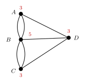
Figure 122: The bridges of Königsberg as a graph: land masses \(A\), \(B\), \(C\), \(D\) as vertices and the seven bridges as edges. Every vertex has odd degree, 3, 5, 3 and 3. An Euler circuit needs every degree even and an Euler trail needs exactly two odd degrees, so there is neither: no walk crosses every bridge exactly once.
The degrees are \(\deg A = 3\), \(\deg B = 5\), \(\deg C = 3\), \(\deg D = 3\), adding to \(14 = 2 \cdot 7\). A walk that crosses every bridge once and comes back is an Euler circuit, and one that finishes on a different land mass from where it started is an Euler trail. By the theorem below the first needs every degree even, and the second needs exactly two odd degrees. Here all four are odd, so neither exists. The problem is set up in 2026-07-27-welcome-and-intro-problems, where the land masses are lettered differently.
Recap: graphs, degree and the Handshake Theorem
All in [graphs]: a graph is a non-empty set of vertices and a possibly empty set of edges, each edge having one or two endpoints (graphs). A loop has one endpoint, multiple edges (parallel edges) share their endpoints, and a graph is simple if it has neither (graphs). The degree of a vertex is the number of edge ends at it, so a loop adds 2: a vertex with two ordinary edges and a loop has degree 4 (graphs). The Handshake Theorem: for a graph with vertices \(v_1, \dots, v_n\) and \(e\) edges, \[\sum_{i=1}^{n} \deg(v_i) = 2e,\] since every edge has two ends (graphs).
Two vertices of the same degree
Theorem. Any simple graph with at least two vertices has two vertices of the same degree.
Proof idea. With \(n\) vertices, a vertex of a simple graph has degree between \(0\) and \(n - 1\). Degrees \(0\) and \(n - 1\) cannot both occur: a vertex of degree \(n - 1\) is adjacent to every other vertex, so none has degree 0. So the degrees all lie in \(\{1, 2, \dots, n - 1\}\) or all lie in \(\{0, 1, \dots, n - 2\}\), at most \(n - 1\) values for \(n\) vertices, and by the pigeonhole principle two vertices share a degree.
For \(n = 6\): if some vertex has degree 5, the degrees are among \(1, 2, 3, 4, 5\); otherwise they are among \(0, 1, 2, 3, 4\). Five values either way, for six vertices. The full proof, with a figure, is in pigeonhole-principle.
Worked: counting with the Handshake Theorem
- A graph has 5 vertices with degree sequence 3, 3, 2, 2, 2. How many edges does the graph have?
- A graph has 6 vertices and 10 edges. If five of its vertices have degree 3, what is the degree of its other vertex?
(a) 6 edges. Let \(e\) be the number of edges. By the Handshake Theorem, \[3 + 3 + 2 + 2 + 2 = 2e, \qquad 12 = 2e, \qquad e = 6.\]
The degree sequence fixes the number of edges, but not the graph. A pentagon with one chord has these degrees and is simple. So does a graph made of three parallel edges between two vertices, two parallel edges between two more, and a loop at the fifth vertex, which is not simple. Both have 6 edges.
(b) Degree 5. Let \(x\) be the degree of the other vertex. By the Handshake Theorem, \[3 + 3 + 3 + 3 + 3 + x = 2 \cdot 10, \qquad 15 + x = 20, \qquad x = 5.\]
Such a graph exists: join one vertex to all five others, and join those five in a ring. Each ring vertex has its two ring neighbours and the centre, degree 3, and the centre has degree 5. That is \(5 + 5 = 10\) edges.
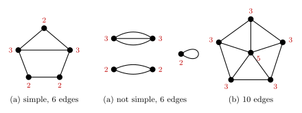
Figure 123: Graphs for the two counting questions, each vertex labelled with its degree. Left: a pentagon with one chord, a simple graph with degrees 3, 3, 2, 2, 2 and 6 edges. Middle: three parallel edges, two parallel edges and a loop, a non-simple graph with the same degrees and also 6 edges. The degree sequence fixes the number of edges, not the graph. Right: one vertex joined to the five vertices of a ring, 10 edges, with the centre of degree 5 and the other five of degree 3.
Complete graphs
In a simple graph there are no loops, and each pair of vertices is joined by at most one edge. There are \(\binom{n}{2}\) pairs of vertices, so a simple graph with \(n\) vertices has at most \(\binom{n}{2}\) edges.
The simple graph with \(n\) vertices and \(\binom{n}{2}\) edges is called the complete graph of order \(n\) and is denoted \(K_n\).
It joins every pair of vertices, so every vertex has degree \(n - 1\). More on these in graphs.
| \(n\) | 1 | 2 | 3 | 4 | 5 | 6 | 7 |
|---|---|---|---|---|---|---|---|
| edges of \(K_n\), \(\binom n2\) | 0 | 1 | 3 | 6 | 10 | 15 | 21 |
| degree of each vertex | 0 | 1 | 2 | 3 | 4 | 5 | 6 |
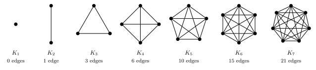
Figure 124: The complete graphs \(K_1\) to \(K_7\). Each joins every pair of its \(n\) vertices once, so it has \(\binom{n}{2}\) edges and every vertex has degree \(n - 1\). Lines cross where there is no vertex; only the dots are vertices.
Walks, trails and circuits
The definitions, in full with examples in walks-trails-and-circuits:
A walk is a sequence \(v_0\, e_1\, v_1\, e_2\, v_2 \cdots e_n\, v_n\) where each \(v_i\) is a vertex and each \(e_i\) is an edge with endpoints \(v_{i-1}\) and \(v_i\).
A trail is a walk where \(e_1, e_2, \dots, e_n\) are pairwise distinct.
A circuit is a trail \(v_0\, e_1\, v_1 \cdots e_n\, v_n\) where \(v_0 = v_n\).
A graph is connected if and only if there is a walk from any given vertex to any other given vertex.
A trail has no repeated edges, but it may repeat vertices. The route below is a trail that passes through one vertex twice.
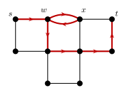
Figure 125: A trail on a graph with two parallel edges at the top. The route, in red, starts at \(s\), goes from \(w\) to \(x\) along one of the parallel edges and back to \(w\) along the other, then goes down and right to finish at \(t\). It passes through \(w\) twice but uses no edge twice, since the two parallel edges are different edges, so it is a trail. It ends at \(t \ne s\), so it is not a circuit. It uses 7 of the 14 edges, so it is not an Euler trail either.
Worked: walks, trails and circuits in \(K_4\)
Determine whether the complete graph \(K_4\) contains the following:
(a) A walk that is not a trail.
(b) A trail that is not a circuit.
(c) An Euler circuit.
Label \(K_4\) with vertices \(v_1, v_2, v_3, v_4\) and edges \(e_1 = v_1v_2\), \(e_2 = v_2v_3\), \(e_3 = v_3v_4\), \(e_4 = v_1v_4\), \(e_5 = v_1v_3\), \(e_6 = v_2v_4\).
(a) Yes. \(v_4\, e_6\, v_2\, e_6\, v_4\, e_4\, v_1\). Each edge joins the vertices on either side of it, so it is a walk. It uses \(e_6\) twice, so it is not a trail.
(b) Yes. \(v_1\, e_4\, v_4\). A single edge is a trail, since no edge is repeated, and it ends at \(v_4 \ne v_1\), so it is not a circuit.
(c) No. \(K_4\) is connected, but every vertex has degree 3, which is odd, so by the theorem there is no Euler circuit. In fact there is no Euler trail either: that needs exactly two vertices of odd degree, and \(K_4\) has four.
Other answers work for (a) and (b). Any route that goes out and back along one edge answers (a), and any trail that ends somewhere other than its start answers (b), for example \(v_1\, e_1\, v_2\, e_2\, v_3\, e_5\, v_1\, e_4\, v_4\), which repeats \(v_1\) but no edge.
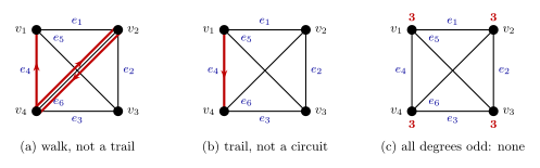
Figure 126: The three parts on \(K_4\). (a) The walk \(v_4,e_6,v_2,e_6,v_4,e_4,v_1\): the doubled red line is \(e_6\) used twice, so it is a walk but not a trail. (b) The trail \(v_1,e_4,v_4\): one edge, no repeats, and it ends at a different vertex from where it started. (c) Every vertex of \(K_4\) has degree 3, odd, so there is no Euler circuit, and with four odd vertices no Euler trail either.
Euler circuits and Euler trails
An Euler circuit is a circuit that contains every edge of the graph.
An Euler trail from vertex \(u\) to vertex \(v\) is a trail that starts at \(u\) and ends at \(v\) and contains every edge of the graph.
A graph with an Euler circuit is called Eulerian.
Theorem. Let \(G\) be a connected graph. Then \(G\) has an Euler circuit if and only if every vertex of \(G\) has even degree. Let \(u, v \in V(G)\) be distinct vertices of \(G\). Then \(G\) has an Euler trail from \(u\) to \(v\) if and only if \(u\) and \(v\) have odd degree and all other vertices of \(G\) have even degree.
Why the degrees. Each time a route passes through a vertex it arrives along one edge and leaves along another, using two edge ends there. If the route uses every edge exactly once, it uses every edge end at a vertex, so the degree is twice the number of passes, which is even. The exceptions are the start and the end: a trail from \(u\) to \(v \ne u\) leaves \(u\) once without having arrived and arrives at \(v\) once without leaving, so those two have odd degree. For a circuit the start and end are the same vertex and pair up. The other direction, that the right degrees guarantee an Euler circuit or trail when the graph is connected, is proved by building one, in euler-circuits-and-trails.
This course uses the standard definitions above. The textbook defines an Euler circuit as a circuit that contains every vertex and every edge. For connected graphs the two agree. In a connected graph with at least one edge every vertex is the endpoint of some edge, so a route using every edge passes through every vertex. A connected graph with no edges is a single vertex, and the trivial circuit there contains it. They differ when there are isolated vertices.

Figure 127: A square and an isolated vertex in the middle. Going once round the square, in red, is a circuit that contains every edge, so by this course’s definition the graph has an Euler circuit. By the textbook’s definition, which also asks for every vertex, it does not, since no circuit reaches the middle vertex.
More on the two definitions, with the proof that they agree for connected graphs, is in euler-circuits-and-trails.
Worked: which graphs have an Euler circuit or trail
For each of the following graphs, determine whether the graph has an Euler circuit. For those that do not contain an Euler circuit, determine whether the graph has an Euler trail.
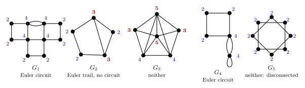
Figure 128: The five graphs, each vertex labelled with its degree, odd degrees in red. \(G_1\) has two parallel edges at the top, and in \(G_4\) the bottom vertex has two parallel edges and a loop, which adds 2. \(G_1\) and \(G_4\) are connected with every degree even, so they have Euler circuits. \(G_2\) has exactly two odd vertices, so it has an Euler trail between them. \(G_3\) has four odd vertices, so it has neither. In \(G_5\) every degree is even, but the graph is two separate squares, since the crossings are not vertices, so it has neither.
| Graph | Degrees | Connected? | Odd vertices | Verdict |
|---|---|---|---|---|
| \(G_1\) | 2, 4, 4, 2 (top), 2, 4, 4, 2 (middle), 2, 2 (bottom) | yes | none | Euler circuit |
| \(G_2\) | 3, 2, 2, 2, 3 | yes | two | no Euler circuit; Euler trail |
| \(G_3\) | 5, 3, 3, 5, 4, 4 | yes | four | neither |
| \(G_4\) | 2, 2, 2, 4, 4 | yes | none | Euler circuit |
| \(G_5\) | 2 for all eight | no | none | neither |
- \(G_1\). 14 edges, degrees adding to 28. Every degree is even and the graph is connected, so it has an Euler circuit. The two parallel edges at the top each count once at each end, which is why those two vertices have degree 4.
- \(G_2\). A pentagon with a chord. The two ends of the chord have degree 3 and the rest degree 2. Exactly two odd vertices, so there is no Euler circuit, but there is an Euler trail from one end of the chord to the other: start at the top vertex, go all the way round the pentagon back to the top, then take the chord down.
- \(G_3\). 12 edges. The top vertex and the centre each have degree 5, the left and right vertices degree 3, and the bottom two degree 4. Four odd vertices: no Euler circuit and no Euler trail.
- \(G_4\). 7 edges: the square, the two parallel edges and the loop. The loop adds 2, so the bottom vertex has degree \(2 + 2 = 4\), and the square’s bottom-right corner has degree 4 too. All even and connected, so there is an Euler circuit: round the square, down one parallel edge, round the loop, back up the other.
- \(G_5\). Every degree is 2, so the degrees alone would suggest an Euler circuit. But the lines cross at points that are not vertices, and the graph is two separate squares, an upright one and a tilted one. It is not connected, and a single route cannot use edges in both pieces, so there is no Euler circuit and no Euler trail. The theorem only applies to connected graphs.
Worked: an Euler trail from \(a\) to \(e\)
Use the theorem to show that the graph below has an Euler trail from \(a\) to \(e\), and find one.
The graph has 21 edges: \(ab\), \(ah\), \(ai\), \(bc\), \(bd\), \(bh\), \(cd\), \(cf\), \(ci\), \(de\), \(df\), \(ef\), \(fg\), \(fi\), \(fj\), \(gh\), \(gi\), \(gj\), \(hi\), \(ij\), \(je\). The graph is simple, so a route can be written as a list of vertices.
| Vertex | \(a\) | \(b\) | \(c\) | \(d\) | \(e\) | \(f\) | \(g\) | \(h\) | \(i\) | \(j\) |
|---|---|---|---|---|---|---|---|---|---|---|
| Degree | 3 | 4 | 4 | 4 | 3 | 6 | 4 | 4 | 6 | 4 |
The degrees add to \(42 = 2 \cdot 21\). Vertices \(a\) and \(e\) have odd degree, all other vertices have even degree, and the graph is connected, so by the theorem it has an Euler trail from \(a\) to \(e\).
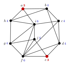
Figure 129: The graph on \(a\) to \(j\), each vertex labelled with its degree. Only \(a\) and \(e\), in red, have odd degree, and the graph is connected, so there is an Euler trail from \(a\) to \(e\) and no Euler circuit. Lines cross at several points that are not vertices.
Finding one by splicing. Start at \(a\), one of the two odd vertices, and walk along unused edges until stuck:
\[a,\ b,\ c,\ d,\ e,\ f,\ j,\ e.\]
At \(e\) all three edges are now used, so this is stuck, at \(e\) as it must be. It uses 7 of the 21 edges. The 14 unused edges give every vertex even degree, and \(j\) is on the route and still has unused edges (\(ji\) and \(jg\)). Walk from \(j\) along unused edges until stuck, which brings it back to \(j\):
\[j,\ i,\ c,\ f,\ i,\ a,\ h,\ i,\ g,\ h,\ b,\ d,\ f,\ g,\ j.\]
That uses the other 14 edges. Insert it into the first route at \(j\):
\[a,\ b,\ c,\ d,\ e,\ f,\ \underbrace{j,\ i,\ c,\ f,\ i,\ a,\ h,\ i,\ g,\ h,\ b,\ d,\ f,\ g,\ j}_{\text{inserted}},\ e.\]
This is an Euler trail from \(a\) to \(e\): 21 edges, each of the 21 exactly once, starting at \(a\) and ending at \(e\). It passes through \(f\) and \(i\) three times each, using all six edges at each.
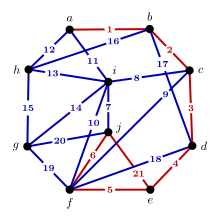
Figure 130: The Euler trail from \(a\) to \(e\), with each edge numbered in the order the trail uses it. Red: the first walk from \(a\), which gets stuck at \(e\) after 7 edges. Blue: the circuit from \(j\) through the 14 unused edges, inserted into the first walk at \(j\), between edges 6 and 21. Following the numbers 1 to 21 gives \(a,b,c,d,e,f,j,i,c,f,i,a,h,i,g,h,b,d,f,g,j,e\).
The trail is not unique. Walking differently until stuck, or inserting at a different vertex, gives other Euler trails from \(a\) to \(e\), and reversing any of them gives an Euler trail from \(e\) to \(a\).
Deciding: the flowchart
How to tell whether a graph has an Euler circuit, connected or not:
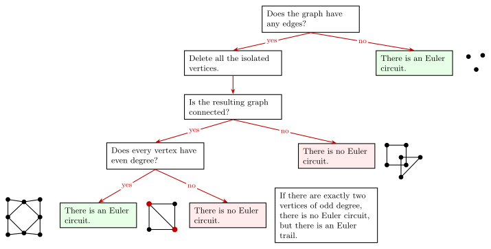
Figure 131: Deciding whether a graph has an Euler circuit, with an example graph at each outcome. No edges: the trivial circuit counts, as for three isolated vertices. Otherwise delete the isolated vertices and check that what is left is connected. A square and a triangle that only cross in the drawing are two pieces, so there is no Euler circuit even though every degree is even. Then check the degrees: the eight-vertex graph has degrees 2 and 4 and has an Euler circuit, while the square with one diagonal has two vertices of degree 3, so it has no Euler circuit but does have an Euler trail.
Each step, in words:
- No edges at all. Then there is an Euler circuit: the trivial circuit, a single vertex, contains every edge, since there are none.
- Delete the isolated vertices. A route never needs to visit a vertex with no edges, and this course’s definition only asks for every edge.
- Not connected. Two edges in different pieces cannot be on one route, so there is no Euler circuit, and no Euler trail either.
- Connected. The theorem decides: every degree even gives an Euler circuit. Otherwise there is no Euler circuit, and if there are exactly two vertices of odd degree, there is an Euler trail from one to the other.
A version that also sorts out the Euler trail case completely, with why each step is right, is in euler-circuits-and-trails.
See also
- walks-trails-and-circuits — walks, trails, circuits, trivial circuits, circuit-free and connected graphs
- euler-circuits-and-trails — the theorem with a full proof, how to find an Euler circuit or trail, the flowchart, and the textbook’s definition
- [graphs] — degree, the Handshake Theorem and complete graphs
- pigeonhole-principle — two vertices of equal degree in a simple graph
- 2026-07-27-welcome-and-intro-problems — the bridges of Königsberg, first posed
- 2026-10-22-pigeonhole-principle-introduction-to-graph-theory — Lecture 33
- 2026-10-27-matrix-representations-of-graphs — Lecture 35
- practice-problems — §44, with full worked solutions
Lecture 35 — Matrix Representations of Graphs
Two ways to write a graph down as a table of numbers. The adjacency matrix has a row and a column for each vertex and records how many edges join each pair of vertices. The incidence matrix has a row for each vertex and a column for each edge and records how many times each vertex is incident with each edge. Both go in both directions: a graph gives a matrix, and a matrix of the right kind gives a graph. Pre-work: Video 045 (Matrix Representations of Graphs). The definitions, how loops are counted, reading a graph off a matrix and which matrices qualify are in adjacency-matrices and incidence-matrices. Graphs, degree and the Handshake Theorem are in [graphs].
Goals
- Learn how to represent a graph by an adjacency matrix.
- Learn how to represent a graph by an incidence matrix.
- Learn how to draw a graph from its adjacency matrix.
- Learn how to draw a graph from its incidence matrix.
Two questions to keep in mind:
- In an incidence matrix, which are the rows and which are the columns: the vertices or the edges? The vertices are the rows and the edges are the columns, as in the definition. There is a way to remember it in which way round.
- Is it OK to swap them? The swapped matrix holds the same information, but it is not the incidence matrix as this course defines it. Also in which way round.
The running example
One graph is used all the way through. It has vertex set \(\{v_1, v_2, v_3, v_4\}\) and edge set \(\{e_1, e_2, e_3, e_4, e_5\}\), with
| Edge | Endpoints |
|---|---|
| \(e_1\) | \(\{v_2, v_3\}\) |
| \(e_2\) | \(\{v_2, v_3\}\) |
| \(e_3\) | \(\{v_1, v_2\}\) |
| \(e_4\) | \(\{v_1, v_4\}\) |
| \(e_5\) | \(\{v_4\}\) |
So \(e_1\) and \(e_2\) are parallel edges, and \(e_5\) is a loop at \(v_4\). The degrees are \(\deg(v_1) = 2\), \(\deg(v_2) = 3\), \(\deg(v_3) = 2\) and \(\deg(v_4) = 3\), the loop adding 2 to \(\deg(v_4)\). They add to \(10 = 2 \cdot 5\).
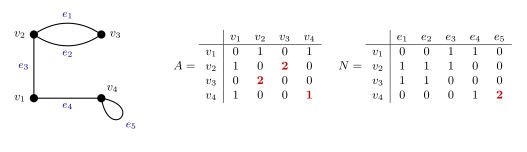
Figure 132: The running example and its two matrices. The adjacency matrix A has a row and a column for each vertex, and each entry counts the edges joining that pair of vertices: the 2 is the pair of parallel edges between v2 and v3, and the 1 on the diagonal is the single loop at v4. The incidence matrix N has a row for each vertex and a column for each edge, and each entry counts how many times that vertex is incident with that edge: the 2 is the loop, which meets v4 at both of its ends.
Worked: edges between pairs of vertices
For the running example, how many edges have the following as endpoints?
(a) \(\{v_1, v_2\}\)
(b) \(\{v_1, v_3\}\)
(c) \(\{v_1, v_4\}\)
(d) \(\{v_2, v_3\}\)
(e) \(\{v_4\}\)
| Endpoints | Edges | Number | |
|---|---|---|---|
| (a) | \(\{v_1, v_2\}\) | \(e_3\) | 1 |
| (b) | \(\{v_1, v_3\}\) | none | 0 |
| (c) | \(\{v_1, v_4\}\) | \(e_4\) | 1 |
| (d) | \(\{v_2, v_3\}\) | \(e_1\), \(e_2\) | 2 |
| (e) | \(\{v_4\}\) | \(e_5\) | 1 |
For (e), the set of endpoints \(\{v_4\}\) has one element, so the edges with that set of endpoints are the loops at \(v_4\). There is one, \(e_5\).
These five numbers are entries of the adjacency matrix. Answers (a), (b) and (c), with a 0 for “no loop at \(v_1\)”, are the first row, \(0\ 1\ 0\ 1\). Answer (d) is the entry in row \(v_2\), column \(v_3\), and answer (e) is the diagonal entry in row \(v_4\), column \(v_4\).
The adjacency matrix
The adjacency matrix of a graph with vertices \(v_1, v_2, \dots, v_n\) is the \(n \times n\) matrix \(A = [a_{ij}]\) where each entry \(a_{ij}\) is the number of edges with endpoints \(\{v_i, v_j\}\).
When \(i = j\) the set \(\{v_i, v_i\}\) is just \(\{v_i\}\), so a diagonal entry \(a_{ii}\) is the number of loops at \(v_i\). A loop is one edge, so it counts 1 on the diagonal. In the running example \(a_{44} = 1\) for the single loop \(e_5\).
Three things follow straight from the definition:
- \(\{v_i, v_j\} = \{v_j, v_i\}\), so \(a_{ij} = a_{ji}\): the matrix is symmetric.
- Every entry counts edges, so every entry is a non-negative integer.
- A loop adds 2 to a degree but only 1 to the matrix. So \(\deg(v_i)\) is the row sum plus the diagonal entry. In the running example row \(v_4\) adds to \(1 + 0 + 0 + 1 = 2\), and \(\deg(v_4) = 2 + a_{44} = 3\).
More on all three, and the proofs, in adjacency-matrices.
Worked: write down the adjacency matrix
Write down the adjacency matrix for the graph below.
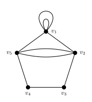
Figure 133: The graph for the first question: five vertices around a pentagon, two loops at v1, and two parallel edges between v5 and v2. It has 9 edges in all.
Answer.
\[A = \begin{array}{c|ccccc} & v_1 & v_2 & v_3 & v_4 & v_5 \\ \hline v_1 & 2 & 1 & 0 & 0 & 1 \\ v_2 & 1 & 0 & 1 & 0 & 2 \\ v_3 & 0 & 1 & 0 & 1 & 0 \\ v_4 & 0 & 0 & 1 & 0 & 1 \\ v_5 & 1 & 2 & 0 & 1 & 0 \end{array}\]
Go through the pairs once each, then copy across the diagonal, since the matrix is symmetric.
- Diagonal. Two loops at \(v_1\), so \(a_{11} = 2\). No other vertex has a loop.
- Row \(v_1\). One edge to \(v_2\), one to \(v_5\), none to \(v_3\) or \(v_4\).
- Row \(v_2\). One edge to \(v_3\) and two parallel edges to \(v_5\), so \(a_{25} = 2\).
- Rows \(v_3\) and \(v_4\). One edge \(v_3 v_4\) and one edge \(v_4 v_5\).
Two checks.
- Edge count. Each edge is counted once in the upper triangle with the diagonal: \((2 + 1 + 0 + 0 + 1) + (0 + 1 + 0 + 2) + (0 + 1 + 0) + (0 + 1) + 0 = 4 + 3 + 1 + 1 + 0 = 9\), the 9 edges of the graph.
- Degrees. Row sum plus diagonal entry: \(\deg(v_1) = 4 + 2 = 6\), the two loops giving 4 of it, and \(\deg(v_2) = 4\), \(\deg(v_3) = 2\), \(\deg(v_4) = 2\), \(\deg(v_5) = 4\). They add to \(18 = 2 \cdot 9\), as the graphs says they must.
Worked: draw the graph of an adjacency matrix
Draw the graph with this adjacency matrix. \[\begin{array}{c|ccccc} & v_1 & v_2 & v_3 & v_4 & v_5 \\ \hline v_1 & 2 & 1 & 0 & 3 & 1 \\ v_2 & 1 & 0 & 0 & 0 & 2 \\ v_3 & 0 & 0 & 0 & 1 & 0 \\ v_4 & 3 & 0 & 1 & 0 & 1 \\ v_5 & 1 & 2 & 0 & 1 & 0 \end{array}\]
First check that it can be an adjacency matrix: it is square, symmetric and its entries are non-negative integers. Then read only the diagonal and the entries above it. Each entry below the diagonal repeats one above it, and reading both would draw every edge twice.
| Entry | Value | Edges |
|---|---|---|
| \(a_{11}\) | 2 | two loops at \(v_1\) |
| \(a_{12}\) | 1 | one edge \(v_1 v_2\) |
| \(a_{14}\) | 3 | three parallel edges \(v_1 v_4\) |
| \(a_{15}\) | 1 | one edge \(v_1 v_5\) |
| \(a_{25}\) | 2 | two parallel edges \(v_2 v_5\) |
| \(a_{34}\) | 1 | one edge \(v_3 v_4\) |
| \(a_{45}\) | 1 | one edge \(v_4 v_5\) |
Every other entry on or above the diagonal is 0. That is \(2 + 1 + 3 + 1 + 2 + 1 + 1 = 11\) edges.
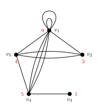
Figure 134: The graph drawn from the matrix: two loops at v1, three parallel edges between v1 and v4, two between v2 and v5, and single edges v1v2, v1v5, v3v4 and v4v5. The three v1v4 edges cross the two v2v5 edges, but crossings are not vertices. The degrees, in red, are each row sum plus the diagonal entry, so v1 has degree 7 + 2 = 9. They add to 22, twice the 11 edges.
The degrees are \(\deg(v_1) = 7 + 2 = 9\), \(\deg(v_2) = 3\), \(\deg(v_3) = 1\), \(\deg(v_4) = 5\) and \(\deg(v_5) = 4\), a total of \(22 = 2 \cdot 11\). Where the vertices go on the page is free. The matrix fixes only which vertices are joined, and how many times.
Worked: which is an adjacency matrix
Which of the following is an adjacency matrix for a graph?
A. \(\begin{bmatrix} 1 & 0 \\ 0 & -1 \end{bmatrix}\)
B. \(\begin{bmatrix} 1 & 1 & 1 \\ 1 & 1 & 1 \end{bmatrix}\)
C. \(\begin{bmatrix} 73 \end{bmatrix}\)
D. \(\begin{bmatrix} 0 & 1 & 0 & 1 \\ 1 & 0 & 2 & 2 \\ 0 & 2 & 0 & 0 \\ 1 & 1 & 0 & 1 \end{bmatrix}\)
Answer: C.
A matrix is an adjacency matrix of some graph exactly when it is square, symmetric and has non-negative integer entries (adjacency-matrices).
- A is square and symmetric, but \(-1\) cannot be a number of edges.
- B is \(2 \times 3\). An adjacency matrix has one row and one column for each vertex, so it is always square.
- C is \(1 \times 1\), trivially symmetric, and 73 is a non-negative integer. It is the graph with one vertex and 73 loops. That vertex has degree \(73 + 73 = 146\), and the graph has 73 edges.
- D is square with non-negative integer entries, but not symmetric: \(a_{24} = 2\) and \(a_{42} = 1\). The number of edges between \(v_2\) and \(v_4\) cannot be both 2 and 1. Every other pair matches across the diagonal; this one pair is enough.
Figure 135: The graph of the 1 by 1 matrix [73]: a single vertex with 73 loops, three of them drawn and the dashed one standing for the rest. Its one diagonal entry counts the loops, 73, and its degree is twice that, 146.
Worked: how many times is a vertex incident with an edge
For the running example:
(a) How many times is \(v_1\) incident with \(e_1\)?
(b) How many times is \(v_1\) incident with \(e_4\)?
(c) How many times is \(v_2\) incident with \(e_2\)?
(d) How many times is \(v_4\) incident with \(e_5\)?
(a) 0. The endpoints of \(e_1\) are \(v_2\) and \(v_3\), so \(e_1\) does not meet \(v_1\).
(b) 1. \(e_4\) joins \(v_1\) and \(v_4\). One of its ends is at \(v_1\).
(c) 1. \(e_2\) joins \(v_2\) and \(v_3\). One of its ends is at \(v_2\).
(d) 2. \(e_5\) is a loop at \(v_4\). Both of its ends are at \(v_4\), so it meets \(v_4\) twice. This is the same count that makes a loop add 2 to a degree (graphs).
The incidence matrix
The incidence matrix of a graph with vertices \(v_1, v_2, \dots, v_n\) and edges \(e_1, e_2, \dots, e_m\) is the \(n \times m\) matrix \(N = [n_{ij}]\) where each entry \(n_{ij}\) is the number of times vertex \(v_i\) is incident with edge \(e_j\).
The answers above are four of its entries: \(n_{11} = 0\), \(n_{14} = 1\), \(n_{22} = 1\) and \(n_{45} = 2\). The whole matrix for the running example is in the figure.
- A column is an edge. It has a 1 at each of the edge’s two endpoints, or a single 2 at the vertex of a loop. Either way every column adds to 2: every edge has two ends.
- A row is a vertex. It adds up the ends of edges at that vertex, so the row sum is the degree, loops included. In the running example the rows add to \(2, 3, 2, 3\).
- Parallel edges are identical columns. The columns of \(e_1\) and \(e_2\) are both \((0, 1, 1, 0)\).
Adding up all the entries by columns gives \(2m\), and by rows gives the sum of the degrees. That is the graphs again. More in incidence-matrices.
Which way round
Rows are vertices, columns are edges. One way to remember it: the entry \(n_{ij}\) answers “how many times is vertex \(v_i\) incident with edge \(e_j\)”, and the index that comes first, \(i\), is the row, so the vertex comes first. Another: the adjacency matrix has a row for each vertex, and so does the incidence matrix. Both matrices have \(n\) rows, one per vertex; they differ only in their columns, vertices for \(A\) and edges for \(N\).
Swapping them gives the transpose \(N^{\mathsf T}\), the \(m \times n\) matrix with a row for each edge. It holds exactly the same information. The graph can be rebuilt from it just as well, with every row adding to 2 and every column adding to a degree. But it is not the incidence matrix as this course defines it. When asked for the incidence matrix, put the vertices down the side and the edges across the top, and label both.
The question does not arise for the adjacency matrix, because it is symmetric: swapping rows and columns gives the same matrix. What does matter for both is the order of the vertices, and for \(N\) the order of the edges. A different order permutes the rows or columns and gives a different matrix for the same graph, which is why the rows and columns should always be labelled.
Worked: write down the incidence matrix
Write down the incidence matrix for the graph below.
Figure 136: The graph for the incidence-matrix question: a loop e1 at v1, two parallel edges e2 and e3 between v5 and v2, an edge e4 from v5 to v4, and an isolated vertex v3. The loop gives v1 the entry 2 in column e1, and v3, which meets no edge, gives a row of zeros.
Answer.
\[N = \begin{array}{c|cccc} & e_1 & e_2 & e_3 & e_4 \\ \hline v_1 & 2 & 0 & 0 & 0 \\ v_2 & 0 & 1 & 1 & 0 \\ v_3 & 0 & 0 & 0 & 0 \\ v_4 & 0 & 0 & 0 & 1 \\ v_5 & 0 & 1 & 1 & 1 \end{array}\]
Fill it one column, one edge, at a time.
- \(e_1\) is a loop at \(v_1\): a 2 in row \(v_1\) and 0 elsewhere.
- \(e_2\) and \(e_3\) both join \(v_5\) and \(v_2\): a 1 in rows \(v_2\) and \(v_5\). Being parallel, they give the same column.
- \(e_4\) joins \(v_5\) and \(v_4\): a 1 in rows \(v_4\) and \(v_5\).
Checks. Every column adds to 2. The row sums are the degrees, \(2, 2, 0, 1, 3\), adding to \(8 = 2 \cdot 4\). The row of \(v_3\) is all zeros, because \(v_3\) is isolated: a vertex still gets its row even when no edge meets it.
Worked: draw the graph of an incidence matrix
Draw the graph with this incidence matrix. \[\begin{array}{c|cccc} & e_1 & e_2 & e_3 & e_4 \\ \hline v_1 & 2 & 1 & 0 & 0 \\ v_2 & 0 & 1 & 0 & 0 \\ v_3 & 0 & 0 & 2 & 0 \\ v_4 & 0 & 0 & 0 & 1 \\ v_5 & 0 & 0 & 0 & 1 \end{array}\]
Every column adds to 2, so it is an incidence matrix. Read it one column at a time. A column with two 1s is an edge between those two vertices, and a column with a single 2 is a loop.
| Column | Entries | Edge |
|---|---|---|
| \(e_1\) | 2 at \(v_1\) | loop at \(v_1\) |
| \(e_2\) | 1 at \(v_1\), 1 at \(v_2\) | \(v_1 v_2\) |
| \(e_3\) | 2 at \(v_3\) | loop at \(v_3\) |
| \(e_4\) | 1 at \(v_4\), 1 at \(v_5\) | \(v_4 v_5\) |
Figure 137: The graph drawn from the incidence matrix: each column is one edge. Columns e1 and e3 each have a single 2, so they are loops, at v1 and at v3. Columns e2 and e4 each have two 1s, so they join v1 to v2 and v4 to v5. The graph falls into three pieces. The row sums 3, 1, 2, 1, 1 are the degrees, and add to 8, twice the 4 edges.
Worked: which is an incidence matrix
Which of the following is an incidence matrix for a graph?
A. \(\begin{bmatrix} 1 & 0 \\ 0 & 3 \end{bmatrix}\)
B. \(\begin{bmatrix} 1 & 1 & 1 \\ 1 & 1 & 1 \end{bmatrix}\)
C. \(\begin{bmatrix} 1 & 0 \\ 0 & 1 \end{bmatrix}\)
D. \(\begin{bmatrix} 0 & 1 & 0 & 1 \\ 1 & 0 & 2 & 2 \\ 0 & 2 & 0 & 0 \\ 1 & 1 & 0 & 1 \end{bmatrix}\)
Answer: B.
A matrix is an incidence matrix of some graph exactly when its entries are non-negative integers and every column adds to 2, so that each column is either two 1s or a single 2 (incidence-matrices). Check the columns.
| Column sums | Verdict | |
|---|---|---|
| A | \(1,\ 3\) | no: the first column is an edge with one end, and no vertex can meet an edge 3 times |
| B | \(2,\ 2,\ 2\) | yes |
| C | \(1,\ 1\) | no: each column is an edge with only one end |
| D | \(2,\ 4,\ 2,\ 4\) | no: columns 2 and 4 would be edges with four ends |
B has two rows and three columns, so two vertices and three edges, and each column \((1, 1)\) is an edge joining the two vertices. It is two vertices joined by three parallel edges.
In C a column with a single 1 is not a loop: a loop meets its vertex twice and is a single 2. In D the first and third columns are fine on their own, an edge \(v_2 v_4\) and a loop at \(v_2\), but one bad column is enough to rule a matrix out. A square shape, or symmetry, has nothing to do with it: B is not square, and C is square and symmetric.
Figure 138: The graph of matrix B: two vertices and three edges. Each column of B is (1, 1), a 1 at each vertex, so each edge joins v1 and v2. The three columns are identical, which is exactly what three parallel edges look like in an incidence matrix.
Worked: Eulerian from the incidence matrix
For each of the following incidence matrices, determine whether the associated graph \(G\) is Eulerian. Explain why or why not. \[\text{(a)}\ \ N = \begin{array}{c|cccccc} & e_1 & e_2 & e_3 & e_4 & e_5 & e_6 \\ \hline v_1 & 1 & 1 & 0 & 0 & 0 & 0 \\ v_2 & 1 & 0 & 1 & 1 & 0 & 1 \\ v_3 & 0 & 1 & 1 & 0 & 1 & 1 \\ v_4 & 0 & 0 & 0 & 1 & 1 & 0 \end{array} \qquad \text{(b)}\ \ N = \begin{array}{c|cccc} & a & b & c & d \\ \hline u & 1 & 0 & 1 & 0 \\ v & 0 & 1 & 0 & 1 \\ w & 0 & 1 & 0 & 1 \\ x & 1 & 0 & 1 & 0 \end{array}\]
A graph is Eulerian if it has an Euler circuit, a circuit that contains every edge (euler-circuits-and-trails). The test is the theorem (euler-circuits-and-trails):
A connected graph has an Euler circuit if and only if every vertex has even degree.
The incidence matrix gives both halves of the test. The degrees are the row sums, and the columns say which vertices each edge joins, which settles whether the graph is connected.
(a) Yes, \(G\) is Eulerian.
The row sums give the degrees:
\[\deg(v_1) = 2, \quad \deg(v_2) = 4, \quad \deg(v_3) = 4, \quad \deg(v_4) = 2.\]
All four are even. Reading the columns, the edges are \(e_1 = v_1 v_2\), \(e_2 = v_1 v_3\), \(e_3 = v_2 v_3\), \(e_4 = v_2 v_4\), \(e_5 = v_3 v_4\) and \(e_6 = v_2 v_3\), so \(e_3\) and \(e_6\) are parallel. \(G\) is connected: \(v_2\) is joined to each of \(v_1\), \(v_3\) and \(v_4\). A connected graph with every degree even has an Euler circuit, for example
\[v_1\ e_1\ v_2\ e_3\ v_3\ e_6\ v_2\ e_4\ v_4\ e_5\ v_3\ e_2\ v_1.\]
It uses \(e_1, e_3, e_6, e_4, e_5, e_2\), each of the six edges exactly once, each edge joins the vertices on either side of it in the list, and it ends where it started.
(b) No, \(G\) is not Eulerian.
Every row adds to 2, so every vertex has even degree. But the columns show the edges are \(a = ux\), \(b = vw\), \(c = ux\) and \(d = vw\). No edge joins \(u\) or \(x\) to \(v\) or \(w\), so \(G\) is not connected: it is two separate pieces, \(u\) and \(x\) joined by \(a\) and \(c\), and \(v\) and \(w\) joined by \(b\) and \(d\). A circuit is a walk, and a walk only moves along edges, so it never leaves the piece it starts in. No circuit can contain both \(a\) and \(b\), so there is no Euler circuit. Even degrees are not enough on their own: the theorem needs the graph to be connected.
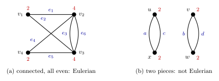
Figure 139: The two graphs read off the incidence matrices, degrees in red. Left, (a): every degree is even and the graph is connected, so it has an Euler circuit; the diagonals e2 and e4 cross without meeting. Right, (b): every degree is 2, but the graph is two separate pieces, and a circuit cannot get from one piece to the other, so no circuit uses every edge.
See also
- adjacency-matrices — the definition, loops on the diagonal, reading a graph off, and which matrices are adjacency matrices
- incidence-matrices — the definition, column sums and row sums, reading a graph off, which matrices qualify, and how the two matrices compare
- [graphs] — loops, parallel edges, degree and the Handshake Theorem
- euler-circuits-and-trails — Euler circuits and trails and the even-degree theorem
- walks-trails-and-circuits — walks, circuits and connected graphs
- 2026-10-26-walks-trails-and-circuits — Lecture 34
- 2026-10-29-trees — Lecture 36
- practice-problems — §45, with full worked solutions
Lecture 36 — Trees
Trees: connected graphs with no non-trivial circuits. The topics are trivial and non-trivial circuits, circuit-free graphs, the definition of a tree, what happens when an edge is deleted from a tree, and the main theorem: a graph with \(n\) vertices is a tree if and only if it is simple, connected and has \(n - 1\) edges. That theorem together with the Handshake Theorem answers most counting questions about trees, as in the four worked questions. Pre-work: Video 046 (Trees). The definitions, the theorem, vertices of degree 1 and the counting method are collected in [trees]. Walks, trails, circuits and connectedness are in walks-trails-and-circuits, and degree and the Handshake Theorem in [graphs].
Trees are the last topic of the course. For exam revision there is a high-level summary of the course topics, and review sessions for the final exam run the following week.
Goals
- Understand the definition and properties of trees.
- Gain fluency in graph theory proofs.
Trivial and non-trivial circuits
A circuit is a trail \(v_0 e_1 v_1 e_2 \cdots e_n v_n\) with \(v_0 = v_n\): a walk that ends where it starts and never uses an edge twice (walks-trails-and-circuits). Nothing in that definition stops \(n = 0\), so a single vertex on its own is a circuit.
A trivial circuit is a circuit consisting of a single vertex and no edges.
A non-trivial circuit is a circuit that has edges.
A graph is circuit-free if there are no non-trivial circuits.
Every vertex is a trivial circuit, so every graph has circuits. That is why circuit-free asks only about the circuits that have edges.
The smallest non-trivial circuits:
- A loop. A loop \(e\) at \(v\) gives the circuit \(v\,e\,v\), with one edge.
- Two multiple edges. If \(e_1\) and \(e_2\) both join \(u\) and \(v\), then \(u\,e_1\,v\,e_2\,u\) is a circuit: it ends where it starts, and its two edges are different.
So a circuit-free graph has no loops and no multiple edges: it is simple.
A circuit can pass through a vertex more than once. Only its edges cannot repeat.
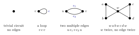
Figure 140: Left: a single vertex is a trivial circuit, a circuit with no edges. The other three are non-trivial circuits. A loop at \(v\) is the circuit \(v,e,v\). Two edges joining \(u\) and \(v\) make the circuit \(u,e_1,v,e_2,u\), which is why a circuit-free graph has no multiple edges. The circuit on the right, \(w,a,b,w,c,d,w\), visits \(w\) twice but uses each of its six edges once, so it is still a circuit.
Trees
Definition. A graph is a tree if and only if it is connected and circuit-free.
A single vertex is a tree: it is connected, and with no edges it has no non-trivial circuit. So is a single edge, and so is one vertex joined to three others. A triangle is connected but is a circuit, so it is not a tree. Two edges with no vertex in common are circuit-free but not connected, so that is not a tree either. And by the last section, every tree is simple.
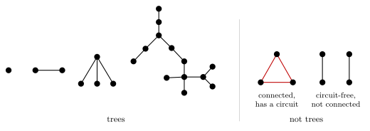
Figure 141: Left: four trees, a single vertex, a single edge, one vertex joined to three others, and a larger tree with 13 vertices. Each is connected, and none has a circuit with edges. Right: two graphs that are not trees. The triangle is connected but is itself a non-trivial circuit, in red. The two separate edges have no circuit, but there is no walk from one edge to the other, so the graph is not connected.
The 11 trees with 7 vertices
There are 11 essentially different trees with 7 vertices. Essentially different means different in shape, not just in the names of the vertices or in how the tree is drawn. Two graphs are isomorphic when one can be turned into the other by renaming its vertices: there is a way to match the vertices of one with the vertices of the other so that two vertices are joined in the first exactly when the matching vertices are joined in the second. Isomorphic graphs are the same graph with different labels, and count once. If the 7 vertices are named and two trees count as different whenever their edge sets differ, there are far more of them: \(7^5 = 16807\).
Two words for telling trees apart. The distance between two vertices is the fewest edges on a walk from one to the other. The diameter of a tree is the largest distance between two of its vertices. Renaming vertices changes neither the degrees nor the distances, so isomorphic trees have the same degree sequence and the same diameter. Two trees that differ in either one are essentially different.
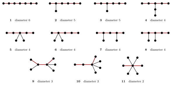
Figure 142: All 11 trees with 7 vertices, numbered as in the table below and grouped by diameter. In each tree the red edges are one longest line in it, and its number of edges is the diameter: 6 for tree 1, 5 for trees 2 and 3, 4 for trees 4 to 8, 3 for trees 9 and 10, and 2 for the star, tree 11. No two of the 11 are the same tree redrawn. Where two share a degree sequence and a diameter, they differ in how the vertices of degree 3 or more sit, as the table explains.
| Tree | Shape | Degree sequence | Diameter | Told apart from the others with the same sequence and diameter by |
|---|---|---|---|---|
| 1 | 7 vertices in a line | \(2, 2, 2, 2, 2, 1, 1\) | 6 | |
| 2 | 6 in a line, one more on the second | \(3, 2, 2, 2, 1, 1, 1\) | 5 | the degree-3 vertex has two neighbours of degree 1 |
| 3 | 6 in a line, one more on the third | \(3, 2, 2, 2, 1, 1, 1\) | 5 | the degree-3 vertex has one neighbour of degree 1 |
| 4 | 5 in a line, a line of two hanging from the middle | \(3, 2, 2, 2, 1, 1, 1\) | 4 | |
| 5 | 5 in a line, two more on the middle | \(4, 2, 2, 1, 1, 1, 1\) | 4 | the degree-4 vertex has two neighbours of degree 1 |
| 6 | 5 in a line, two more on the second | \(4, 2, 2, 1, 1, 1, 1\) | 4 | the degree-4 vertex has three neighbours of degree 1 |
| 7 | 5 in a line, one more on the second and one on the fourth | \(3, 3, 2, 1, 1, 1, 1\) | 4 | the two degree-3 vertices are not joined |
| 8 | 5 in a line, one more on the second and one on the third | \(3, 3, 2, 1, 1, 1, 1\) | 4 | the two degree-3 vertices are joined |
| 9 | two joined vertices, with 2 and 3 more | \(4, 3, 1, 1, 1, 1, 1\) | 3 | |
| 10 | two joined vertices, with 1 and 4 more | \(5, 2, 1, 1, 1, 1, 1\) | 3 | |
| 11 | one vertex joined to the other 6 | \(6, 1, 1, 1, 1, 1, 1\) | 2 |
Renaming vertices keeps degrees and keeps which vertices are joined, so it also keeps facts like “the degree-3 vertex has two neighbours of degree 1”. So in each tied pair the two trees are different, and all 11 are essentially different. Trees 2, 3 and 4 share a degree sequence too, but tree 4 has diameter 4.
Why there are no others. Take two vertices at the largest distance \(d\) in a tree, and a walk of \(d\) edges between them. A shortest walk never repeats a vertex (cutting out the part between two visits would make it shorter), so this walk is a line of \(d + 1\) different vertices, \(v_0, v_1, \dots, v_d\). Every other vertex hangs off this line, and nothing can hang so far out that two vertices end up more than \(d\) apart. A tree with 7 vertices has diameter between 2 and 6: at most 6, since a line of \(d + 1\) different vertices needs \(d + 1 \leq 7\), and at least 2, since diameter 1 would make every two vertices joined, and a tree with 3 or more vertices would then contain a triangle. Going through the diameters:
- \(d = 6\). All 7 vertices are on the line: tree 1.
- \(d = 5\). One vertex is left, joined to \(v_1, v_2, v_3\) or \(v_4\). Joining it to an end would make a longer line. \(v_1\) and \(v_4\) give the same tree by reading the line backwards, and so do \(v_2\) and \(v_3\): trees 2 and 3.
- \(d = 4\). Two vertices are left, \(x\) and \(y\). If both are joined to the line, they hang off \(v_1, v_2\) or \(v_3\), giving the pairs \(\{v_2, v_2\}\), \(\{v_1, v_1\}\), \(\{v_1, v_3\}\) and \(\{v_1, v_2\}\), up to reading backwards: trees 5, 6, 7 and 8. Otherwise \(y\) hangs off \(x\) and \(x\) off the line, and \(x\) must be on the middle vertex \(v_2\), since on \(v_1\) the vertex \(y\) would be 5 from \(v_4\): tree 4.
- \(d = 3\). Three vertices are left, and each must be joined to \(v_1\) or \(v_2\) directly: not to an end, which would make a longer line, and not to another hanging vertex, since a vertex two steps out from \(v_1\) is 4 from \(v_3\), and two steps out from \(v_2\) is 4 from \(v_0\). Splitting 3 as \(0 + 3\) or \(1 + 2\) (up to reading backwards) gives trees 10 and 9.
- \(d = 2\). Every vertex is within 2 of every other: one vertex joined to all six others, tree 11.
That is \(1 + 2 + 5 + 2 + 1 = 11\).
This count, and the next fact, are for interest only and are not assessed. Call a tree homeomorphically irreducible if no vertex has degree 2. There are exactly 10 such trees with 10 vertices. With 7 vertices there are two, trees 9 and 11, the only rows of the table with no 2 in the degree sequence.
Deleting an edge from a tree
Deleting an edge removes that edge and nothing else. Every vertex stays, including the edge’s endpoints.
If any edge is deleted from a tree then the result is a disconnected graph. This disconnected graph consists of two trees.
Figure 143: Deleting the edge \(e\), in red, from the tree \(T\) with 7 vertices and 6 edges. What is left is two trees: \(T_1\), which is \(u\) and the 2 vertices joined to it, and \(T_2\), which is \(v\) and the 3 vertices it can still reach. There is no walk from \(u\) to \(v\) any more, since a shortest such walk together with \(e\) would make a non-trivial circuit in \(T\). The edge counts add up: \(2 + 3 + 1 = 6\).
The proof uses one fact about walks.
Shortcut fact. If there is a walk from \(x\) to \(y\), there is one that visits no vertex twice: take a shortest walk from \(x\) to \(y\). If it visited some vertex twice, cutting out the part between the two visits would leave a shorter walk from \(x\) to \(y\). A walk that visits no vertex twice also uses no edge twice, because the second time it crossed an edge it would arrive at a vertex it had already visited. So it is a trail.
Proof. Let \(T\) be a tree and let \(e\) be an edge of \(T\) with endpoints \(u\) and \(v\). A loop is a non-trivial circuit, so \(e\) is not a loop and \(u \neq v\). Write \(T - e\) for \(T\) with \(e\) deleted.
- There is no walk from \(u\) to \(v\) in \(T - e\). Suppose there were. By the shortcut fact there is one that visits no vertex twice, \(u = w_0\, f_1\, w_1\, f_2 \cdots f_k\, w_k = v\), with \(k \geq 1\) since \(u \neq v\). Its edges \(f_1, \dots, f_k\) are all different, and none of them is \(e\). Then \(u\, f_1\, w_1 \cdots f_k\, v\, e\, u\) ends where it starts and uses no edge twice: a non-trivial circuit in \(T\). That contradicts \(T\) being circuit-free. So \(T - e\) is disconnected.
- Every vertex can reach \(u\) or \(v\) in \(T - e\). Let \(x\) be a vertex. \(T\) is connected, so by the shortcut fact there is a walk from \(x\) to \(u\) in \(T\) that visits no vertex twice. If it does not use \(e\), it is a walk in \(T - e\). If it does, then since \(u\) is an endpoint of \(e\) and the walk meets \(u\) only at the very end, \(e\) is its last edge, crossed from \(v\) to \(u\). Leaving off that last step gives a walk from \(x\) to \(v\) that does not use \(e\).
- Two trees. Let \(T_1\) be the vertices that can reach \(u\) in \(T - e\), and \(T_2\) those that can reach \(v\), each with the edges of \(T - e\) between them. By 2 every vertex is in \(T_1\) or \(T_2\). By 1 no vertex is in both, since a vertex in both would give a walk from \(u\) to \(v\). An edge of \(T - e\) joins two vertices that can reach each other, so both its endpoints are in the same part. So \(T - e\) is exactly \(T_1\) and \(T_2\), with no edge between them. Any two vertices of \(T_1\) can each reach \(u\), so they can reach each other, and every vertex on the way can reach \(u\) too, so the walk stays in \(T_1\). So \(T_1\) is connected, and likewise \(T_2\). A non-trivial circuit in \(T_1\) or \(T_2\) would be one in \(T\), so both are circuit-free. So \(T_1\) and \(T_2\) are trees. \(\square\)
Two things to take into the next section: \(T_1\) contains \(u\) and \(T_2\) contains \(v\), so each has at least one vertex; and every edge of \(T\) except \(e\) is in exactly one of \(T_1\) and \(T_2\).
A tree with \(n\) vertices has \(n - 1\) edges
Theorem. A graph \(G\) with \(n\) vertices is a tree if and only if it is simple, connected and has \(n - 1\) edges.
There are two directions to prove.
(\(\Rightarrow\)) Every tree is simple, connected and has \(n - 1\) edges
A tree is connected by definition, and it is simple because it is circuit-free (above). What is left is the edge count, by strong induction on \(n\).
Let \(P(n)\) be: every tree with \(n\) vertices has \(n - 1\) edges.
Basis, \(n = 1\). A tree with one vertex has no edges: an edge would have to be a loop at that vertex, and a loop is a non-trivial circuit. \(0 = 1 - 1\), so \(P(1)\) holds.
Inductive hypothesis. Let \(k \geq 1\) be an integer, and suppose that every tree with \(p\) vertices, for every \(p\) with \(1 \leq p \leq k\), has \(p - 1\) edges.
Inductive step. Let \(T\) be a tree with \(k + 1\) vertices. Since \(k + 1 \geq 2\), \(T\) has two different vertices, and as \(T\) is connected there is a walk between them. That walk uses an edge, so \(T\) has an edge \(e\). Delete it. By the previous section this leaves two trees, \(T_1\) with \(p\) vertices and \(T_2\) with \(q\) vertices, where \(p, q \geq 1\) and \(p + q = k + 1\). So \(p \leq k\) and \(q \leq k\), and by the inductive hypothesis \(T_1\) has \(p - 1\) edges and \(T_2\) has \(q - 1\). Every edge of \(T\) is \(e\) or is in exactly one of \(T_1\), \(T_2\), so \(T\) has
\[(p - 1) + (q - 1) + 1 = p + q - 1 = (k + 1) - 1 = k\]
edges. So \(P(k + 1)\) holds, and by strong induction \(P(n)\) holds for every integer \(n \geq 1\). \(\square\)
The induction has to be strong because \(p\) and \(q\) can be any sizes from 1 to \(k\), not just \(k\) (strong-induction-and-the-well-ordering-principle).
Figure 144: The inductive step on a tree with 13 vertices. Deleting the red edge \(e\) leaves two trees: \(T_1\) with \(p = 6\) vertices and \(T_2\) with \(q = 7\). Both are smaller than the whole tree, so the inductive hypothesis gives them \(p - 1 = 5\) and \(q - 1 = 6\) edges. Putting \(e\) back gives \(5 + 6 + 1 = 12 = 13 - 1\) edges, which is \((p - 1) + (q - 1) + 1 = p + q - 1\).
(\(\Leftarrow\)) A simple connected graph with \(n - 1\) edges is a tree
This direction is by contradiction, and it needs one more fact.
Lemma. If \(G\) is connected and \(e\) is an edge of a non-trivial circuit in \(G\), then \(G - e\) is still connected.
Proof. Write the circuit as \(v_0\, e_1\, v_1 \cdots e_m\, v_m\) with \(v_0 = v_m\), and say \(e = e_i\), with endpoints \(v_{i-1}\) and \(v_i\). The edges of a circuit are all different, so \(e\) appears in it only once. Going the other way round the circuit,
\[R:\quad v_i\, e_{i+1}\, v_{i+1} \cdots e_m\, v_m = v_0\, e_1\, v_1 \cdots e_{i-1}\, v_{i-1}\]
is a walk from \(v_i\) to \(v_{i-1}\) that uses every edge of the circuit except \(e\). Now let \(x\) and \(y\) be any two vertices. \(G\) is connected, so there is a walk from \(x\) to \(y\) in \(G\). Each time it crosses \(e\) it steps from \(v_{i-1}\) to \(v_i\) or from \(v_i\) to \(v_{i-1}\); replace that step by \(R\) backwards or by \(R\). The result is a walk from \(x\) to \(y\) that does not use \(e\). So \(G - e\) is connected. \(\square\)
(If \(e\) is a loop then \(v_{i-1} = v_i\) and \(R\) is a walk from that vertex back to itself; the same replacement works.)
Figure 145: Deleting an edge of a circuit keeps a graph connected. Left: a connected graph whose four middle vertices form a circuit, and the walk from \(x\) to \(y\) through the edge \(e\). Right: \(e\) is deleted, and the walk goes round the rest of the circuit instead, in red. The left graph has 6 vertices and 6 edges, one more than a tree with 6 vertices. The right graph is connected with no circuit, a tree with \(6 - 1 = 5\) edges.
Proof of (\(\Leftarrow\)). Let \(G\) be a simple connected graph with \(n\) vertices and \(n - 1\) edges, and suppose, for a contradiction, that \(G\) is not a tree. \(G\) is connected, so it is not circuit-free: it has a non-trivial circuit. Delete one edge of that circuit. By the lemma the graph is still connected, and it still has all \(n\) vertices. If it still has a non-trivial circuit, delete an edge of that one, and keep going. Each deletion removes an edge and keeps the graph connected, and \(G\) has only finitely many edges, so this stops, at a graph \(H\) with no non-trivial circuit. \(H\) is connected and circuit-free, so it is a tree with \(n\) vertices. At least one edge was deleted, so \(H\) has at most \(n - 2\) edges. But by (\(\Rightarrow\)), a tree with \(n\) vertices has exactly \(n - 1\) edges. This is a contradiction, so \(G\) is a tree. \(\square\)
Two remarks on the proof.
- The word simple is never used in (\(\Leftarrow\)). A connected graph with \(n\) vertices and \(n - 1\) edges is already a tree, and so it turns out to be simple.
- Neither direction uses anything about vertices of degree 1. So the next worked question, which proves a fact about them from this theorem, is not going round in a circle.
Worked: degree 3 or degree 1
Every vertex of a tree with 15 edges has either degree 3 or degree 1. How many vertices of the tree have degree 3?
Answer: 7.
A tree with 15 edges has \(15 + 1 = 16\) vertices, by the theorem. Let \(x\) be the number of vertices of degree 3. Then \(16 - x\) vertices have degree 1.
By the Handshake Theorem (graphs) the degrees add to \(2 \cdot 15 = 30\). The degree sum is \(3 + 3 + \cdots + 3\), \(x\) times, plus \(1 + 1 + \cdots + 1\), \(16 - x\) times:
\[3x + (16 - x) = 30, \qquad 2x = 14, \qquad x = 7.\]
So 7 vertices have degree 3 and 9 have degree 1. Check: \(7 \cdot 3 + 9 \cdot 1 = 30 = 2 \cdot 15\).
The count shows what any such tree must have. One such tree:
Figure 146: A tree with 15 edges in which every vertex has degree 3 or 1. The 7 vertices of degree 3, in red, lie in a line. The two at the ends each have two more vertices of degree 1 joined to them, and the five in between have one each, so there are \(2 + 5 + 2 = 9\) vertices of degree 1. That is 16 vertices and \(6 + 9 = 15\) edges, and the degrees add to \(7 \cdot 3 + 9 \cdot 1 = 30\).
Worked: how many vertices
A tree has two vertices of degree 4, one vertex of degree 2, and all the other vertices have degree 1. How many vertices does the tree have?
Answer: 9.
Three vertices have degree 4 or 2. Let \(x\) be the number of vertices of degree 1, and \(n\) the total number of vertices, so
\[n = x + 3.\]
By the theorem the tree has \(n - 1 = (x + 3) - 1 = x + 2\) edges. By the Handshake Theorem the degrees add to \(2(x + 2)\):
\[2 \cdot 4 + 1 \cdot 2 + x = 2(x + 2), \qquad 10 + x = 2x + 4, \qquad x = 6.\]
So \(n = x + 3 = 9\). Check: the degrees add to \(4 + 4 + 2 + 6 \cdot 1 = 16 = 2 \cdot 8\), and \(8 = 9 - 1\) edges.
Figure 147: A tree with two vertices of degree 4, one of degree 2 and the rest of degree 1. The vertex of degree 2 sits between the two of degree 4, and each of those has three more vertices of degree 1 joined to it. That is \(3 + 6 = 9\) vertices and 8 edges, and the degrees add to \(4 + 4 + 2 + 6 = 16 = 2 \cdot 8\).
Both questions use the same two facts: a tree with \(n\) vertices has \(n - 1\) edges, and the degrees add to twice the number of edges. Naming the unknown count and writing both facts down gives an equation to solve. The method is in trees.
Worked: two vertices of degree 1
Prove that every tree with at least two vertices has at least two vertices of degree 1.
Proof (by contradiction). Suppose there is a tree \(T\) with \(n \geq 2\) vertices that has at most one vertex of degree 1.
By the theorem \(T\) has \(n - 1\) edges, so by the Handshake Theorem
\[\sum_{v \in V(T)} \deg(v) = 2(n - 1) = 2n - 2.\]
Since \(T\) is a tree it is connected, and since it has at least 2 vertices, every vertex has a walk to some other vertex, so no vertex has degree 0. There are two cases.
- No vertex of degree 1. Then every vertex has degree at least 2, and \(\sum \deg(v) \geq 2n\).
- Exactly one vertex of degree 1. All the others have degree at least 2, and \(\sum \deg(v) \geq 1 + 2(n - 1) = 2n - 1\).
In either case \(\sum \deg(v) \geq 2n - 1\). But the sum is \(2n - 2\), so \(2n - 2 \geq 2n - 1\), that is \(-2 \geq -1\), which is false. So every tree with at least two vertices has at least two vertices of degree 1. \(\square\)
Both conditions matter. A line of vertices has exactly two vertices of degree 1, its ends, so “two” cannot be improved. And the tree with one vertex has no vertex of degree 1 at all: its only vertex has degree 0. More on vertices of degree 1, including a second proof, is in trees.
Worked: degrees \(n - 2\) and \(n - 3\)
Prove that if there exists a tree with \(n\) vertices that has a vertex of degree \(n - 2\) and another vertex of degree \(n - 3\), then \(n \leq 5\).
Read it as: if any tree with \(n\) vertices has these two degrees, then \(n \leq 5\). The two vertices have different degrees, so they are automatically two different vertices.
Proof (by contradiction). Let \(T\) be a tree with \(n \geq 6\) vertices that has a vertex \(v_1\) of degree \(n - 2\) and a vertex \(v_2\) of degree \(n - 3\).
By the theorem \(T\) has \(n - 1\) edges, so by the Handshake Theorem
\[\sum \deg(v) = 2(n - 1) = 2n - 2.\]
Since \(T\) is connected and has at least 2 vertices, no vertex has degree 0, so every vertex has degree at least 1. Apart from \(v_1\) and \(v_2\) there are \(n - 2\) vertices, and \(n - 2 \geq 4\) since \(n \geq 6\). They contribute at least 1 each, so at least 4 in all:
\[\sum \deg(v) \geq (n - 3) + (n - 2) + 4 = 2n - 5 + 4 = 2n - 1.\]
So \(2n - 2 \geq 2n - 1\), which is false. So \(n \leq 5\). \(\square\)
The same count without contradiction: if such a tree exists then \(n - 3 \geq 0\), so \(n \geq 3\) and every degree is at least 1. Then
\[2n - 2 = \sum \deg(v) \geq (n - 2) + (n - 3) + (n - 2) = 3n - 7,\]
which gives \(n \leq 5\).
The bound is reached. With \(n = 5\), a vertex of degree 3 and a vertex of degree 2: join \(v_1\) to \(v_2\) and to two more vertices, and \(v_2\) to a fifth. With \(n = 4\), a vertex of degree 2 and another of degree 1: four vertices in a line. With \(n = 3\) the second vertex would need degree 0, which no tree with at least two vertices has, and with \(n \leq 2\) the degree \(n - 3\) is negative. So the trees with this property have exactly 4 or 5 vertices.
Figure 148: Trees with a vertex of degree \(n - 2\) and another of degree \(n - 3\), the two in red. Left, \(n = 5\): degrees 3 and 2, and the other three vertices have degree 1. The degrees add to \(3 + 2 + 1 + 1 + 1 = 8 = 2 \cdot 4\). Right, \(n = 4\): four vertices in a line, with degrees 2 and 1 marked. With \(n = 6\) the two red vertices alone would need degrees \(4 + 3 = 7\), the four others at least 4 more, and \(11\) is more than the \(2 \cdot 5 = 10\) a tree with 6 vertices allows.
See also
- [trees] — trees, the \(n - 1\) theorem, vertices of degree 1, and the counting method
- walks-trails-and-circuits — walks, trails, circuits and connected graphs
- graphs — the degrees add to twice the number of edges
- strong-induction-and-the-well-ordering-principle — the induction used for (\(\Rightarrow\))
- proof-techniques — the method used for (\(\Leftarrow\)) and Worked questions 3 and 4
- 2026-10-27-matrix-representations-of-graphs — Lecture 35
- practice-problems — §46, with full worked solutions
Reference material
Adjacency Matrices
An adjacency matrix writes a graph down as a square table of numbers: a row and a column for each vertex, and in each place the number of edges joining that pair of vertices. It records everything about the graph except the names of the edges, so the graph can be redrawn from it, and the degrees, and with them whether the graph has an Euler circuit, can be read straight off it. The one trap is the loop, which counts 1 in the matrix but 2 in the degree. The other matrix of a graph, with a row for each vertex and a column for each edge, is in incidence-matrices. Graphs, loops, degree and the Handshake Theorem are in [graphs]. First met in 2026-10-27-matrix-representations-of-graphs.
Definition
The adjacency matrix of a graph with vertices \(v_1, v_2, \dots, v_n\) is the \(n \times n\) matrix \(A = [a_{ij}]\) where each entry \(a_{ij}\) is the number of edges with endpoints \(\{v_i, v_j\}\).
Figure 149: A graph and its adjacency matrix. Each entry counts the edges joining the vertex of its row to the vertex of its column: the 2 in row v2, column v3 is the two parallel edges e1 and e2, and the 0 in row v1, column v3 says v1 and v3 are not adjacent. The diagonal counts loops, so the single loop e5 gives a 1 in row v4, column v4. Every entry appears again reflected in the diagonal, because the edges between v2 and v3 are the edges between v3 and v2.
What the definition gives straight away:
- \(A\) is square, \(n \times n\), with one row and one column for each vertex.
- Every entry is a non-negative integer, since it counts edges.
- \(A\) is symmetric: \(a_{ij} = a_{ji}\) for all \(i, j\). The set \(\{v_i, v_j\}\) is the same set as \(\{v_j, v_i\}\), so the two entries count the same edges. Everything below the diagonal repeats something above it.
- Off the diagonal, \(a_{ij} \ge 1\) exactly when \(v_i\) and \(v_j\) are adjacent, and \(a_{ij} \ge 2\) exactly when they are joined by parallel edges.
- On the diagonal, \(a_{ii}\) is the number of loops at \(v_i\). See loops.
- An isolated vertex has a row and a column of zeros. It still gets its row, because the matrix has one for every vertex.
Simple graphs. A graph is simple when it has no loops and no parallel edges (graphs). In the matrix that is: every entry is 0 or 1, and the diagonal is all 0. The complete graph \(K_4\), for example, has a 1 in every place off the diagonal:
\[\begin{array}{c|cccc} & v_1 & v_2 & v_3 & v_4 \\ \hline v_1 & 0 & 1 & 1 & 1 \\ v_2 & 1 & 0 & 1 & 1 \\ v_3 & 1 & 1 & 0 & 1 \\ v_4 & 1 & 1 & 1 & 0 \end{array}\]
The matrix depends on the order of the vertices. Listing the same vertices in a different order rearranges the rows and the columns in the same way. With the vertices of the graph above in the order \(v_2, v_3, v_1, v_4\), the matrix is
\[\begin{array}{c|cccc} & v_2 & v_3 & v_1 & v_4 \\ \hline v_2 & 0 & 2 & 1 & 0 \\ v_3 & 2 & 0 & 0 & 0 \\ v_1 & 1 & 0 & 0 & 1 \\ v_4 & 0 & 0 & 1 & 1 \end{array}\]
a different matrix for the same graph. So a graph has an adjacency matrix for each order of its vertices, and the rows and columns should always be labelled.
The matrix does not name the edges. It says there are two edges between \(v_2\) and \(v_3\), but not which is \(e_1\). A graph rebuilt from its adjacency matrix is the same graph up to the names of the edges.
Loops
A loop at \(v_i\) is one edge whose set of endpoints is \(\{v_i\} = \{v_i, v_i\}\), so it adds 1 to the diagonal entry \(a_{ii}\). In the graph above the one loop \(e_5\) gives \(a_{44} = 1\). Two loops at a vertex give a 2 on the diagonal, and the \(1 \times 1\) matrix \([73]\) is a single vertex with 73 loops.
A loop adds 2 to the degree of its vertex (graphs) but only 1 to the matrix. So when there are loops, the row sum is not the degree.
Degree from the adjacency matrix. For each vertex \(v_i\), \[\deg(v_i) = (a_{i1} + a_{i2} + \cdots + a_{in}) + a_{ii},\] the sum of row \(i\) plus the diagonal entry of row \(i\).
Proof. Every edge with \(v_i\) as an endpoint is counted exactly once in row \(i\): an edge joining \(v_i\) to a different vertex \(v_j\) in \(a_{ij}\), and a loop at \(v_i\) in \(a_{ii}\). An edge joining \(v_i\) to a different vertex has one end at \(v_i\) and adds 1 to \(\deg(v_i)\), the same as it adds to the row. A loop has both of its ends at \(v_i\) and adds 2 to \(\deg(v_i)\), one more than it adds to the row. So the degree is the row sum plus one for each loop at \(v_i\), and there are \(a_{ii}\) loops at \(v_i\). \(\square\)
In the graph above:
| Vertex | Row sum | Diagonal entry | Degree |
|---|---|---|---|
| \(v_1\) | \(0 + 1 + 0 + 1 = 2\) | 0 | 2 |
| \(v_2\) | \(1 + 0 + 2 + 0 = 3\) | 0 | 3 |
| \(v_3\) | \(0 + 2 + 0 + 0 = 2\) | 0 | 2 |
| \(v_4\) | \(1 + 0 + 0 + 1 = 2\) | 1 | 3 |
\(v_4\) meets \(e_4\) once and the loop \(e_5\) twice, so its degree is 3, not the row sum 2. For a graph without loops the diagonal is all 0 and the degree is just the row sum.
Counting the edges. Each edge is counted exactly once on or above the diagonal: an edge joining \(v_i\) and \(v_j\) with \(i < j\) in \(a_{ij}\), and a loop on the diagonal. So
\[\text{number of edges} = \sum_{i \le j} a_{ij},\]
the sum of the diagonal and everything above it. Above, that is \((0 + 1 + 0 + 1) + (0 + 2 + 0) + (0 + 0) + 1 = 5\). Adding up every entry counts each non-loop edge twice, once on each side of the diagonal, and each loop once, so adding the diagonal on top gives \(2e\). That is the degree formula summed over all the vertices, and it is the Handshake Theorem (graphs): above, \(9 + 1 = 10 = 2 \cdot 5\).
Reading a graph off a matrix
Given an adjacency matrix, the graph is drawn from the diagonal and the entries above it:
- Check it is an adjacency matrix: square, symmetric, non-negative integer entries (below).
- Draw a dot for each row and label it \(v_1, \dots, v_n\) in order.
- For each \(i < j\), draw \(a_{ij}\) edges between \(v_i\) and \(v_j\).
- For each \(i\), draw \(a_{ii}\) loops at \(v_i\).
- Ignore everything below the diagonal. It repeats what is above, and reading it too would draw every edge twice.
Then check: the number of edges drawn is the sum on and above the diagonal, and each degree in the drawing is its row sum plus its diagonal entry.
For example, take
\[M = \begin{array}{c|cccc} & v_1 & v_2 & v_3 & v_4 \\ \hline v_1 & 1 & 1 & 0 & 0 \\ v_2 & 1 & 0 & 2 & 1 \\ v_3 & 0 & 2 & 0 & 1 \\ v_4 & 0 & 1 & 1 & 0 \end{array}\]
It is square, symmetric and has non-negative integer entries. On and above the diagonal: \(a_{11} = 1\) is a loop at \(v_1\); \(a_{12} = 1\) is an edge \(v_1 v_2\); \(a_{23} = 2\) is two parallel edges \(v_2 v_3\); \(a_{24} = 1\) and \(a_{34} = 1\) are edges \(v_2 v_4\) and \(v_3 v_4\). Every other entry there is 0. That is 6 edges.
Figure 150: Reading a graph off an adjacency matrix. Only the diagonal and the entries above it, in blue, are used: each entry above the diagonal is a number of edges between two vertices, and each diagonal entry is a number of loops. The grey entries below the diagonal repeat the blue ones and are skipped. The blue entries add to 6, the number of edges. The degrees, in red, are row sum plus diagonal entry: v1 has row sum 2 and one loop, so degree 3.
The degrees are \(\deg(v_1) = 2 + 1 = 3\), \(\deg(v_2) = 4\), \(\deg(v_3) = 3\) and \(\deg(v_4) = 2\), adding to \(12 = 2 \cdot 6\). A larger example, with two loops and three parallel edges, is worked in 2026-10-27-matrix-representations-of-graphs.
Which matrices are adjacency matrices
A matrix is the adjacency matrix of some graph if and only if it is square (with at least one row), symmetric, and every entry is a non-negative integer \(0, 1, 2, \dots\)
Proof. (\(\Rightarrow\)) Shown under the definition: an adjacency matrix has a row and a column for each vertex, a graph has at least one vertex, every entry counts edges, and \(\{v_i, v_j\} = \{v_j, v_i\}\).
(\(\Leftarrow\)) Let \(M = [m_{ij}]\) be an \(n \times n\) symmetric matrix with \(n \ge 1\) and non-negative integer entries. Build a graph with vertices \(v_1, \dots, v_n\): for each \(i < j\) put \(m_{ij}\) edges between \(v_i\) and \(v_j\), and for each \(i\) put \(m_{ii}\) loops at \(v_i\). These are whole numbers of edges, at least 0, so this is a graph. The number of edges with endpoints \(\{v_i, v_j\}\) is then \(m_{ij}\) when \(i < j\), it is \(m_{ii}\) when \(i = j\), and when \(i > j\) it is \(m_{ji}\), which equals \(m_{ij}\) because \(M\) is symmetric. So \(M\) is this graph’s adjacency matrix. \(\square\)
So there are three things to check, and a matrix fails if any one of them fails:
| Matrix | Square | Symmetric | Entries in \(0, 1, 2, \dots\) | Adjacency matrix? |
|---|---|---|---|---|
| \(\begin{bmatrix} 0 & 2 \\ 2 & 1 \end{bmatrix}\) | yes | yes | yes | yes: two parallel edges and a loop at \(v_2\) |
| \(\begin{bmatrix} 0 & 1 & 1 \end{bmatrix}\) | no | — | yes | no: one row, three columns |
| \(\begin{bmatrix} 0 & 1 \\ 0 & 0 \end{bmatrix}\) | yes | no | yes | no |
| \(\begin{bmatrix} 0 & \tfrac12 \\ \tfrac12 & 0 \end{bmatrix}\) | yes | yes | no | no: half an edge |
| \(\begin{bmatrix} 0 & 0 \\ 0 & 0 \end{bmatrix}\) | yes | yes | yes | yes: two isolated vertices, no edges |
Nothing else is needed. The diagonal can hold any non-negative integer, and so can any entry off it. Four more are worked in 2026-10-27-matrix-representations-of-graphs.
Degrees and Euler circuits
The matrix holds everything needed to decide whether a graph has an Euler circuit (euler-circuits-and-trails): a connected graph has one exactly when every vertex has even degree.
- The degrees are row sum plus diagonal entry, as above.
- Connectedness can be read off too. The graph is not connected exactly when the vertices split into two non-empty groups with a 0 in every entry between a vertex of one group and a vertex of the other: then no edge crosses between the groups.
For \(M\) above the degrees are \(3, 4, 3, 2\). The graph is connected, since \(v_2\) is joined to every other vertex. Two vertices, \(v_1\) and \(v_3\), have odd degree, so there is no Euler circuit, but there is an Euler trail from \(v_1\) to \(v_3\). For the graph in the definition the odd vertices are \(v_2\) and \(v_4\), so it too has an Euler trail and no Euler circuit.
A degree must be computed with the diagonal added in before its parity is judged. A vertex with row sum 2 and one loop has degree 3, which is odd.
Common mistakes
- Writing 2 on the diagonal for a loop. The adjacency matrix counts edges, and a loop is one edge, so it counts 1. The 2 for a loop belongs in the incidence matrix, which counts how many times a vertex meets an edge.
- Taking the row sum as the degree when there are loops. Add the diagonal entry: \(\deg(v_i)\) is the row sum plus \(a_{ii}\).
- Reading the whole matrix when drawing. Every entry off the diagonal appears twice. Read the diagonal and above only, or every edge comes out doubled.
- Counting edges by adding all the entries. That counts each non-loop edge twice. Add the diagonal and the entries above it.
- Expecting a zero diagonal and only 0s and 1s. That is true for simple graphs only. Loops put numbers on the diagonal, and parallel edges put numbers bigger than 1 off it.
- Leaving off the labels. The matrix depends on the order of the vertices, so label the rows and columns.
- Accepting a matrix that is not symmetric. \(a_{ij}\) and \(a_{ji}\) count the same edges and must be equal.
See also
- incidence-matrices — the other matrix of a graph, with a column for each edge, and how the two compare
- [graphs] — loops, parallel edges, simple graphs, degree and the Handshake Theorem
- euler-circuits-and-trails — the even-degree test for an Euler circuit
- walks-trails-and-circuits — connected graphs
- 2026-10-27-matrix-representations-of-graphs — Lecture 35
- practice-problems — §45, with full worked solutions
Antisymmetric Relations
A relation is antisymmetric when no two different elements are related in both directions. It is the property that takes the place of symmetry in a partial order (partial-order-relations). In spite of the name it is not the opposite of symmetric. The other three properties are in reflexive-symmetric-and-transitive-relations. First met in 2026-09-22-partial-order-relations.
The definition
A relation \(R\) on a set \(S\) is antisymmetric if and only if \[\forall a, b \in S,\ (a \mathrel{R} b \text{ and } b \mathrel{R} a) \to (a = b).\]
There are two equivalent definitions:
\[\forall a, b \in S,\ (a \neq b) \to {\sim}(a \mathrel{R} b \text{ and } b \mathrel{R} a).\] \[\forall a, b \in S,\ (a \mathrel{R} b \text{ and } a \neq b) \to {\sim}(b \mathrel{R} a).\]
The first is the easiest for proving a relation antisymmetric, and the third is the most intuitive.
| In words | |
|---|---|
| first | If \(a\) and \(b\) are related both ways, they are the same element. |
| second | Two different elements are not related both ways. |
| third | If \(a\) is related to a different element \(b\), then \(b\) is not related back to \(a\). |
Why the three say the same thing
Write \(p\) for \(a \mathrel{R} b\), \(q\) for \(b \mathrel{R} a\) and \(r\) for \(a = b\). The three definitions are the conditionals
\[(p \land q) \to r, \qquad {\sim}r \to {\sim}(p \land q), \qquad (p \land {\sim}r) \to {\sim}q.\]
The second is the contrapositive of the first (conditional-statements). For the third, recall that a conditional is false in only one situation, a true hypothesis with a false conclusion. Work out that situation for each:
| Conditional | False exactly when |
|---|---|
| \((p \land q) \to r\) | \(p\) true, \(q\) true, \(r\) false |
| \({\sim}r \to {\sim}(p \land q)\) | \(r\) false, \(p\) true, \(q\) true |
| \((p \land {\sim}r) \to {\sim}q\) | \(p\) true, \(r\) false, \(q\) true |
It is the same situation each time, so the three are logically equivalent. Each one forbids exactly one thing: \(a \mathrel{R} b\) and \(b \mathrel{R} a\) with \(a \neq b\).
In the arrow diagram
Antisymmetric: no two different dots are joined by arrows both ways. Loops are not restricted. When \(a = b\) the first definition reads \((a \mathrel{R} a \text{ and } a \mathrel{R} a) \to (a = a)\), which is true whether or not there is a loop at \(a\).
Between two different elements there are three possibilities, and symmetry and antisymmetry each rule out a different one.
Figure 151: What symmetry and antisymmetry allow between two different elements. With no arrow, both are satisfied. A single arrow has no return, which breaks symmetry and is fine for antisymmetry. Arrows both ways are what symmetry asks for, and they break antisymmetry. So a symmetric relation has no single arrows, and an antisymmetric relation has no two-way pairs. A loop joins an element to itself and breaks neither.
Antisymmetric is not “not symmetric”
Antisymmetric \(\neq\) not symmetric. The two properties are independent, and all four combinations occur. The diagrams are the four of 2026-09-22-partial-order-relations.
| antisymmetric | not antisymmetric | |
|---|---|---|
| symmetric | Diagram 2. Only loops. Also: \(=\) on any set. | Diagram 3. Two-way pairs, no single arrows. Also: same parity on \(\mathbb{Z}\). |
| not symmetric | Diagram 4. Single arrows, no two-way pairs. Also: \(\leq\) on \(\mathbb{R}\), \(\subseteq\), divides on \(\mathbb{Z}^{+}\). | Diagram 1. A single arrow and a two-way pair. |
The definitions make the difference exact:
- not symmetric says there is an arrow with no return;
- antisymmetric says no arrow between different elements has a return.
A relation that is not symmetric can still have some two-way pairs, as Diagram 1 does, and then it is not antisymmetric either.
Both at once. If \(R\) is symmetric and antisymmetric, every arrow is a loop. Suppose \(a \mathrel{R} b\). Symmetry gives \(b \mathrel{R} a\), and then antisymmetry gives \(a = b\). So the only relations with both properties are those in which no element is related to anything but itself, like Diagram 2.
Proving and disproving
Antisymmetry is a “for all”, so it is proved with arbitrary elements and disproved with one witness.
| How | |
|---|---|
| To prove it | Let \(a, b \in S\) and suppose \(a \mathrel{R} b\) and \(b \mathrel{R} a\). Unfold both. Show \(a = b\). |
| To disprove it | Find two different elements \(a, b\) with \(a \mathrel{R} b\) and \(b \mathrel{R} a\). |
In the proof, write the goal down before starting: (Goal: show \(a = b\)). Both hypotheses will be needed.
Worked: divides on \(\mathbb{Z}^{+}\)
Worked in full in 2026-09-22-partial-order-relations. Let \(a, b \in \mathbb{Z}^{+}\) and suppose \(a \mid b\) and \(b \mid a\). (Goal: show \(a = b\).) Then \(b = ak\) and \(a = b\ell\) for some \(k, \ell \in \mathbb{Z}\). Substituting, \[b = ak = (b\ell)k = b(\ell k),\] and since \(b \neq 0\), \(\ell k = 1\). Now \(a, b > 0\) forces \(k > 0\) and \(\ell > 0\), and the only positive integers with product 1 are \(\ell = k = 1\). So \(a = b\).
The last step uses that the set is \(\mathbb{Z}^{+}\). See Examples for what goes wrong on \(\mathbb{Z}\).
Worked: a disproof
From practice-problems, Q2. On binary strings of length 6, let \(s \mathrel{\rho} t\) if and only if \(\operatorname{weight}(s) \leq \operatorname{weight}(t)\), where the weight is the number of ones. Take \(s = 100000\) and \(t = 010000\). Both have weight 1, so \(s \mathrel{\rho} t\) and \(t \mathrel{\rho} s\), but \(s \neq t\). So \(\rho\) is not antisymmetric.
Two different things with the same weight are related both ways. Any relation that compares elements through a number they can share fails in the same way.
The third form in a proof
The first definition is the easiest to prove from, but the third works too. The solution to practice-problems, Q1 uses it: suppose \(x \mathrel{\rho} y\) where \(x \neq y\); we must show that then \(y \mathrel{\not\rho} x\). Either is acceptable. State which you are using.
Examples
The standard examples, with reasons:
| Relation | on | Antisymmetric because |
|---|---|---|
| \(\leq\) | \(\mathbb{R}\) | \((x \leq y \text{ and } y \leq x) \to x = y\) |
| \(\geq\) | \(\mathbb{R}\) | the same, reversed |
| \(<\), \(>\) | \(\mathbb{R}\) | \(x < y\) and \(y < x\) never hold together |
| divides | \(\mathbb{Z}^{+}\) | proved above |
| \(\subseteq\) | any set \(S\) of sets | \((X \subseteq Y \text{ and } Y \subseteq X) \to X = Y\) |
\(<\) is antisymmetric vacuously. For no \(x, y\) are \(x < y\) and \(y < x\) both true. The hypothesis of the first definition is therefore always false, and a conditional with a false hypothesis is true (conditional-statements). In the diagram of \(<\) there are no two-way pairs, and no loops either.
\(\subseteq\) is the double-containment rule. Showing \(X \subseteq Y\) and \(Y \subseteq X\) to conclude \(X = Y\) is how set equality is proved (sets-and-set-notation). Antisymmetry of \(\subseteq\) is that rule under another name.
Divides is not antisymmetric on \(\mathbb{Z}\). \(2 \mid -2\), since \(-2 = 2 \cdot (-1)\), and \(-2 \mid 2\), since \(2 = (-2)(-1)\), but \(2 \neq -2\). This is why the statement is about \(\mathbb{Z}^{+}\). A relation is always a relation on a particular set, and the same rule on a bigger set can lose a property.
Not antisymmetric: any relation with two different elements related both ways. That includes congruence mod \(n\) for \(n \geq 1\), same parity, and every equivalence relation that has a class with more than one element.
Common mistakes
- Reading “antisymmetric” as “not symmetric”. See the four combinations above.
- Thinking a loop breaks antisymmetry. It does not. The property is about pairs of different elements.
- Proving it from an example. “\(2 \mid 4\) but \(4 \nmid 2\)” shows one pair behaves. Antisymmetry is about all pairs.
- Using only one hypothesis. A proof that starts “suppose \(a \mathrel{R} b\)” and never uses \(b \mathrel{R} a\) cannot reach \(a = b\).
- Disproving with \(a = b\). A witness needs two different elements. \(a \mathrel{R} a\) on its own shows nothing.
See also
- partial-order-relations — reflexive, antisymmetric and transitive together
- reflexive-symmetric-and-transitive-relations — the other three properties, and how to prove and disprove them
- conditional-statements — the contrapositive, and vacuous truth
- divisibility-and-factorisation — the definition of divides
- 2026-09-22-partial-order-relations — Lecture 25
- practice-problems — §32, with full worked solutions
Binomial Coefficients
The numbers \(\binom{n}{r}\) count subsets, and they are also the coefficients that appear when \((a + b)^n\) is multiplied out, which is where the name binomial coefficient comes from. This note collects the identities they satisfy and the way each is proved by counting: the symmetry \(\binom{n}{r} = \binom{n}{n-r}\), Pascal’s formula and the triangle it builds, the Binomial Theorem, how to pick a single coefficient out of an expansion such as \((3x - 2)^5\), and why every row of Pascal’s triangle adds up to a power of 2. The definition and the formula \(\frac{n!}{r!\,(n-r)!}\) are in counting-selections. Using these counts to work out probabilities is in [probability]. First met in 2026-10-19-probability-binomial-coefficients.
\(n\) choose \(r\)
\(\binom{n}{r}\), read “\(n\) choose \(r\)”, is the number of \(r\)-element subsets of a set with \(n\) elements:
\[\binom{n}{r} = \frac{n!}{r!\,(n-r)!} = \frac{n(n-1)\cdots(n-r+1)}{r(r-1)\cdots 1}, \qquad 0 \le r \le n.\]
Why it divides by \(r!\), and how to calculate it without large factorials, is in counting-selections. Two values come up constantly: \(\binom{n}{0} = \binom{n}{n} = 1\) (one way to take nothing, one way to take everything) and \(\binom{n}{1} = n\).
Everything below rests on reading \(\binom{n}{r}\) as a count, not as a formula. Most identities about binomial coefficients can be proved by grinding through factorials, but each one is also the statement that two ways of counting the same collection agree, and that version explains why it is true.
Combinatorial proofs
A combinatorial proof of an identity \(\text{LHS} = \text{RHS}\) finds one collection of objects and counts it twice: once in a way that gives the left side, once in a way that gives the right side. Both counts are counts of the same thing, so they are equal. No algebra is needed. The work is in choosing the collection, and in checking that each count really counts every object exactly once.
There are two common shapes.
- A pairing. Match the objects counted by the left side one-to-one with the objects counted by the right side. That is how the symmetry is proved: each subset is paired with its complement.
- Splitting into cases. Count a collection directly for one side, and split it into disjoint cases, added up, for the other. That is how Pascal’s formula and the row sum are proved.
Symmetry: \(\binom{n}{r} = \binom{n}{n-r}\)
For \(0 \le r \le n\), \[\binom{n}{r} = \binom{n}{n-r}.\]
Why. Choosing which \(r\) elements of an \(n\)-element set go into a subset is the same act as choosing which \(n - r\) elements are left out. Every \(r\)-element subset \(A\) has a complement, the \(n - r\) elements not in \(A\), and every \((n - r)\)-element subset is the complement of exactly one \(r\)-element subset. So the subsets of the two sizes pair off exactly, and there are the same number of each.
Figure 152: The ten 2-element subsets of \({1, 2, 3, 4, 5}\), each joined to its complement, the three elements it leaves out. Every 2-element subset has exactly one complement, and every 3-element subset is the complement of exactly one 2-element subset, so the two lists pair off with nothing left over. That pairing is the proof that \(\binom52 = \binom53 = 10\), and the same pairing of each \(r\)-element subset with its complement proves \(\binom{n}{r} = \binom{n}{n-r}\).
Using it. Calculate whichever of the two has the smaller bottom number:
\[\binom{12}{8} = \binom{12}{4} = \frac{12 \cdot 11 \cdot 10 \cdot 9}{4 \cdot 3 \cdot 2 \cdot 1} = 495, \qquad \binom{7}{4} = \binom{7}{3} = \frac{7 \cdot 6 \cdot 5}{3 \cdot 2 \cdot 1} = 35.\]
Dividing into two groups. The number of ways to split 400 students into a group of 150 and a group of 250 is \(\binom{400}{150}\): choose who goes in the group of 150, and the other 250 make up the second group. Choosing the group of 250 first gives \(\binom{400}{250}\), and the symmetry says these are the same number,
\[\binom{400}{150} = \binom{400}{250} = \frac{400!}{150!\,250!}.\]
It is about \(3.47 \times 10^{113}\), a 114-digit number, so the factorial form is the answer. Choosing one group settles the other, so there is a single binomial coefficient, not a product of two.
Pascal’s formula
Pascal’s formula. For integers \(n\) and \(r\) with \(1 \le r \le n\), \[\binom{n+1}{r} = \binom{n}{r-1} + \binom{n}{r}.\]
A case first. Take \(n = 8\) and \(r = 3\). The formula says
\[\binom93 = \binom82 + \binom83, \qquad 84 = 28 + 56.\]
The left side counts the 3-element subsets of \(\{1, 2, \dots, 9\}\). Split them according to whether they contain the largest element, 9.
- Subsets that contain 9, such as \(\{1, 7, 9\}\). The 9 is already in, so the subset is decided by its other two elements, which are any two of \(1, \dots, 8\). Each such subset is \(\{9\}\) joined to a 2-element subset of \(\{1, \dots, 8\}\), and there are \(\binom82 = 28\) of them.
- Subsets that do not contain 9, such as \(\{1, 7, 8\}\). All three elements come from \(1, \dots, 8\), so these are exactly the 3-element subsets of \(\{1, \dots, 8\}\): \(\binom83 = 56\) of them.
Every 3-element subset of \(\{1, \dots, 9\}\) is in exactly one of the two cases, so by the addition rule (counting-principles) \(\binom93 = \binom82 + \binom83\).
Figure 153: The combinatorial proof of Pascal’s formula with \(n = 8\) and \(r = 3\). The 3-element subsets of \({1, \dots, 9}\) either contain 9 or they don’t, never both. One that contains 9, like \({1, 7, 9}\), is decided by its other two elements, a 2-element subset of \({1, \dots, 8}\). One that doesn’t, like \({1, 7, 8}\), is a 3-element subset of \({1, \dots, 8}\). Counting the two cases and adding gives \(\binom93 = \binom82 + \binom83\).
The proof in general. Let \(1 \le r \le n\). The left side \(\binom{n+1}{r}\) counts the \(r\)-element subsets of \(\{1, 2, \dots, n+1\}\). Split them by whether they contain \(n + 1\).
- Those that contain \(n + 1\). Removing \(n + 1\) leaves an \((r-1)\)-element subset of \(\{1, \dots, n\}\), and adding \(n + 1\) to any \((r-1)\)-element subset of \(\{1, \dots, n\}\) gives one of these back. So there are \(\binom{n}{r-1}\) of them.
- Those that do not contain \(n + 1\). These are exactly the \(r\)-element subsets of \(\{1, \dots, n\}\), and there are \(\binom{n}{r}\) of them.
Every \(r\)-element subset of \(\{1, \dots, n+1\}\) falls in exactly one case, so \(\binom{n+1}{r} = \binom{n}{r-1} + \binom{n}{r}\). \(\square\)
The one idea to remember is fix one element and ask whether it is in or out. “In” uses up one of the \(r\) places, which is where the \(r - 1\) comes from. “Out” uses up none of the places but removes the element from the pool, which is where the \(n\) in place of \(n + 1\) comes from.
Algebraic check. The same identity follows from the factorial formula, by putting both terms over the common denominator \(r!\,(n-r+1)!\):
\[\binom{n}{r-1} + \binom{n}{r} = \frac{n!\, r}{r!\,(n-r+1)!} + \frac{n!\,(n-r+1)}{r!\,(n-r+1)!} = \frac{n!\,(n+1)}{r!\,(n+1-r)!} = \binom{n+1}{r}.\]
It is correct but says nothing about why the identity holds.
Pascal’s triangle
Write the binomial coefficients in rows, row \(n\) holding \(\binom{n}{0}, \binom{n}{1}, \dots, \binom{n}{n}\), centred under one another. The result is Pascal’s triangle. Each row starts and ends with 1, since \(\binom{n}{0} = \binom{n}{n} = 1\), and Pascal’s formula says that every other entry is the sum of the two entries diagonally above it. So the triangle can be built row by row with nothing but addition.
Figure 154: Pascal’s triangle, rows 0 to 9. The entry in row \(n\), position \(k\) (counting from 0 at the left) is \(\binom{n}{k}\). Each entry inside the triangle is the sum of the two above it, which is Pascal’s formula. Two additions are picked out: \(4 + 6 = 10\) is \(\binom41 + \binom42 = \binom52\), and \(28 + 56 = 84\) is \(\binom82 + \binom83 = \binom93\). Each row reads the same backwards as forwards, because \(\binom{n}{k} = \binom{n}{n-k}\), and the entries of row \(n\) add up to \(2^n\).
What to read off the triangle:
- Row \(n\) is the list of coefficients of \((a + b)^n\) (below). Row 3 is \(1, 3, 3, 1\) and \((a+b)^3 = a^3 + 3a^2b + 3ab^2 + b^3\).
- Each row is a palindrome: that is the symmetry.
- Each row adds up to a power of 2: \(1 + 4 + 6 + 4 + 1 = 16 = 2^4\). That is the row sum.
Row 8, for reference, is \(1, 8, 28, 56, 70, 56, 28, 8, 1\).
\(a,b\)-sequences
A sequence of \(n\) terms, each of which is either \(a\) or \(b\), is an \(a,b\)-sequence of length \(n\). For example, \(aabab\) is an \(a,b\)-sequence of length 5.
There are \(2^n\) of them, since each of the \(n\) terms is one of 2 letters.
Why they matter. Multiply out \((a + b)^n = (a+b)(a+b)\cdots(a+b)\), \(n\) factors, without collecting like terms and without reordering the letters in each product. Each term of the result is made by picking one letter from each factor, in order, so each term is an \(a,b\)-sequence of length \(n\), and every \(a,b\)-sequence appears exactly once. So
\[(a + b)^n = \sum \bigl(\text{every } a,b\text{-sequence of length } n\bigr).\]
For \(n = 2\) and \(n = 3\):
\[\begin{aligned} (a+b)^2 &= (a+b)(a+b) = aa + ab + ba + bb, \\ (a+b)^3 &= (aa + ab + ba + bb)(a + b) \\ &= aaa + aba + baa + bba + aab + abb + bab + bbb. \end{aligned}\]
Since the letters are numbers, they commute, and a sequence is the same as the product of its letters: \(aba = baa = aab = a^2b\), and \(aabab = a^3b^2\). In general, an \(a,b\)-sequence of length \(n\) with \(k\) copies of \(b\) equals \(a^{n-k}b^k\). Collecting like terms is then counting sequences by how many \(b\)’s they have.
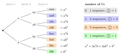
Figure 155: Multiplying out \((a+b)^3\) one factor at a time. Each factor contributes either \(a\) or \(b\), so every path from the left to a leaf is one \(a,b\)-sequence of length 3, and the eight leaves are all eight of them. The colour of a leaf is its number of \(b\)’s, and a sequence with \(k\) \(b\)’s equals \(a^{3-k}b^k\). There is 1 sequence with no \(b\), 3 with one, 3 with two and 1 with three, which are the numbers of ways to choose where the \(b\)’s go: \(\binom30, \binom31, \binom32, \binom33\). Collecting them gives \((a+b)^3 = a^3 + 3a^2b + 3ab^2 + b^3\).
The Binomial Theorem
The Binomial Theorem. For any \(a, b \in \mathbb{R}\) and any nonnegative integer \(n\), \[(a + b)^n = \sum_{k=0}^{n} \binom{n}{k} a^{n-k} b^k = a^n + \binom{n}{1} a^{n-1}b^1 + \cdots + \binom{n}{n-1} a^1 b^{n-1} + b^n.\]
The statement is printed on the exam formula-sheet; the proof is not.
Combinatorial proof. \((a+b)^n\) is the sum of all the \(a,b\)-sequences of length \(n\) (above). Group them by their number of \(b\)’s.
- A sequence with exactly \(k\) \(b\)’s has \(n - k\) \(a\)’s, so it equals \(a^{n-k}b^k\).
- How many sequences of length \(n\) have exactly \(k\) \(b\)’s? Such a sequence is fixed by choosing which \(k\) of its \(n\) positions hold a \(b\); the rest hold \(a\). So there are \(\binom{n}{k}\) of them.
- So the term \(a^{n-k}b^k\) appears \(\binom{n}{k}\) times, and \(k\) can be anything from 0 to \(n\). Adding up gives \((a+b)^n = \sum_{k=0}^{n} \binom{n}{k} a^{n-k}b^k\). \(\square\)
The end terms fit the pattern: \(a^n\) is the single sequence with no \(b\)’s, coefficient \(\binom{n}{0} = 1\), and \(b^n\) is the single sequence of all \(b\)’s, coefficient \(\binom{n}{n} = 1\).
An example to hold onto: \((a+b)^5\) and \(a^3b^2\). The sequences of length 5 with three \(a\)’s and two \(b\)’s are
\[aaabb,\ aabab,\ aabba,\ abaab,\ ababa,\ abbaa,\ baaab,\ baaba,\ babaa,\ bbaaa,\]
ten of them, so the expansion of \((a+b)^5\) contains \(10a^3b^2\). Ten is \(\binom52\), the number of ways to choose the 2 positions for the \(b\)’s out of 5. Choosing the 3 positions for the \(a\)’s instead gives \(\binom53\), which is also 10: placing the \(a\)’s settles where the \(b\)’s go, and that is the symmetry again. The full expansion is
\[(a+b)^5 = a^5 + 5a^4b + 10a^3b^2 + 10a^2b^3 + 5ab^4 + b^5,\]
with row 5 of Pascal’s triangle as its coefficients.
Figure 156: The ten \(a,b\)-sequences of length 5 with two \(b\)’s, each drawn as five positions with the two \(b\)’s shaded. A sequence is decided by which two positions hold its \(b\)’s, and every pair of positions from \({1, \dots, 5}\) appears exactly once, so there are \(\binom52 = 10\) sequences, each equal to \(a^3b^2\), and \((a+b)^5\) contains \(10a^3b^2\). The pairs are the ten 2-element subsets of \({1, 2, 3, 4, 5}\), and the \(a\)’s sit in the complementary 3 positions, so choosing the \(a\)-positions instead counts the same ten sequences as \(\binom53\).
Another way to see step 2. Multiplying out the product means choosing, from each of the \(n\) factors \((a + b)\), either its \(a\) or its \(b\). A term equal to \(a^{n-k}b^k\) comes from choosing \(b\) from some \(k\) of the factors and \(a\) from the rest, and there are \(\binom{n}{k}\) ways to choose which \(k\) factors. The positions in the sequence and the factors in the product are the same thing.
Finding a coefficient in an expansion
To find the coefficient of one power of \(x\) in something like \((3x - 2)^5\), don’t expand the whole thing. Find the one term of the Binomial Theorem that contains that power.
- Match to \((a + b)^n\), signs and constants included. In \((3x - 2)^5\), \(a = 3x\), \(b = -2\) and \(n = 5\). The minus sign belongs to \(b\), and the 3 belongs to \(a\).
- Write the general term \(\binom{n}{k} a^{n-k} b^k\) with these substituted: \(\binom5k (3x)^{5-k}(-2)^k\).
- Find \(k\). Work out the power of \(x\) in the general term as a function of \(k\), set it equal to the power wanted, and solve. Here \(x\) is inside \(a\), so it is raised to \(5 - k\). For \(x^2\), \(5 - k = 2\), so \(k = 3\).
- Substitute \(k\) and simplify, keeping the constants and the sign. \(\binom53 (3x)^2 (-2)^3 = 10 \cdot 9x^2 \cdot (-8) = -720x^2\). The coefficient is \(-720\).
The question “what should \(k\) be?” always has the same answer: whatever makes the power of \(x\) come out right. Where \(x\) sits decides the equation.
- \(x\) in the first term, \(a\). Its power is \(n - k\). So for \(x^3\) in \((x + 9)^7\), \(7 - k = 3\) and \(k = 4\).
- \(x\) in the second term, \(b\). Its power is \(k\). So for \(x^8\) in \((3 - x)^{12}\), \(a = 3\), \(b = -x\) and \(k = 8\) directly.
- \(x\) in both terms. Collect the powers. In \(\left(x^2 + \frac{1}{x}\right)^5\) the general term is \(\binom5k (x^2)^{5-k} (x^{-1})^k = \binom5k x^{10 - 3k}\). For \(x^4\), \(10 - 3k = 4\) gives \(k = 2\), and the coefficient is \(\binom52 = 10\). For \(x^5\), \(10 - 3k = 5\) has no whole-number solution, so there is no \(x^5\) term and its coefficient is 0.
Which letter is called \(a\) and which \(b\) is a free choice. Swapping them changes \(k\) to \(n - k\), and \(\binom{n}{k} = \binom{n}{n-k}\), so the answer is the same either way. What must stay consistent is that the power \(n - k\) goes on whatever was called \(a\) and the power \(k\) on whatever was called \(b\).
| Expansion | \(a\) | \(b\) | Power of \(x\) in the general term | Wanted | \(k\) | Term | Coefficient |
|---|---|---|---|---|---|---|---|
| \((x + 9)^7\) | \(x\) | \(9\) | \(7 - k\) | \(x^3\) | 4 | \(\binom74 x^3 9^4\) | \(35 \cdot 6561 = 229\,635\) |
| \((3 - x)^{12}\) | \(3\) | \(-x\) | \(k\) | \(x^8\) | 8 | \(\binom{12}{8} 3^4 (-x)^8\) | \(495 \cdot 81 = 40\,095\) |
| \((3x - 2)^5\) | \(3x\) | \(-2\) | \(5 - k\) | \(x^2\) | 3 | \(\binom53 (3x)^2 (-2)^3\) | \(10 \cdot 9 \cdot (-8) = -720\) |
These three are worked in full in 2026-10-19-probability-binomial-coefficients.
Signs. With \(b = -c\), the general term carries \((-1)^k\). It is positive when \(k\) is even and negative when \(k\) is odd. In \((3 - x)^{12}\), \((-x)^8 = x^8\), so the \(x^8\) coefficient is positive. In \((3x - 2)^5\), \((-2)^3 = -8\), so the \(x^2\) coefficient is negative.
Scaled terms. \((3x)^2 = 9x^2\), not \(3x^2\). The constant inside the bracket is raised to the power too.
The sum of a row: \(\sum_{r=0}^{n} \binom{n}{r} = 2^n\)
For every nonnegative integer \(n\), \[\sum_{r=0}^{n} \binom{n}{r} = \binom{n}{0} + \binom{n}{1} + \cdots + \binom{n}{n} = 2^n.\]
Combinatorial proof. Count the subsets of \(N = \{1, 2, \dots, n\}\) in two ways.
- All at once. The number of subsets of \(N\) is the size of its power set, \(|\mathcal{P}(N)| = 2^{|N|} = 2^n\) (sets-and-set-notation). To see why, write each subset as a 01-sequence of length \(n\): put a 1 in position \(i\) if \(i\) is in the subset and a 0 if it isn’t. For \(N = \{1, \dots, 6\}\), the sequence \(011001\) is the subset \(\{2, 3, 6\}\). Every subset gives one 01-sequence and every 01-sequence gives one subset, and there are \(2^n\) 01-sequences of length \(n\), since each position is 0 or 1.
- By size. Every subset has some cardinality \(k\) between 0 and \(n\), and the subsets of cardinality \(k\) are the 01-sequences with exactly \(k\) ones. Such a sequence is fixed by choosing which \(k\) positions hold the ones, so there are \(\binom{n}{k}\) of them. Adding over all sizes, the number of subsets is \(\sum_{k=0}^{n} \binom{n}{k}\).
Both count the subsets of \(N\), so \(2^n = \sum_{r=0}^{n} \binom{n}{r}\). \(\square\)
Figure 157: The eight subsets of \({1, 2, 3}\), each written as a 01-sequence, where a 1 in position \(i\) means \(i\) is in the subset. Grouped by size there are \(\binom30 = 1\) with no elements, \(\binom31 = 3\) with one, \(\binom32 = 3\) with two and \(\binom33 = 1\) with three: a subset of size \(k\) is a choice of \(k\) positions for the 1s. Counted all at once there are \(2^3 = 8\), two choices for each position. So row 3 of Pascal’s triangle adds up to \(2^3\).
A check from the Binomial Theorem. Put \(a = b = 1\): \((1 + 1)^n = \sum_{k=0}^{n} \binom{n}{k} 1^{n-k} 1^k\), which is the same identity. With \(a = 1\) and \(b = -1\) instead, \(0 = (1 - 1)^n = \sum_{k=0}^{n} (-1)^k \binom{n}{k}\) for \(n \ge 1\): the alternating sum of a row is 0, as in \(1 - 4 + 6 - 4 + 1 = 0\). That alternating sum is what makes inclusion-exclusion count every element exactly once.
Common mistakes
- Leaving the constant behind. In \((3x - 2)^5\) the term is \(\binom53 (3x)^2(-2)^3\), and \((3x)^2 = 9x^2\). Writing \(3x^2\) gives \(-240\) in place of \(-720\).
- Dropping the sign. The \(-\) belongs to \(b\), so it is raised to the power \(k\): \((-2)^3 = -8\) but \((-x)^8 = +x^8\). Forgetting it gives \(+720\) for the \(x^2\) coefficient of \((3x - 2)^5\).
- Putting \(k\) on the wrong letter. When \(x\) is in \(a\), its power is \(n - k\), not \(k\). In \((x + 9)^7\), solving \(k = 3\) and then writing \(\binom73 x^4 9^3\) finds the \(x^4\) coefficient, not the \(x^3\) one. The binomial \(\binom73 = \binom74\) is the same either way; the powers on \(a\) and \(b\) are what go wrong.
- Expecting every power to appear. In \(\left(x^2 + \frac1x\right)^5\) the powers are \(x^{10 - 3k}\), so \(x^5\) never appears and its coefficient is 0. A \(k\) that is not a whole number between 0 and \(n\) means the term isn’t there.
- Pascal’s formula with the wrong indices. It is \(\binom{n+1}{r} = \binom{n}{r-1} + \binom{n}{r}\): the two entries diagonally above, both from row \(n\). Not \(\binom{n}{r} + \binom{n}{r+1}\) in row \(n+1\), and not two entries from different rows.
- Treating two groups as a product. Splitting 400 people into groups of 150 and 250 is \(\binom{400}{150}\), not \(\binom{400}{150}\binom{400}{250}\): once the 150 are chosen the other group is already decided. (If it were written as stages, the second stage would be \(\binom{250}{250} = 1\).)
- A combinatorial proof that only computes. Showing \(84 = 28 + 56\) checks one case. The proof has to say what is being counted and why each side counts it.
See also
- counting-selections — \(n\) choose \(r\) as the count of subsets, its formula, and the other three kinds of selection
- counting-principles — the addition and multiplication rules that the combinatorial proofs use
- [probability] — probabilities worked out by counting, many of them with binomial coefficients
- sets-and-set-notation — subsets, complements and the power set
- inclusion-exclusion — counting a union, which rests on the alternating row sum
- 2026-10-19-probability-binomial-coefficients — Lecture 31
- practice-problems — §40, coefficients in expansions, with full worked solutions
Cardinality
What it means for two sets to be the same size, and how to compare the sizes of sets that are infinite. It all comes down to functions: same size means there is a bijection, and no bigger means there is an injection. The one-to-one, onto and bijection machinery is in one-to-one-and-onto-functions. Which infinite sets can be listed, and which cannot, is in countable-and-uncountable-sets. The lectures are 2026-09-14-cardinalities and 2026-09-15-countable-and-uncountable-sets.
Same size means a bijection
Any two sets have the same cardinality if and only if there is a bijection between them. If the sets \(A\) and \(B\) have the same cardinality, then we write \(|A| = |B|\).
This is a definition, and it is the same idea as counting. Counting a finite set means pairing its elements off with \(1, 2, \dots, n\), so “\(A\) has \(n\) elements” says \(|A| = |\{1, 2, \dots, n\}|\). For finite sets the definition therefore agrees with counting:
Any two finite sets have the same number of elements if and only if there is a bijection between them.
The definition drops only the requirement that the pairing stop. That is what makes it work for infinite sets, and also what makes it surprising there.
Because bijections can be inverted and composed (inverse-functions, composition-of-functions), “same cardinality” behaves like equality. Every set has the same cardinality as itself (the identity). If \(|A| = |B|\) then \(|B| = |A|\) (the inverse). If \(|A| = |B|\) and \(|B| = |C|\) then \(|A| = |C|\) (the composite). That is what lets results be chained, as in \(|\mathbb{Z}^{+}| = |\mathbb{Z}| = |\mathbb{Q}|\).
Finite sets
For finite sets \(A\) and \(B\):
- If \(A\) has more elements than \(B\), there is no one-to-one function \(f : A \to B\).
- If \(A\) has fewer elements than \(B\), there is no onto function \(f : A \to B\).
- If \(A\) and \(B\) have the same number of elements, then any function \(f : A \to B\) is one-to-one if and only if it is onto.
- When \(A\) and \(B\) have the same number of elements there can still be functions from \(A\) to \(B\) that are neither.
Figure 158: The four facts about finite sets, each with the counting reason. (1) With more elements in \(A\) than in \(B\), the arrows run out of fresh targets: once every dot of \(B\) is used, the next arrow must share one. (2) With fewer elements in \(A\), there are not enough arrows to reach every dot of \(B\). (3) With equal numbers, merging two arrows is the same thing as missing a target, so one-to-one and onto stand or fall together. (4) Equal numbers do not force either property, only their agreement: this function merges two arrows and so misses one dot.
Fact 1 is the pigeonhole principle in function form, a name the course reaches later in the semester (pigeonhole-principle). Fact 3 is the useful one in practice. Between two finite sets of the same size, checking one of one-to-one and onto is enough.
Fact 3 is false for infinite sets. On \(\mathbb{Z}^{+}\):
- \(f(n) = 2n\) is one-to-one but not onto (nothing maps to 1);
- \(g(n) = \lceil n/2 \rceil\) is onto but not one-to-one (\(g(1) = g(2) = 1\)).
Both go from a set to itself, so the two sides certainly have the same cardinality. For infinite sets one-to-one and onto have to be checked separately, every time.
Infinite sets break the finite intuition
For finite sets a proper subset is always strictly smaller. For infinite sets it need not be:
| Set | Proper subset | Bijection |
|---|---|---|
| \(\mathbb{Z}^{+}\) | \(2\mathbb{Z}^{+}\) (even positive integers) | \(n \mapsto 2n\) |
| \(\mathbb{Z}^{+}\) | \(\mathbb{Z}^{+} - \{1\}\) | \(n \mapsto n + 1\) |
| \(\mathbb{Z}\) | \(\{n \in \mathbb{Z} : n \bmod 3 = 1\}\) | \(n \mapsto 3n + 1\) |
Sets that look very different in size can match up too. \(\mathbb{Z}^{+}\) pairs off with all of \(\mathbb{Z} \times \mathbb{Z}\) along a spiral (2026-09-14-cardinalities), and the short interval \([0,1]\) with the long interval \([6,9]\) by projection (2026-09-15-countable-and-uncountable-sets).
This is the point of Hilbert’s Hotel (2026-09-14-cardinalities). A full hotel with infinitely many rooms can take one more guest, or a busload, or infinitely many busloads, by moving everyone, because \(\mathbb{Z}^{+}\) can be put in one-to-one correspondence with a proper part of itself.
“Clearly \(|\mathbb{Q}| > |\mathbb{Z}| > |\mathbb{Z}^{+}|\)” is the containment intuition applied where it no longer holds. Containment gives \(\leq\) (the inclusion map is an injection, see below), never automatically \(<\).
Beyond the course: this property characterises infinite sets. A set is infinite exactly when it has the same cardinality as some proper subset of itself.
Proving \(|X| = |Y|\)
The template, used in 2026-09-14-cardinalities:
One way to show \(|X| = |Y|\) for sets \(X\) and \(Y\):
- Define a function \(f : X \to Y\) and explain why it is a function (each element of \(X\) has a unique image in \(Y\)).
- Show \(f\) is one-to-one (injective).
- Show \(f\) is onto (surjective).
Step 1 is where most of the real checking happens. \(f(x)\) has to land in \(Y\), not merely somewhere. In step 3 the preimage you construct has to be in \(X\). Both are range checks, and both use the definitions of \(X\) and \(Y\).
Worked: \(|\mathbb{Z}^{+}| = |\mathbb{Z}|\)
The listing \(0, 1, -1, 2, -2, 3, -3, \dots\) (drawn in countable-and-uncountable-sets) as a formula:
\[f : \mathbb{Z}^{+} \to \mathbb{Z}, \qquad f(n) = \begin{cases} \dfrac{n}{2} & n \text{ even,} \\[6pt] -\dfrac{n-1}{2} & n \text{ odd.} \end{cases}\]
It is a function into \(\mathbb{Z}\). Every \(n \in \mathbb{Z}^{+}\) is even or odd, not both, so exactly one case applies. If \(n\) is even, \(\frac{n}{2} \in \mathbb{Z}\). If \(n\) is odd, \(n - 1\) is even and \(-\frac{n-1}{2} \in \mathbb{Z}\).
One-to-one. Suppose \(f(n_1) = f(n_2)\). The even case gives values \(\geq 1\), and the odd case gives values \(\leq 0\), so \(n_1\) and \(n_2\) fall in the same case. If both are even, \(\frac{n_1}{2} = \frac{n_2}{2}\) gives \(n_1 = n_2\). If both are odd, \(-\frac{n_1 - 1}{2} = -\frac{n_2 - 1}{2}\) gives \(n_1 = n_2\).
Onto. Let \(m \in \mathbb{Z}\). If \(m \geq 1\), take \(n = 2m\), a positive even integer, and \(f(2m) = m\). If \(m \leq 0\), take \(n = 1 - 2m\), a positive odd integer, and \(f(1 - 2m) = -\frac{(1-2m)-1}{2} = m\).
So \(f\) is a bijection and \(|\mathbb{Z}^{+}| = |\mathbb{Z}|\). \(\square\)
The case split in the one-to-one step is the part to notice. With a function defined by cases, first show the two inputs must be in the same case, here by comparing the values each case can produce. Then argue within the case.
Comparing sizes: injections and surjections
For any sets \(A\) and \(B\):
\(|A| \leq |B| \leftrightarrow \exists\) injective \(f : A \to B\).
\(|A| \geq |B| \leftrightarrow \exists\) surjective \(f : A \to B\).
\(|A| < |B| \leftrightarrow \exists\) injective \(f : A \to B\) but \(\nexists\) bijective \(f : A \to B\).
\(|A| > |B| \leftrightarrow \exists\) surjective \(f : A \to B\) but \(\nexists\) bijective \(f : A \to B\).
Both definitions are the finite facts turned round. An injection fits \(A\) inside \(B\) without collisions, so \(B\) has at least as much room. A surjection covers \(B\) using \(A\), so \(A\) has at least as much to spend. The functions witnessing \(\leq\) and \(\geq\) need not be the same function, and usually are not.
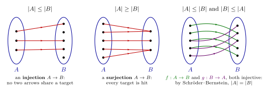
Figure 159: The three comparisons as functions. Left: an injection fits \(A\) inside \(B\) with no collisions, so \(|A| \leq |B|\); some of \(B\) may be left over. Middle: a surjection covers all of \(B\) using \(A\), so \(|A| \geq |B|\); arrows may double up. Right: an injection each way, \(f : A \to B\) and a different \(g : B \to A\). Neither need be onto, but by the Schröder–Bernstein Theorem together they guarantee that some bijection exists, so \(|A| = |B|\).
(The rightmost panel is drawn with finite sets only to show the shape of the argument. For finite sets an injection each way already forces equal sizes by counting. The theorem is needed, and is surprising, only for infinite sets.)
Two consequences used all the time:
- A subset is never bigger. If \(A \subseteq B\) then \(|A| \leq |B|\), by the inclusion map \(a \mapsto a\), which is injective. This is all that “\(\mathbb{Z}^{+} \subset \mathbb{Q}\)” proves about sizes.
- A list of things is never bigger than \(\mathbb{Z}^{+}\). If \(x_1, x_2, x_3, \dots\) is any sequence, then \(i \mapsto x_i\) is onto the set \(\{x_1, x_2, x_3, \dots\}\), so that set has cardinality \(\leq |\mathbb{Z}^{+}|\). The set is countable, whether or not the sequence repeats (2026-09-15-countable-and-uncountable-sets).
Beyond the course: the surjection definition of \(\geq\) needs one exception. There is no function at all from a non-empty set to \(\emptyset\), so \(|A| \geq |\emptyset|\) has no surjection behind it, yet it is plainly true. Read the surjection definition as being about non-empty \(B\).
The Schröder–Bernstein Theorem
The Schröder–Bernstein Theorem. For all sets \(A\) and \(B\), if \(|A| \leq |B|\) and \(|A| \geq |B|\), then \(|A| = |B|\).
It is on the formula sheet (formula-sheet). In practice it is used in this form:
To show \(|A| = |B|\), instead of finding a bijection from \(A\) to \(B\), you can find a function that shows \(|A| \leq |B|\) and a different function that shows \(|B| \leq |A|\).
That is, one injection each way. The two injections do not have to fit together, and neither has to be onto. It is the right tool when a bijection would be fiddly, typically because of endpoints or because the sets are built differently.
Worked: \(|[0,1)| = |[0,1]|\)
A bijection between these two exists but has to do something awkward to make room for the extra endpoint. Two injections are easy:
- \(f : [0,1) \to [0,1]\), \(f(x) = x\). It lands in \([0,1]\) because \([0,1) \subseteq [0,1]\), and it is one-to-one because \(f(x_1) = f(x_2)\) says \(x_1 = x_2\). So \(|[0,1)| \leq |[0,1]|\).
- \(g : [0,1] \to [0,1)\), \(g(x) = \frac{x}{2}\). If \(0 \leq x \leq 1\) then \(0 \leq \frac{x}{2} \leq \frac{1}{2} < 1\), so it lands in \([0,1)\). \(\frac{x_1}{2} = \frac{x_2}{2}\) gives \(x_1 = x_2\). So \(|[0,1]| \leq |[0,1)|\).
By the Schröder–Bernstein Theorem, \(|[0,1)| = |[0,1]|\). \(\square\)
Same shape as the proof that \(|[0,1]| = |(6,9)|\) (2026-09-15-countable-and-uncountable-sets), and as the proof that \(\mathbb{Z}^{+} \times \mathbb{Z}^{+}\) is countable, which uses the injections \((a,b) \mapsto 3^a 5^b\) and \(n \mapsto (n,1)\).
The direction trap
Both inequalities must be about the same pair in opposite directions. The trap is in the directions:
- an injection \(X \to Y\) and a surjection \(X \to Y\) — gives \(|X| \leq |Y|\) and \(|X| \geq |Y|\), sufficient;
- an injection \(X \to Y\) and a surjection \(Y \to X\) — gives \(|X| \leq |Y|\) and \(|Y| \geq |X|\), the same fact twice, not sufficient.
Before invoking the theorem, write out the two inequalities the functions give and check that one is \(\leq\) and the other is \(\geq\) between the same two sets in the same order.
Common mistakes
- Reading size off containment. \(A \subsetneq B\) proves \(|A| \leq |B|\), never \(|A| < |B|\), when the sets are infinite.
- Skipping the range check. A formula is not a function into \(Y\) until you have shown every value lies in \(Y\) — \(3n + 1 \in S\), \(6 \leq 3x + 6 \leq 9\).
- Proving only one of one-to-one and onto. Enough for finite sets of equal size (fact 3), never enough for infinite ones.
- Using Schröder–Bernstein with the arrows the wrong way round. See the direction trap above.
- Proving a set is not the same size by failing to find a bijection. Not finding one proves nothing. That \(\mathbb{R}\) is not the size of \(\mathbb{Z}^{+}\) takes an argument that no list can work, the diagonal argument in countable-and-uncountable-sets.
See also
- countable-and-uncountable-sets — finite, countable and uncountable sets; listing arguments; the diagonal argument
- one-to-one-and-onto-functions — the definitions and proof templates every argument here uses
- inverse-functions · composition-of-functions — why “same cardinality” chains like equality
- formula-sheet — the Schröder–Bernstein Theorem as printed on the exam formula page
- counting-principles — counting finite sets without listing them, by the multiplication and addition rules
- pigeonhole-principle — fact 1 put to work: choosing the pigeons and the holes to prove that two chosen things must coincide
- 2026-09-14-cardinalities — Lecture 21 · 2026-09-15-countable-and-uncountable-sets — Lecture 22
- practice-problems — §27, with full worked solutions
Cayley Tables
A Cayley table writes out every product in a finite set with an operation. For a group, most of the definition can be read straight off it. The definition is in [groups]. The tables for \(\mathbb{Z}_7 - \{[0]\}\) and for \(S_3\) are built in 2026-09-24-definitions-and-examples-of-groups. With the right ordering of the headings, a subgroup shows up as a block of the table (below, and subgroups-and-cyclic-groups).
What a Cayley table is
One row and one column for each element, in the same order, with the operation’s symbol in the corner. The entry in the row of \(g\) and the column of \(h\) is \(g * h\): row first, then column.
The order matters whenever the operation is not commutative. In the table of \(S_3\) the entry in row \(f_2\), column \(f_3\) is \(f_6\), so \(f_2 \circ f_3 = f_6\) (2026-09-24-definitions-and-examples-of-groups). The entry in row \(f_3\), column \(f_2\) is a different element, \(f_5\).
Reading the properties off a table
| Property | What to look for in the table |
|---|---|
| closure | The body uses only the elements in the headings. |
| associativity | Cannot be seen. It has to be argued separately, or be given. |
| identity | A row that repeats the column headings and a column that repeats the row headings, belonging to the same element. |
| inverses | The identity \(e\) appears in every row. If \(e\) is in row \(g\) and column \(h\), then \(g * h = e\). |
| abelian | The table is its own mirror image in the main diagonal (top left to bottom right). |
For \(\mathbb{Z}_7 - \{[0]\}\) the checks read: closure, because the body of the table uses only \([1], \dots, [6]\); associativity, given; identity \([1]\), since \([1] \cdot g = g \cdot [1] = g\); and six inverses, one from each \([1]\) in the body (2026-09-24-definitions-and-examples-of-groups).
Three details:
- Identity needs the row and the column. The row of \(e\) shows \(e * g = g\), and the column shows \(g * e = g\). The definition asks for both.
- Inverses need both orders too. \(g * h = e\) and \(h * g = e\) are two different cells, mirror images of each other. So the \(e\)s in a group’s table are placed symmetrically about the diagonal, even when the table as a whole is not symmetric. In \(S_3\), \(f_5 \circ f_6 = f_1\) and \(f_6 \circ f_5 = f_1\).
- An \(e\) on the diagonal means an element is its own inverse. In \(\mathbb{Z}_7 - \{[0]\}\) those are \([1]\) and \([6]\).
The figure below marks the same three things on a second table, the one for \(\mathbb{Z}_5 - \{[0]\}\) from practice-problems, Q4.
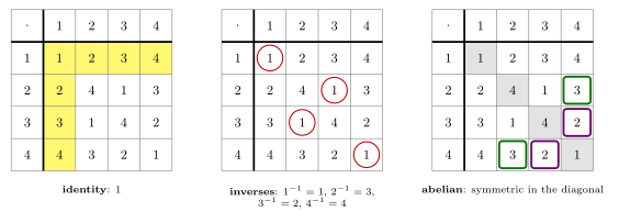
Figure 160: Three readings of one table, \(\mathbb{Z}_5 - {[0]}\) under multiplication, written without brackets. Left: the row and the column of 1, in yellow, repeat the headings, so 1 is the identity. Middle: the identity appears once in every row. The ring in row 2 is in column 3, so \(2^{-1} = 3\); the rings on the diagonal show that 1 and 4 are their own inverses. Right: each entry equals its mirror image in the shaded diagonal, such as the two boxed 3s and the two boxed 2s, so the operation is commutative and the group is abelian.
Rows and columns have no repeats
In a Cayley table for a group, the elements in each row are distinct.
A similar argument shows that the elements in each column are distinct.
Rows. By contradiction (2026-09-24-definitions-and-examples-of-groups). Suppose row \(a\) has the same entry \(x\) in two different columns \(b \neq c\), so \(a * b = a * c\). Apply \(a^{-1}\) on the left of both sides:
\[a^{-1} * (a * b) = a^{-1} * (a * c) \ \Longrightarrow\ (a^{-1} * a) * b = (a^{-1} * a) * c \ \Longrightarrow\ e * b = e * c \ \Longrightarrow\ b = c,\]
using inverses, associativity, inverses and identity in turn. That contradicts \(b \neq c\). \((\Rightarrow\Leftarrow)\)
Columns. The “similar argument”, written out. Suppose column \(a\) has the same entry in two different rows \(b \neq c\), so \(b * a = c * a\). Now \(a\) is on the right, so apply \(a^{-1}\) on the right:
\[(b * a) * a^{-1} = (c * a) * a^{-1} \ \Longrightarrow\ b * (a * a^{-1}) = c * (a * a^{-1}) \ \Longrightarrow\ b * e = c * e \ \Longrightarrow\ b = c,\]
a contradiction again. The figure below shows both cases.
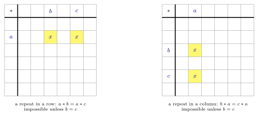
Figure 161: What the two results forbid. Left: the same element \(x\) twice in the row of \(a\), in the columns of two different elements \(b\) and \(c\). That would mean \(a * b = a * c\), and applying \(a^{-1}\) on the left gives \(b = c\). Right, the column version: the same \(x\) twice in the column of \(a\), which would mean \(b * a = c * a\), and applying \(a^{-1}\) on the right gives \(b = c\). Neither picture can occur in the table of a group.
The two results are cancellation: from \(a * b = a * c\) conclude \(b = c\), and from \(b * a = c * a\) conclude \(b = c\). The \(a\) being cancelled must be on the same side in both products. \(a * b = c * a\) does not give \(b = c\) unless the group is abelian.
What it gives for a finite table
In a group with \(n\) elements, a row has \(n\) entries, all different, all taken from the \(n\) elements. So every element appears exactly once in every row, and likewise in every column. Check it against the tables for \(\mathbb{Z}_7 - \{[0]\}\) and \(S_3\). Three uses:
- Finishing a table. A row with one empty cell must be completed by the one element not yet in it. Suppose the last row of the \(S_3\) table has only \(f_5\) filled in, in its last cell, and the other five cells empty. Once four of them are worked out, \(f_6, f_4, f_2, f_3\), the remaining one must be \(f_1\).
- Spotting a non-group. A repeat in a row or a column means the table is not a group’s. Multiplication mod 9 on \(\{1, \dots, 8\}\) has \(3 \cdot 1 = 3\) and \(3 \cdot 4 = 12 \equiv 3\) in the row of 3. That set is also not closed, since \(3 \cdot 3 \equiv 0\) (practice-problems, Q1).
- Finding inverses. \(e\) appears exactly once in each row, so each element has exactly one inverse to read off.
No repeats does not show that a table is a group’s. Associativity still cannot be seen in a table.
Subgroups in a table
A subgroup is a subset that is a group under the same operation (subgroups-and-cyclic-groups). To see one in a table, list its elements first, in the same order along the top and down the side. Then the top-left block of the table holds every product of two of its elements: it is the subgroup’s own table, and the checks are read off the block.
| Check | What to look for in the block |
|---|---|
| closure | The body of the block uses only the block’s own headings. |
| identity | The identity of the group is among the block’s headings. |
| inverses | The identity appears in every row of the block. |
| associativity | Nothing to check: it is inherited from the whole group. |
\((\mathbb{Z}_6, +)\) with \([0], [2], [4]\) listed first is drawn in 2026-10-06-elementary-properties-of-groups. The same works in a non-abelian group. In \(S_3\), list \(f_1, f_5, f_6\) first:
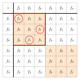
Figure 162: The Cayley table of \(S_3\) with \(f_1, f_5, f_6\) listed first; the entry in the row of \(f\) and the column of \(g\) is \(f \circ g\). The outlined top-left block uses only \(f_1, f_5, f_6\), so that set is closed under composition. It contains the identity \(f_1\), and the rings show \(f_1\) in every row of the block, so each of the three has its inverse among them: \(f_5 \circ f_6 = f_6 \circ f_5 = f_1\). So \({f_1, f_5, f_6}\) is a subgroup of \(S_3\). Shaded cells hold \(f_1\), \(f_5\) or \(f_6\). As with the even classes of \(\mathbb{Z}_6\), the table falls into four blocks, each using only the subgroup’s elements or only the other three.
\(\{f_1, f_5, f_6\}\) is every power of \(f_5\), since \(f_5^2 = f_6\) and \(f_5^3 = f_1\), so it is the cyclic subgroup \(\langle f_5 \rangle\) (symmetric-group).
A subset that is not a subgroup leaks. List \(f_1, f_2, f_3\) first instead. The block then contains \(f_2 \circ f_3 = f_6\), which is not one of its headings, so \(\{f_1, f_2, f_3\}\) is not closed and is not a subgroup. In \(\mathbb{Z}_6\), the block for \(\{[0], [1]\}\) contains \([1] + [1] = [2]\), and fails the same way.
The tables in the course so far
| Group | Elements | Abelian? | Where |
|---|---|---|---|
| \((\mathbb{Z}_7 - \{[0]\}, \cdot)\) | 6 | yes | 2026-09-24-definitions-and-examples-of-groups |
| \((S_3, \circ)\) | 6 | no | 2026-09-24-definitions-and-examples-of-groups |
| \((\mathbb{Z}_5 - \{[0]\}, \cdot)\) | 4 | yes | practice-problems, Q4; above |
| \((\mathbb{Z}_2 \times \mathbb{Z}_2, +)\) | 4 | yes | the same practice set, Q5 |
| \((\mathbb{Z}_3, +)\) | 3 | yes | integers-modulo-n |
| \((\mathbb{Z}_6, +)\), even classes first | 6 | yes | 2026-10-06-elementary-properties-of-groups |
| \((S_3, \circ)\), \(f_1, f_5, f_6\) first | 6 | no | above |
The first two have the same number of elements and are different kinds of group: one is abelian and the other is not. The size of a group does not determine it.
Common mistakes
- Reading the entry as column \(*\) row. It is row \(*\) column. For an abelian group the mistake is invisible. For \(S_3\) it gives wrong answers.
- Listing the rows and columns in different orders. The diagonal symmetry test needs the same order on both.
- Claiming the identity from its row alone.
- “The table has no repeats, so it is a group.” Closure, identity and inverses can be read off. Associativity cannot.
- Forgetting closure. An entry in the body that is not one of the headings ends the matter at once.
See also
- [groups] — the four properties the table is checked against, and cancellation as solving \(a * x = b\)
- integers-modulo-n — the groups \(\mathbb{Z}_n\) and \(\mathbb{Z}_n - \{[0]\}\) behind the first tables
- symmetric-group — \(S_3\), whose table is not symmetric
- subgroups-and-cyclic-groups — subgroups and cyclic subgroups, the blocks found above
- proof-techniques — proof by contradiction, the method of the rows result
- 2026-09-24-definitions-and-examples-of-groups — Lecture 26 · 2026-10-06-elementary-properties-of-groups — Lecture 27 · 2026-10-08-definitions-and-examples-of-fields — Lecture 28, where the table of \(\mathbb{Z}_4 - \{[0]\}\) fails closure
- practice-problems — §33, with full worked solutions
Composition of Functions
Chaining two functions into one, and which properties survive the chaining — in both directions. First met in 2026-09-08-composition-of-functions; the properties are defined in one-to-one-and-onto-functions and inverse-functions.
Definition
Let \(f : X \to Y\) and \(g : Y \to Z\) be functions. The composition of \(f\) and \(g\) is the function \(g \circ f : X \to Z\) defined by \[(g \circ f)(x) = g(f(x)) \quad\text{for all } x \in X.\]
Three things to read off the definition:
- Right to left. \(g \circ f\) applies \(f\) first, then \(g\). The order of the symbols matches the formula \(g(f(x))\), not the order of events.
- The domain of \(g \circ f\) is the domain of \(f\); the co-domain is the co-domain of \(g\). The middle set \(Y\) vanishes from the type.
- It is defined only when \(f\)’s co-domain is \(g\)’s domain. \(g \circ f\) makes sense because \(f\) lands in \(Y\) and \(g\) eats \(Y\). The other composite, \(f \circ g\), would need \(g\)’s outputs (in \(Z\)) to be inputs to \(f\) (from \(X\)), so it exists only if \(Z = X\).
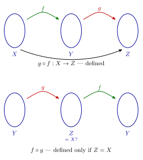
Figure 163: Why \(g \circ f\) exists and \(f \circ g\) usually does not. Top: \(f\) then \(g\) chains because \(f\) lands exactly where \(g\) starts. Bottom: \(g\) then \(f\) would need \(g\)’s outputs, in \(Z\), to be acceptable inputs to \(f\), which come from \(X\) — so it is defined only if \(Z = X\).
The composition itself is drawn in 2026-09-08-composition-of-functions: three ellipses, \(x \mapsto f(x) \mapsto g(f(x))\), with the long arrow \(g \circ f\) beneath.
Composition is not commutative. Even when both orders exist (\(X = Y = Z\)), \(g \circ f\) and \(f \circ g\) are generally different functions: with \(f(x) = x + 1\) and \(g(x) = 2x\) on \(\mathbb{R}\), \((g \circ f)(x) = 2x + 2\) but \((f \circ g)(x) = 2x + 1\).
Inverses and composition
For a bijection \(f : X \to Y\) with inverse \(f^{-1} : Y \to X\) (inverse-functions), both composites exist and both do nothing:
\[(f^{-1} \circ f)(x) = x \text{ for all } x \in X, \qquad (f \circ f^{-1})(y) = y \text{ for all } y \in Y.\]
This is the sense check on a computed inverse: for \(f((x,y)) = (y+1, 2x)\) and the claimed \(f^{-1}((x,y)) = \left(\frac{y}{2}, x - 1\right)\), \[f\!\left(f^{-1}((x,y))\right) = f\!\left(\left(\tfrac{y}{2}, x-1\right)\right) = (x, y). \;\checkmark\]
Which properties compose
Two facts:
If \(f\) and \(g\) are both onto, then \(g \circ f\) is onto. If \(f\) and \(g\) are both one-to-one, then \(g \circ f\) is one-to-one.
So both bijective gives \(g \circ f\) bijective. The proofs are short:
- Onto. Let \(z \in Z\). Since \(g\) is onto, \(\exists\, y \in Y\) with \(g(y) = z\). Since \(f\) is onto, \(\exists\, x \in X\) with \(f(x) = y\). Then \(g(f(x)) = z\). \(\square\)
- One-to-one. Suppose \(g(f(x_1)) = g(f(x_2))\). Since \(g\) is one-to-one, \(f(x_1) = f(x_2)\). Since \(f\) is one-to-one, \(x_1 = x_2\). \(\square\)
Which properties come back
The converse asks which ingredient must have a property when the composite has it. The answer is asymmetric:
| If \(g \circ f\) is … | then \(f\) must be … | then \(g\) must be … |
|---|---|---|
| onto | not necessarily | onto |
| one-to-one | one-to-one | not necessarily |
The property comes back to the function on its own side. Onto is about covering \(Z\), and \(g\) is the function that lands in \(Z\). One-to-one is about not merging elements of \(X\), and \(f\) is the function that leaves \(X\). The other ingredient can misbehave in the middle set \(Y\) without the composite noticing, as long as the misbehaviour is never exercised.
The two theorems, by contraposition
If \(g \circ f\) is onto, then \(g\) is onto.
Proof. We prove the contrapositive: if \(g\) is not onto then \(g \circ f\) is not onto. Suppose \(g\) is not onto. Then \(\exists\, z \in Z\) not in the range of \(g\). Then no \(x \in X\) has \(g(f(x)) = z\) — for if one did, \(y = f(x)\) would have \(g(y) = z\), a contradiction. So \(z\) is not in the range of \(g \circ f\), and \(g \circ f\) is not onto. \(\square\)
If \(g \circ f\) is one-to-one, then \(f\) is one-to-one.
Proof. We prove the contrapositive: if \(f\) is not one-to-one then \(g \circ f\) is not one-to-one. Suppose \(f\) is not one-to-one. Then \(\exists\, x_1 \neq x_2 \in X\) with \(f(x_1) = f(x_2)\). Hence \(g(f(x_1)) = g(f(x_2))\), i.e. \((g \circ f)(x_1) = (g \circ f)(x_2)\) with \(x_1 \neq x_2\), so \(g \circ f\) is not one-to-one. \(\square\)
Both go by contraposition (proof-techniques) for the same reason: not onto and not one-to-one are existential and hand you a concrete witness — a missed \(z\), a colliding pair — to push through the composite. The positive forms are universal and give nothing to hold onto. Anything the composite reaches, \(g\) reaches; anything \(f\) merges, the composite merges.
The two counterexamples, to order
\(g \circ f\) onto does not force \(f\) onto. \(X = \{a,b\}\), \(Y = \{0,1,2\}\), \(Z = \{v,w\}\); \(f = \{(a,0),(b,1)\}\), \(g = \{(0,v),(1,w),(2,w)\}\). Then \(f\) misses \(2\), but \(g \circ f = \{(a,v),(b,w)\}\) is onto.
\(g \circ f\) one-to-one does not force \(g\) one-to-one. \(X = \{a,b\}\), \(Y = \{1,2,3\}\), \(Z = \{u,v\}\); \(f = \{(a,1),(b,2)\}\), \(g = \{(1,u),(2,v),(3,v)\}\). Then \(g(2) = g(3)\), but \(g \circ f = \{(a,u),(b,v)\}\) is one-to-one.
Both are drawn in 2026-09-08-composition-of-functions, as (1) and (4) there, and both are built by the same recipe, which is the transferable skill:
- Make \(Y\) one element bigger than it needs to be. That spare element is where the defect will live.
- Give the defect to the function on the wrong side. For (1) \(f\) must miss the spare element; for (4) \(g\) must merge the spare element with another.
- Make sure the composite never touches it. In (1), \(g\) sends the missed element somewhere already covered, so the gap is invisible from \(Z\). In (4), \(f\) never lands on the merged element, so the collision is never fed.
- Use small sets. Two-element \(X\) and \(Z\) with a three-element \(Y\), as above, is enough; even smaller works. A counterexample is a witness; it does not need to be interesting.
The mirror symmetry is exact: (1) is gap in \(f\), hidden by a merge in \(g\); (4) is merge in \(g\), hidden by a gap in \(f\).
See also
- one-to-one-and-onto-functions — the properties and their proof templates
- inverse-functions — \(f \circ f^{-1}\) as the identity
- symmetric-group — composition as the operation of a group, on the bijections of \(\{1, \dots, n\}\)
- groups — the functions \(ax + b\) with \(a \neq 0\), a second non-abelian group under composition
- proof-techniques — contraposition and counterexample
- 2026-09-08-composition-of-functions — Lecture 20 · 2026-09-07-functions-one-to-one-onto-inverse — Lecture 19
- practice-problems — §26
Conditional & Biconditional Statements
Conditional (\(\to\))
| \(p\) | \(q\) | \(p \to q\) |
|---|---|---|
| T | T | T |
| T | F | F |
| F | T | T |
| F | F | T |
Only one row makes a conditional false: the row where the hypothesis \(p\) is true and the conclusion \(q\) is false. Everything else is true, including both rows where \(p\) is false.
\(p \to q\) is true when \(p\) is false because that is how it is defined. There is no deeper intuition to recover; \(\to\) is a truth-functional connective fixed by the table above, and arguing with the bottom two rows is arguing with a definition. The standard name for those two rows is vacuous truth. It does real work later: it is why \(\emptyset \subseteq A\) for every set \(A\) (see sets-and-set-notation).
The picture behind the table is containment:
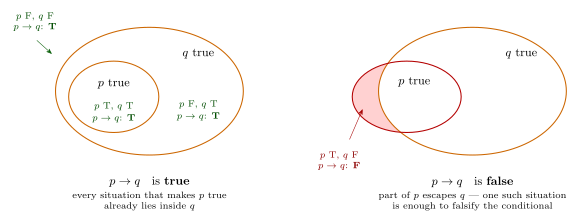
Figure 164: Why the truth table has the shape it does. Left: p → q asserts that the situations making p true all lie inside the situations making q true, so every region carries T. Right: the conditional fails exactly when part of p escapes q, which is the single F row of the table.
Disjunctive form
By definition,
\[p \to q \;\equiv\; \sim p \lor q\]
The right-hand side is the disjunctive form of the conditional, and it is the single most useful fact in the topic: the laws of logical equivalence (see logical-equivalence-laws) are stated only for \(\sim\), \(\land\) and \(\lor\), so they say nothing about \(\to\) directly. To use the laws on a conditional:
Replace \(p \to q\) with \(\sim p \lor q\) and then use the laws.
Every worked proof about conditionals in this course starts and (usually) ends with that substitution.
\(p \to q\) can be phrased: “\(p\) implies \(q\)”, “if \(p\) then \(q\)”, “\(q\) if \(p\)”, “\(p\) is sufficient for \(q\)”, “\(p\) only if \(q\)”, “\(q\) is necessary for \(p\)”.
Warning: \(p \to q \not\equiv q \to p\).
Contrapositive, converse, inverse
| Name | Form | Equivalent to |
|---|---|---|
| Conditional | \(p \to q\) | Contrapositive |
| Contrapositive | \(\sim q \to \sim p\) | Conditional |
| Converse | \(q \to p\) | Inverse |
| Inverse | \(\sim p \to \sim q\) | Converse |
The conditional and its contrapositive are always logically equivalent. The converse and inverse are always logically equivalent to each other — but not to the original conditional.
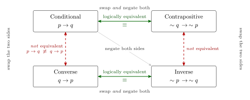
Figure 165: The four forms and the only equivalences among them. The conditional and the contrapositive are one logically equivalent pair, the converse and the inverse are the other, and p → q ≢ q → p. Swapping the two sides gives the converse, negating both gives the inverse, and doing both gives the contrapositive — the only one of the three that preserves meaning.
Both equivalences fall straight out of the disjunctive form. For the first: \(p \to q \equiv \sim p \lor q\) and \(\sim q \to \sim p \equiv \sim(\sim q) \,\lor\sim p \equiv q \,\lor\sim p\), which is the same disjunction commuted. The converse/inverse pair is the same computation with \(p\) and \(q\) interchanged.
Necessary and sufficient conditions
- \(p\) is a necessary condition for \(q\) means “if \(\sim p\) then \(\sim q\)”, or equivalently “if \(q\) then \(p\)”, or “\(q\) only if \(p\)”. In symbols, \(q \to p\).
- \(p\) is a sufficient condition for \(q\) means “if \(p\) then \(q\)”, or equivalently “\(q\) if \(p\)”. In symbols, \(p \to q\).
The two phrasings of “necessary” are contrapositives of each other, which is why they say the same thing: \(\sim p \,\to\sim q\) and \(q \to p\).
The reliable reading is: “if” introduces the sufficient condition; “only if” introduces the necessary one.
Worked: necessary but not sufficient
Being a non-negative integer is necessary for a number to be the square of an integer, but it is not sufficient.
- Necessary: if a number is the square of an integer, then it is non-negative. So \(-9\) cannot be the square of an integer — failing the condition rules the number out.
- Not sufficient: \(7\) is a non-negative integer but it is not the square of an integer. Meeting the condition does not settle it.
Worked: sufficient but not necessary
Being an integer that is divisible by 4 is sufficient for being an even integer, but it is not necessary.
- Sufficient: if an integer is divisible by 4, then it is even. \(8\) is divisible by 4, so we know \(8\) is even without checking anything else.
- Not necessary: \(10\) is an even integer but \(10\) is not divisible by 4. The condition can fail while the conclusion still holds.
The two shapes are exactly opposite in how they are refuted: a claimed sufficient condition is killed by something satisfying the condition but not the conclusion; a claimed necessary condition is killed by something satisfying the conclusion but not the condition.
Biconditional (\(\leftrightarrow\))
\[a \leftrightarrow b \equiv (a \to b) \land (b \to a)\]
A biconditional is the two one-way conditionals conjoined, and each of the standard English phrasings splits along the same seam:
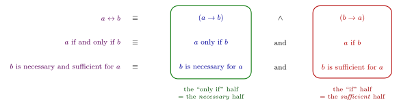
Figure 166: The biconditional decomposed three ways, with each half in its own ringed column. Reading down the left column: a → b, ‘a only if b’, ‘b is necessary for a’ are three names for the same half. Reading down the right: b → a, ‘a if b’, ‘b is sufficient for a’. The whole necessary/sufficient vocabulary is just this correspondence — ‘only if’ is the necessary half, ‘if’ is the sufficient half.
Negating a conditional
\[\sim(p \to q) \;\equiv\; \sim(\sim p \lor q) \;\equiv\; p \land \sim q\]
by the definition of \(\to\), then De Morgan’s law, then the double negative law.
The negation of a conditional is not a conditional — it’s an and. “If it rains, the match is cancelled” is negated by “it rains and the match is not cancelled”, not by “if it rains, the match is not cancelled”.
The classic error is to answer \(\sim p \to \sim q\) (that’s the inverse) or \(q \to p\) (the converse). Neither is the negation, and neither is even equivalent to the original — see Figure 165 above.
Worked: \(\sim(p \to q) \not\equiv \sim p \to \sim q\). Let \(p\) be true and \(q\) be true. Then \(p \to q\) is true, so \(\sim(p \to q)\) is false. But \(\sim p \to \sim q\) is \(\mathrm{F} \to \mathrm{F}\), which is true. The two differ on this row, so they are not equivalent.
Sanity check on the shapes: \(\sim(p \to q)\) is a conjunction and is true on exactly one of the four rows; \(\sim p \to \sim q\) is a conditional and is true on three. They could hardly be equivalent.
Order of operations
- \(\sim\)
- \(\land, \lor\) (equal)
- \(\to, \leftrightarrow\) (equal)
Within a tier, work left to right if no parentheses are given. So \(p \to \sim q \lor r\) means \(p \to \big((\sim q) \lor r\big)\) — but parenthesise explicitly rather than relying on the tie-breaking rule.
Notation, not to be blurred: the biconditional \(\leftrightarrow\) is a connective used to combine statements (like \(+\), \(-\), \(\times\), \(\div\) with numbers). Logical equivalence \(\equiv\) is used when comparing two statements (like \(=\) with numbers). \(a \leftrightarrow b\) is a statement; \(a \equiv b\) is a claim about two statements.
See also
- logical-connectives
- logical-equivalence-laws
- sets-and-set-notation — vacuous truth doing real work, in \(\emptyset \subseteq A\)
- 2026-07-30-conditional-statements — Lecture 3
- practice-problems — §3 Conditional Statements, with full worked solutions
Countable and Uncountable Sets
Which infinite sets are the same size as \(\mathbb{Z}^{+}\), and which are strictly bigger. A set is countable when its elements can be listed, and uncountable when no list can contain them all. Sizes are compared with bijections and injections, as set out in [cardinality]. The lectures are 2026-09-14-cardinalities (the listings) and 2026-09-15-countable-and-uncountable-sets (the definitions and the uncountable sets).
The definitions
A set \(X\) is finite if and only if \(X = \emptyset\) or \(|X| = |\{1,2,\dots,n\}|\) for some \(n \in \mathbb{Z}^{+}\).
A set is infinite if and only if it is not finite.
A set \(X\) is countable if and only if it is finite or \(|X| = |\mathbb{Z}^{+}|\).
A set \(X\) is uncountable if and only if it is not countable.
A set \(X\) is countably infinite if and only if it is countable and infinite.
Every set falls in exactly one of three classes, and “countable” and “infinite” each cover two of them:
| finite | countably infinite | uncountable | |
|---|---|---|---|
| countable? | yes | yes | no |
| infinite? | no | yes | yes |
| \(\lvert X\rvert\) | \(0\) or \(n\) | \(\lvert\mathbb{Z}^{+}\rvert\) | \(> \lvert\mathbb{Z}^{+}\rvert\) |
| examples | \(\emptyset\), \(\{1, \dots, n\}\), \(\{0,1\}\) | \(\mathbb{Z}^{+}\), \(2\mathbb{Z}\), \(\mathbb{Z}\), \(\mathbb{Q}^{+}\), \(\mathbb{Q}\), \(\mathbb{Z} \times \mathbb{Z}\) | \((0,1)\), \(\mathbb{R}\), \(\mathcal{P}(\mathbb{Z}^{+})\) |
The trap is that countable includes finite. “Countable” is not a word for a kind of infinity; “countably infinite” is.
Listing a set
\(X\) is countably infinite if and only if the elements of \(X\) can be written as an infinite list, \(X = \{x_1, x_2, x_3, \dots\}\), where the \(x_i\) are all distinct.
A list is a bijection \(f : \mathbb{Z}^{+} \to X\), \(f(i) = x_i\). “All distinct” is one-to-one, and “every element of \(X\) is somewhere in the list” is onto. To show a set is countably infinite it is enough to describe a list and convince yourself of those two things.
The listings that matter:
| Set | List | Where |
|---|---|---|
| \(2\mathbb{Z}^{+}\) | \(2, 4, 6, 8, \dots\) | 2026-09-14-cardinalities |
| \(\mathbb{Z}\) | \(0, 1, -1, 2, -2, 3, -3, \dots\) | Figure 167; as a formula in cardinality |
| \(\mathbb{Q}^{+}\) | along the anti-diagonals of the \(\frac{a}{b}\) grid, skipping repeats | 2026-09-14-cardinalities |
| \(\mathbb{Z} \times \mathbb{Z}\) | out along a square spiral from \((0,0)\) | 2026-09-14-cardinalities |
| \(\mathbb{Q}\) | along the same spiral, counting only lowest-terms pairs \((a,b)\), with the sign kept in one fixed place (here \(b \geq 1\)) | 2026-09-14-cardinalities |
They are all built the same way. Break the set into finite batches that together cover it, and list the batches one after another. Because each batch is finite, every element comes up after finitely many steps. The batches are \(\{n, -n\}\) for \(\mathbb{Z}\), the anti-diagonals \(a + b = s\) for \(\mathbb{Q}^{+}\), and the square rings for \(\mathbb{Z} \times \mathbb{Z}\).
Figure 167: Two attempts to list \(\mathbb{Z}\); the number above each integer is its place in the list. Top: alternating out from 0 — \(0, 1, -1, 2, -2, \dots\) — reaches every integer after finitely many steps (\(-n\) is in place \(2n+1\)), so it is a list of all of \(\mathbb{Z}\). Bottom: all the positive integers first never finishes them, so 0 and the negatives never get a place, and it is not a list of \(\mathbb{Z}\) at all. A listing must reach every element after finitely many steps; going out in finite batches, here the pairs \({n, -n}\), is how to guarantee it.
Subsets of countable sets
Theorem: Any subset of a countable set is countable.
Corollary: Any set with an uncountable subset is uncountable.
The corollary is the contrapositive of the theorem. For the theorem, take a list of the countable set, keep the members of the subset in the order they come up, and cross out the rest. What is left is a list of the subset, finite if only finitely many survive. The key special case:
Every infinite subset of \(\mathbb{Z}^{+}\) has the same cardinality as \(\mathbb{Z}^{+}\).
Proof. Let \(A \subseteq \mathbb{Z}^{+}\) be infinite. Let \(a_1\) be the least element of \(A\), \(a_2\) the least element of \(A - \{a_1\}\), \(a_3\) the least element of \(A - \{a_1, a_2\}\), and so on. Each step is allowed by the well-ordering principle: what is left is a set of positive integers, and it is non-empty because \(A\) is infinite. Define \(f : \mathbb{Z}^{+} \to A\) by \(f(i) = a_i\).
- \(f\) is one-to-one, because \(a_1 < a_2 < a_3 < \cdots\), so different positions hold different numbers.
- \(f\) is onto, because an element \(a \in A\) has fewer than \(a\) elements of \(A\) below it, all positive integers less than \(a\). So \(a\) is the least element left after at most \(a - 1\) steps, and is picked as some \(a_j\).
So \(|\mathbb{Z}^{+}| = |A|\). \(\square\)

Figure 168: An infinite subset of \(\mathbb{Z}^{+}\), the primes, listed by always taking the least element not yet used. The well-ordering principle guarantees a least element at every step, and the list is increasing, so no prime is used twice. No prime is skipped either: a prime \(p\) has only finitely many primes below it, so it is reached after finitely many steps — 13 has five primes below it and is sixth. So \(i \mapsto a_i\) is a bijection from \(\mathbb{Z}^{+}\) to the primes, and the primes, a sparse and irregular subset, are exactly as numerous as the positive integers.
\(A \subseteq \mathbb{Z}^{+}\) is used twice: in the well-ordering step, which needs a least element at every stage, and in the onto step, “fewer than \(a\) elements below it”. The same construction on \(\mathbb{Q}^{+}\) itself breaks at the first of these, because there is no least positive rational, and that is why \(\mathbb{Q}^{+}\) needed the grid.
\(\mathbb{R}\) is uncountable
It is enough to show that the interval \((0,1)\) is uncountable, because \((0,1) \subseteq \mathbb{R}\) and the corollary does the rest.
Theorem. \((0,1)\) is uncountable.
Proof (by contradiction). Suppose \((0,1)\) is countable. It is infinite, so its elements can be written in a list \(r_1, r_2, r_3, \dots\). Write each as a decimal, \[r_n = 0.\,d_{n1}\,d_{n2}\,d_{n3}\,\dots\] Define a number \(d = 0.\,e_1\,e_2\,e_3\,\dots\) digit by digit, from the diagonal digits \(d_{11}, d_{22}, d_{33}, \dots\): \[e_n = \begin{cases} 1 & \text{if } d_{nn} \neq 1, \\ 2 & \text{if } d_{nn} = 1. \end{cases}\] Then \(d \in (0,1)\). For every \(n\), \(d\) differs from \(r_n\) in the \(n\)-th decimal place, so \(d \neq r_n\). So \(d\) is not in the list, a contradiction. Hence \((0,1)\) is uncountable, and so is \(\mathbb{R}\). \(\square\)
This is Cantor’s diagonal argument. It is worked on a concrete table in 2026-09-15-countable-and-uncountable-sets. Three points in it are easy to get wrong:
- It defeats every list, not one list. The proof never uses anything about the particular list. Whatever list is proposed, the diagonal manufactures a number it misses. That is what “no bijection from \(\mathbb{Z}^{+}\) exists” requires.
- Why the digits 1 and 2. Some numbers have two decimal expansions: \(0.1999\ldots = 0.2000\ldots\). If \(d\) could end in all 0s or all 9s, “differs in a digit” might not mean “is a different number”. A decimal made of 1s and 2s has only the one expansion, so it really is different from every \(r_n\).
- The same argument on \(\mathbb{Q}\) fails. The diagonal of a list of rationals produces a real number, and nothing forces it to be rational. So there is no contradiction, and indeed \(\mathbb{Q}\) is countable.
Not only is \(\mathbb{R}\) bigger than \(\mathbb{Z}^{+}\), it is no bigger than the interval inside it: \(|(0,1)| = |\mathbb{R}|\).
Figure 169: Why the open interval \((0,1)\) has as many points as the whole line. Bend \((0,1)\) into a circle resting on the line, so that its two missing endpoints would meet at the top point \(N\), which is left out. A ray from \(N\) through any other point of the circle meets the line exactly once, and every point of the line is hit by exactly one such ray. Points near the top land far out, the bottom point lands at 0, and nothing is left over on either side — a bijection \((0,1) \to \mathbb{R}\).
The irrational numbers are uncountable as well. If they were countable, \(\mathbb{R} = \mathbb{Q} \cup (\mathbb{R} - \mathbb{Q})\) would be a union of two countable sets and so countable (practice-problems, question 3).
The hierarchy
\[|\emptyset| < |\{1,2,\dots,n\}| < |\mathbb{Z}^{+}| = |\mathbb{Z}| = |\mathbb{Q}| < |\mathbb{R}| < |\mathcal{P}(\mathbb{R})|\]
Figure 170: The sizes of sets met in the course, smallest on the left. Countable covers the first three blocks, empty, finite and countably infinite; infinite covers the last two. Within a block the sets have equal size wherever the chain above writes \(=\): every countably infinite set is the size of \(\mathbb{Z}^{+}\). Crossing a boundary is a strict step up, and the step from countably infinite to uncountable is the diagonal argument. The last block is not all one size: \(\mathcal{P}(\mathbb{R})\) is strictly bigger than \(\mathbb{R}\).
Each strict step has a reason:
- \(|\emptyset| < |\{1, \dots, n\}|\). There is an injection from \(\emptyset\) (the empty function), but no function at all from a non-empty set to \(\emptyset\), so no bijection.
- \(|\{1, \dots, n\}| < |\mathbb{Z}^{+}|\). \(\{1, \dots, n\}\) sits inside \(\mathbb{Z}^{+}\), but no bijection exists, since \(\mathbb{Z}^{+}\) is not finite.
- \(|\mathbb{Z}^{+}| < |\mathbb{R}|\). \(\mathbb{Z}^{+} \subseteq \mathbb{R}\) gives \(\leq\), and the diagonal argument rules out \(=\).
- \(|\mathbb{R}| < |\mathcal{P}(\mathbb{R})|\). Stated without proof. Beyond the course: Cantor’s theorem says \(|A| < |\mathcal{P}(A)|\) for every set \(A\), by a diagonal argument on subsets. So the chain never stops: \(\mathcal{P}(\mathcal{P}(\mathbb{R}))\) is bigger again, and there is no largest size.
How to show a set is countable, or uncountable
Countable — any one of:
- It is finite.
- Write down a list, in finite batches, and check that every element appears exactly once.
- Give a bijection with a set already known to be countable, such as \(\mathbb{Z}^{+}\), \(\mathbb{Z}\), \(\mathbb{Q}\) or \(\mathbb{Z} \times \mathbb{Z}\).
- Give an injection into a countable set. The image is a subset of a countable set, so it is countable, and the injection is a bijection onto its image, so the set itself is countable too. With an injection the other way as well, Schröder–Bernstein gives the exact cardinality, as in the proof that \(\mathbb{Z}^{+} \times \mathbb{Z}^{+}\) is countable using \((a,b) \mapsto 3^a 5^b\) (2026-09-15-countable-and-uncountable-sets).
Uncountable — any one of:
- It contains an uncountable subset, such as an interval of \(\mathbb{R}\).
- There is an injection from a known uncountable set into it, for example from \((0,1)\).
- A diagonal argument: assume a list, and build an element the list misses.
Whatever the direction, the argument has to be a proof. Not being able to think of a list does not show that none exists.
What is assessed. The course practice set marks its whole countable-and-uncountable section (§28) “not assessed in MATH1061”, while Lecture 22 marks only the proof that \(\mathbb{R}\) is uncountable and the countability of \(\mathbb{Z}^{+} \times \mathbb{Z}^{+}\) as not assessed. The two disagree, so check with the course.
See also
- [cardinality] — bijections, the \(|X| = |Y|\) template, \(\leq\) by injection, Schröder–Bernstein
- strong-induction-and-the-well-ordering-principle — the principle that lists an infinite subset of \(\mathbb{Z}^{+}\)
- proof-techniques — proof by contradiction, the shape of the diagonal argument
- rational-and-irrational-numbers — \(\mathbb{Q}\) and \(\overline{\mathbb{Q}}\), on either side of the countable line
- 2026-09-14-cardinalities — Lecture 21 · 2026-09-15-countable-and-uncountable-sets — Lecture 22
- practice-problems — §28, with full worked solutions and the computability application
Counting Principles
The rules for counting the outcomes of a process without listing them. The multiplication rule counts outcomes built in steps. The addition rule counts something that splits into cases that cannot happen together. Subtracting from the total counts what you want by counting what you don’t. Applied to putting objects in order they give permutations, \(n!\) arrangements of \(n\) objects, and \(r\)-permutations, the \(\frac{n!}{(n-r)!}\) ordered selections of \(r\) of them. Selections where order does not matter, and the other kinds of selection, are in counting-selections. First met in 2026-10-12-introduction-to-counting.
The multiplication rule
The multiplication rule. Suppose each outcome is built by \(k\) steps carried out one after another, and that step \(i\) can always be done in \(n_i\) ways, whatever was chosen at the earlier steps. Then the number of outcomes is \[n_1 \times n_2 \times \cdots \times n_k.\]
Each outcome needs exactly one choice at every step, which is why the counts multiply. If step 1 has \(n_1\) options and each of them can be followed by \(n_2\) options at step 2, there are \(n_1\) groups of \(n_2\), which is \(n_1 \times n_2\) two-step beginnings.
“Whatever was chosen at the earlier steps” is the condition to check. It is the number of options that must not depend on earlier choices. The options themselves may change. Arranging \(1, 2, 3, 4, 5\): if 3 goes first, the second position can take 1, 2, 4 or 5, and if 1 goes first it can take 2, 3, 4 or 5. Those are different sets of options, but there are four of them either way, so the rule applies and gives \(5 \times 4 \times 3 \times 2 \times 1 = 120\). When the number of options does change, split into cases first (below).
With two steps, one choice from a set \(A\) and one from a set \(B\), the outcomes are the ordered pairs of \(A \times B\), and the rule is the familiar \(|A \times B| = |A| \times |B|\) (sets-and-set-notation). Choosing one odd and one even number from \(1, \dots, 9\) is \(|D \times E| = 5 \times 4 = 20\), where \(D\) is the odd numbers and \(E\) the even ones. The order the two numbers are picked in does not matter there, but each choice still matches exactly one pair (odd, even), so the count is right (2026-10-12-introduction-to-counting).
Possibility trees
A possibility tree draws a stepwise process. Each level is a step, each branch is one option at that step, and each path from the start to a leaf is one complete outcome. Counting outcomes is counting leaves.
Figure 171: The possibility tree for arranging \({1, 2, 3}\), built one position at a time. Every node at the first level has 2 branches and every node at the second has 1, whichever numbers were used. Because each level splits evenly, the number of leaves is the product of the branch counts, \(3 \times 2 \times 1 = 6\), one for each permutation. If the branch counts at a level differed, the leaves would have to be added up branch by branch.
A tree is worth drawing for a small case even when it is too big to finish, because it shows whether every node at a level has the same number of branches. If it does, multiply. If it doesn’t, as for a permutation of \(\{1, \dots, 7\}\) that starts with a prime followed by an odd number, the leaves have to be added branch by branch (2026-10-12-introduction-to-counting).
Worked: casting two roles
From practice-problems, Q1. Six people audition for Romeo, and eight other people audition for Juliet. How many ways can the lead couple be cast?
Step 1, choose Romeo: 6 ways. Step 2, choose Juliet: 8 ways, whoever was cast as Romeo, because nobody is in both groups. So there are \(6 \times 8 = 48\) ways. If the same person could audition for both roles, step 2’s count would depend on step 1 and the rule could not be used as it stands.
The addition rule
The addition rule. If a finite set \(A\) is the union of mutually disjoint subsets \(A_1, A_2, \dots, A_k\), then \[|A| = |A_1| + |A_2| + \cdots + |A_k|.\]
In counting terms: when every outcome falls into exactly one of several cases, count each case and add. “Mutually disjoint” is the condition of a partition (equivalence-classes-and-partitions): no outcome is in two cases. “Union is \(A\)” means no outcome is left out.
- One number from \(\{1, \dots, 8\}\) that is prime or composite. The primes \(\{2, 3, 5, 7\}\) and the composites \(\{4, 6, 8\}\) are disjoint, because no number is both, so there are \(4 + 3 = 7\).
- Number plates of four, five or six symbols. Every plate has exactly one length, so the counts for the three lengths add (2026-10-12-introduction-to-counting).
- The symbols themselves. 26 letters and 10 digits make \(26 + 10 = 36\) symbols, since no symbol is both.
The cases must not overlap. Count the permutations of \(\{1, \dots, 60\}\) with at least one even number in the first two positions as “first is even” plus “second is even”, and the permutations whose first two numbers are both even are counted twice.
When the sets do overlap, the sum can be corrected rather than abandoned. Adding \(|A|\) and \(|B|\) counts each element of \(A \cap B\) twice, so subtracting it once gives
\[|A \cup B| = |A| + |B| - |A \cap B|,\]
which is the addition rule when \(A \cap B = \emptyset\). For the permutations, in multiples of \(58!\), that is \(1770 + 1770 - 870 = 2670\), the right answer. This is inclusion/exclusion, which extends to three or more sets in inclusion-exclusion.
Figure 172: Why the addition rule needs disjoint cases. Each cell counts the permutations of \({1, \dots, 60}\) whose first two numbers have the given parities, as a multiple of \(58!\). The blue band, first number even, and the orange band, second number even, overlap in the cell EE. Adding the two bands counts EE twice and gets \(3540\), every permutation, although the 870 in OO have no even number in front. Disjoint cases, EE, EO and OE, give the right answer, \(2670\).
When to add and when to multiply
| Multiply | Add | |
|---|---|---|
| Shape | One outcome is built in steps, and every outcome makes one choice at every step. | The outcomes split into cases, and every outcome is in exactly one case. |
| Signals | “followed by”, “then”, “one from each”, positions in an arrangement | an “or” between alternatives that exclude each other; “of length 4, 5 or 6” |
| Check | Is the number of options at each step the same whatever came before? | Do the cases overlap? Do they cover everything? |
| Example | one odd and one even from \(1, \dots, 9\): \(5 \times 4 = 20\) | one number from \(\{1, \dots, 8\}\) that is prime or composite: \(4 + 3 = 7\) |
Most problems use both: multiply within each case, add across the cases. The plates with exactly one digit are an example. Within a length, choose the digit’s position, then the digit, then the letters, and multiply. Across the three lengths, add.
Splitting into cases
The multiplication rule fails when the number of options at a step depends on what was chosen earlier. The fix is to split on that earlier choice, so that inside each case the counts are fixed.
- Find the step whose count varies, and the earlier choice it depends on.
- Split the outcomes into cases according to that choice. The cases must be disjoint and cover everything.
- Apply the multiplication rule inside each case.
- Add the cases.
Worked: a prime followed by an odd number. Permutations of \(\{1, \dots, 7\}\). The primes are \(2, 3, 5, 7\) and the odd numbers \(1, 3, 5, 7\). The number of odd numbers left for position 2 depends on whether the prime in position 1 was odd.
- First number 2: \(1 \times 4 \times 5!\), since all four odd numbers remain.
- First number 3, 5 or 7: \(3 \times 3 \times 5!\), since the first number used up an odd number.
Total \((4 + 9) \times 5! = 1560\). Multiplying straight through, \(4 \times 4 \times 5! = 1920\), overcounts.
Worked: an even number followed by a multiple of 3. Permutations of \(\{1, \dots, 60\}\). There are 30 even numbers and 20 multiples of 3, and 10 of the even numbers, the multiples of 6, are also multiples of 3.
- First number a multiple of 6: \(10 \times 19 \times 58!\), since it used up a multiple of 3.
- First number even but not a multiple of 3: \(20 \times 20 \times 58!\).
Total \((190 + 400) \times 58! = 590 \times 58!\) (2026-10-12-introduction-to-counting).
In both, the split comes from an overlap. A first choice that also belongs to the set the second choice is drawn from uses up one of its options, so it goes in one case, and a first choice outside that set goes in the other.
Counting the complement
If \(A\) is a finite set and \(B \subseteq A\), then \[|A - B| = |A| - |B|.\]
This is the addition rule turned round. \(A\) is the union of the disjoint sets \(B\) and \(A - B\), so \(|A| = |B| + |A - B|\). It is sometimes called the difference rule.
To count the outcomes with some property, count all outcomes and subtract those without it. It pays off whenever the unwanted outcomes are simpler than the wanted ones, which is typical of “at least one”: the opposite of “at least one” is “none”, a single case.
- Prime or composite from \(\{1, \dots, 8\}\). Only 1 is neither: \(|X - \{1\}| = 8 - 1 = 7\).
- At least one even number in the first two positions of a permutation of \(\{1, \dots, 60\}\). The opposite is “both odd”: \(60! - 30 \times 29 \times 58! = 2670 \times 58!\). Counting EE, EO and OE separately gives the same, with three cases instead of one.
- Number plates with at least one repeated symbol. The opposite is “no repeats”, so subtract the plates with no repeats from all plates: \(2\,238\,928\,128 - 1\,449\,063\,000 = 789\,865\,128\).
Subtract inside the same universe. \(B\) has to be a subset of \(A\), counted under the same conditions. For the plates, both counts use lengths 4, 5 and 6 and the same 36 symbols. Subtracting the no-repeat four-symbol plates from all plates of every length would be meaningless.
Permutations
A permutation of a set of objects is an arrangement of the objects into an order.
Theorem. The number of permutations of a set of \(n\) distinct objects is \[n \times (n-1) \times (n-2) \times \cdots \times 2 \times 1 = n!.\]
Why. Fill the positions in turn. The first can hold any of the \(n\) objects. Whatever went there, \(n - 1\) objects remain for the second, then \(n - 2\) for the third, and so on until 1 object remains for the last position. Every step’s count is independent of what was chosen, so the multiplication rule gives \(n!\).
\(n!\) is “\(n\) factorial”, also read “\(n\) bang”:
\[n! = \prod_{i=1}^{n} i \quad\text{for } n \in \mathbb{Z}^{+}, \qquad 0! = 1.\]
\(0! = 1\) is a definition, and it is the one that makes \(n! = n \times (n-1)!\) true at \(n = 1\) (recursive-definitions). The values grow faster than any power: \(5! = 120\), \(6! = 720\), \(10! = 3\,628\,800\), and \(58!\) has 79 digits. Answers to permutation problems are usually left in factorial form for that reason.
| \(n\) | 0 | 1 | 2 | 3 | 4 | 5 | 6 | 7 | 8 |
|---|---|---|---|---|---|---|---|---|---|
| \(n!\) | 1 | 1 | 2 | 6 | 24 | 120 | 720 | 5040 | 40320 |
A bijection \(f\) from \(\{1, \dots, n\}\) to itself is the same thing as the arrangement \(f(1), f(2), \dots, f(n)\), so the symmetric group \(S_n\) has \(n!\) elements (symmetric-group).
Restricted positions: fill them first
When some positions have conditions on them and the rest are free, choose for the restricted positions first. Each later position then has one fewer object than the last, whatever was chosen, and the \(n - k\) free positions are an arrangement of the \(n - k\) objects left: \((n - k)!\) ways.
| Permutations of | that | Count |
|---|---|---|
| \(\{1, \dots, 5\}\) | start with an even number | \(2 \times 4! = 48\) |
| \(\{1, \dots, 7\}\) | start with a prime | \(4 \times 6! = 2880\) |
| \(\{1, \dots, 7\}\) | start with a prime followed by a composite | \(4 \times 2 \times 5! = 960\) |
| \(\{1, \dots, 15\}\) | start with an odd number | \(8 \times 14!\) |
The last line is Q3(a) of practice-problems: \(\{1, \dots, 15\}\) has 8 odd numbers.
Why the restricted position goes first. Filling a free position first makes the count for the restricted one depend on what was used. In “starts with an even number”, if position 2 were filled first, position 1 would have 2 options or only 1, depending on whether position 2 took an even number. Filling position 1 first keeps every count fixed. The second row of the table, \(4 \times 6!\), also shows the most common slip: \(4 \times 6\) forgets that the remaining positions have to be filled too.
\(r\)-permutations
An \(r\)-permutation of a set of \(n\) elements is an ordered selection of \(r\) of the elements, with no element used more than once.
The number of \(r\)-permutations of a set of \(n\) elements, for \(0 \leq r \leq n\), is \[n \times (n-1) \times \cdots \times (n - r + 1) = \frac{n!}{(n-r)!}.\]
Why. It is the permutation count stopped after \(r\) positions. The first position has \(n\) options, the second \(n - 1\), and the \(r\)th has \(n - r + 1\), so there are \(r\) factors. Multiplying top and bottom by the missing factors \((n - r) \times \cdots \times 1 = (n - r)!\) gives the fraction. With \(r = n\) it is \(\frac{n!}{0!} = n!\), the permutations of the whole set, which is one place \(0! = 1\) is needed.
If repetition is allowed, every position has all \(n\) options and the count is \(n^r\). Which of the two applies is the first thing to settle.
Worked: a four-symbol plate. The symbols are the 26 letters and 10 digits, 36 in all.
Figure 173: A four-symbol plate filled one position at a time, from 36 symbols. With repetition allowed, every position has all 36 symbols available, giving \(36^4\). Without repetition, each symbol placed is unavailable afterwards, so each position has one option fewer than the one before. That is a 4-permutation of the 36 symbols, \(36 \times 35 \times 34 \times 33 = \frac{36!}{32!}\).
Over all three lengths these give \(36^4 + 36^5 + 36^6\) plates with repetition and \(\frac{36!}{32!} + \frac{36!}{31!} + \frac{36!}{30!}\) without (2026-10-12-introduction-to-counting). Unordered selections, where only which elements are chosen matters, are counted in counting-selections.
Common mistakes
- Adding steps, or multiplying cases. One prime and one composite is \(4 \times 3 = 12\). One number that is prime or composite is \(4 + 3 = 7\). Getting these the wrong way round gives 7 and 12, swapped.
- Multiplying when a count depends on an earlier choice. “A prime followed by an odd number” is not \(4 \times 4 \times 5!\). After an odd prime only three odd numbers are left. Split into cases.
- Treating an unordered choice as ordered. Choosing one odd and one even number from \(1, \dots, 9\) is 20 ways. Counting “first pick, second pick” gives \(5 \times 4 + 4 \times 5 = 40\), each pair twice.
- Cases that overlap or leave something out. “First is even” plus “second is even” counts the EE permutations twice. Check that each outcome is in exactly one case.
- Forgetting the free positions. Permutations of \(\{1, \dots, 7\}\) starting with a prime are \(4 \times 6!\), not \(4 \times 6\). The other six positions still have to be arranged.
- Mixing up \(n^r\) and \(\frac{n!}{(n-r)!}\). The first allows repeats, the second doesn’t. Read the question for which.
- Subtracting across different universes. The complement has to be counted under the same conditions as the total.
- Counting 1 as a prime or a composite. It is neither, and several of the questions above turn on it.
See also
- 2026-10-12-introduction-to-counting — Lecture 29, with every question worked in full
- counting-selections — ordered and unordered selections, with and without repeats, and more on restrictions
- inclusion-exclusion — counting a union of sets that overlap, where the addition rule does not apply
- probability — the difference rule divided through: \(P(E) = 1 - P(E^c)\)
- pigeonhole-principle — counting pigeons and holes to prove that two must share a hole
- sets-and-set-notation — \(|A \times B| = |A| \times |B|\), the two-step multiplication rule
- equivalence-classes-and-partitions — mutually disjoint sets, the condition in the addition rule
- cardinality — finite sets matched by a bijection have the same size, which is what counting by correspondence relies on
- recursive-definitions — \(n!\) defined recursively, with \(0! = 1\)
- symmetric-group — the \(n!\) bijections of \(\{1, \dots, n\}\)
- practice-problems — §37, with full worked solutions
Counting Selections
Choosing \(r\) objects from a pool of \(n\) can be counted four ways, depending on two questions: does the order of the choices matter, and can the same object be chosen more than once? Each pair of answers has its own formula. This note collects the four, how to tell which one a problem needs, and the standard ways of handling a restriction: forcing part of the selection, splitting the pool into categories, and counting “at least” through the complement. It ends with arrangements of a word that has repeated letters, which are counted by choosing positions. The rules all of this is built from, the multiplication, addition and difference rules, and permutations, are in counting-principles. First met in 2026-10-13-counting-selections.
The two questions
A selection of \(r\) objects from \(n\) is a choice of \(r\) objects, made one after another, from a set of \(n\) distinct objects. Before counting, settle two things.
- Ordered or unordered? In an ordered selection, the same objects chosen in a different order make a different selection: the password cat is not the password cta. In an unordered selection only which objects are chosen counts: the subset \(\{1, 2, 3\}\) is the subset \(\{3, 1, 2\}\). The test is to swap two of the chosen objects. If that changes the outcome, the selection is ordered.
- With or without repeats? With repeats, an object that has been chosen can be chosen again, as a letter can appear twice in a password. Without repeats, each object is used at most once, as each runner finishes a race in one place only.
| without repeats | with repeats | |
|---|---|---|
| ordered | \(\dfrac{n!}{(n-r)!} = n(n-1)\cdots(n-r+1)\) | \(n^r\) |
| unordered | \(\dbinom{n}{r} = \dfrac{n!}{r!\,(n-r)!}\) | \(\dbinom{n+r-1}{r}\) (extension) |
Figure 174: How the four cases are related, with the count for \(n = 10\) and \(r = 3\) in each. Moving right allows an object to be chosen again, which adds the selections that use some object more than once: \(1000 - 720 = 280\) ordered ones and \(220 - 120 = 100\) unordered ones. Moving down forgets the order. Without repeats, each subset was counted once for each of its \(3! = 6\) orders, so the count divides by \(3!\). With repeats that fails, because a selection with a repeated object has fewer orders: 1, 1, 2 has only 3. There \(1000 \div 6\) is not even a whole number. The bottom-right case is extension material.
Ordered, without repeats
There are \(n\) choices for the first object and \(n - 1\) for the second, because the first cannot be used again. Each choice has one fewer option than the one before, and the \(r\)th has \(n - r + 1\). By the multiplication rule (counting-principles) the number of ordered selections without repeats is
\[n(n-1)(n-2)\cdots(n-r+1) = \frac{n!}{(n-r)!}.\]
The product has exactly \(r\) factors. The fraction is the same number written another way: \(n! = n(n-1)\cdots 1\), and dividing by \((n-r)!\) cancels every factor from \(n - r\) down to 1, leaving the top \(r\). For example \(36 \cdot 35 \cdot 34 \cdot 33 = \frac{36!}{32!} = \frac{36!}{(36-4)!}\). These are the \(r\)-permutations of counting-principles, and with \(r = n\) they are the \(n!\) arrangements of all \(n\) objects.
Example. First, second and third place in a race of 10 people: \(10 \cdot 9 \cdot 8 = 720\).
Compute with the product, which never needs a large factorial. The fraction is the compact form for writing the answer down.
Ordered, with repeats
Every one of the \(r\) choices has all \(n\) objects available, so there are
\[n \cdot n \cdots n = n^r\]
ordered selections with repeats. Example. 3-digit passwords: \(10^3 = 1000\), the strings 000 to 999.
The base is the number of objects to choose from and the exponent is the number of choices made. An 8-letter password from a 26-letter alphabet has \(26^8\) possibilities, not \(8^{26}\).
Unordered, without repeats: \(n\) choose \(r\)
An unordered selection without repeats is a subset.
The number of \(r\)-element subsets of an \(n\)-element set is written \(\dbinom{n}{r}\), read “\(n\) choose \(r\)”, and also written \(C(n, r)\): \[\binom{n}{r} = \frac{n!}{r!\,(n-r)!} = \frac{n(n-1)\cdots(n-r+1)}{r(r-1)\cdots 1}.\]
Why divide by \(r!\). Count the ordered selections first: \(n(n-1)\cdots(n-r+1)\). Every \(r\)-element subset appears among them \(r!\) times, once for each order its \(r\) elements can be listed in. So the number of ordered selections is \(r!\) times the number of subsets. For 3 objects from \(\{1, 2, 3, 4\}\) there are \(4 \cdot 3 \cdot 2 = 24\) ordered selections, each subset accounts for \(3! = 6\) of them, and \(\binom43 = \frac{24}{6} = 4\). It is drawn in 2026-10-13-counting-selections.
How to calculate it. Use the second form: \(r\) factors counting down from \(n\) on top, \(r\) factors counting down from \(r\) underneath, and cancel before multiplying.
\[\binom{6}{3} = \frac{6 \cdot 5 \cdot 4}{3 \cdot 2 \cdot 1} = 20, \qquad \binom{10}{3} = \frac{10 \cdot 9 \cdot 8}{3 \cdot 2 \cdot 1} = 120, \qquad \binom{21}{7} = \frac{21 \cdot 20 \cdot 19 \cdot 18 \cdot 17 \cdot 16 \cdot 15}{7 \cdot 6 \cdot 5 \cdot 4 \cdot 3 \cdot 2 \cdot 1} = 116\,280.\]
The answer is always a whole number, because it counts something. A fraction left over means a slip.
Three facts worth knowing.
- \(\binom{n}{r} = \binom{n}{n-r}\). Choosing the \(r\) objects to take is the same as choosing the \(n - r\) to leave behind: each \(r\)-element subset pairs off with its complement, the \(n - r\) elements not in it. So \(\binom{10}{7} = \binom{10}{3} = 120\), and \(\binom{11}{7} = \binom{11}{4} = \frac{11 \cdot 10 \cdot 9 \cdot 8}{4 \cdot 3 \cdot 2 \cdot 1} = 330\). Use whichever has the smaller bottom number. The pairing is drawn in binomial-coefficients, along with the other identities binomial coefficients satisfy.
- \(\binom{n}{n} = \binom{n}{0} = 1\), using \(0! = 1\). For instance \(\binom{2}{2} = \frac{2!}{2!\,0!} = 1\): there is one way to take everything.
- \(\binom{n}{1} = n\).
Unordered, with repeats
Extension material: not assessable in MATH1061. It is Section 9.6 of Epp, and it is covered in MATH2302.
The number of unordered selections of \(r\) objects from \(n\) with repeats allowed is
\[\binom{n+r-1}{r} = \frac{n(n+1)\cdots(n+r-1)}{r(r-1)\cdots 1}.\]
The top now counts up from \(n\), still for \(r\) factors.
Why: stars and bars. Choose 7 candies from 4 colours, red, blue, yellow and pink, where candies of the same colour are identical and a colour can be taken any number of times, including not at all. A selection is settled by how many of each colour are taken. Write an X for each candy, colour by colour, with a bar \(|\) between one colour and the next. Four colours need three bars. Two red, one blue, four yellow and no pink is
\[\mathrm{XX}\,|\,\mathrm{X}\,|\,\mathrm{XXXX}\,|\]
Every string of 7 X’s and 3 bars describes exactly one selection, and every selection gives exactly one such string. So the selections can be counted as strings: 10 positions, of which 3 are bars, and \(\binom{10}{3} = 120\) ways to choose them. In general there are \(r\) X’s and \(n - 1\) bars, \(n + r - 1\) positions in all, and the selection is fixed by which \(r\) of them hold X’s.
Figure 175: Choosing 7 candies from 4 colours, written as strings of 7 X’s and 3 bars. The bars cut the string into four stretches, and the stretches, from left to right, are the red, blue, yellow and pink candies. Top: two red, one blue, four yellow and no pink, so the last stretch is empty. Bottom: two red, two blue, one yellow and two pink. A selection is decided by which 3 of the 10 positions hold the bars, so there are \(\binom{10}{3} = 120\) selections.
Example. Choosing 3 chocolate bars when there are 10 kinds: 3 X’s and 9 bars, so
\[\binom{12}{3} = \frac{12 \cdot 11 \cdot 10}{3 \cdot 2 \cdot 1} = \frac{10 \cdot 11 \cdot 12}{3 \cdot 2 \cdot 1} = 220.\]
Why not \(n^r / r!\)? Dividing by \(r!\) works only when every selection has \(r!\) different orderings, and a selection with a repeat has fewer: \(\{1, 1\}\) has one ordering, not two. For 2 objects from \(\{1, 2, 3, 4\}\), \(4^2 / 2! = 8\), but the true count is \(\binom{5}{2} = 10\).
Which case?
The same \(n = 10\), \(r = 3\) in four questions, one for each case:
| Question | Ordered? | Repeats? | Count |
|---|---|---|---|
| First, second and third in a race of 10 people | yes | no | \(10 \cdot 9 \cdot 8 = 720\) |
| 3-digit passwords | yes | yes | \(10^3 = 1000\) |
| 3-element subsets of \(\{1, 2, \dots, 10\}\) | no | no | \(\binom{10}{3} = 120\) |
| 3 chocolate bars from 10 kinds | no | yes | \(\binom{12}{3} = 220\) |
Wording that usually settles it:
- Subset, committee, hand of cards, “choose 5 of the 11 questions”: unordered, without repeats.
- Password, string, number plate, sequence of digits: ordered, and with repeats unless the problem rules them out.
- First, second and third, or “arrange”: ordered, without repeats.
When the wording is unclear, use the swap test from the two questions and ask whether anything stops an object being picked twice.
Restrictions
A restriction narrows down which selections count. Three moves handle most of them.
Force the restricted part, then fill in the rest. Decide the restricted part first and count the ways it can go, then count the ways to fill whatever is left, and multiply. Ordered selections of 4 from \(\{1, 2, \dots, 10\}\) in which 5 is immediately followed by 6: the block “5 then 6” starts in position 1, 2 or 3 (not 4, where the 6 would have no room), and the two free positions take two of the other 8 numbers in order, \(8 \cdot 7\) ways. So there are \(3 \cdot 8 \cdot 7 = 168\) (2026-10-13-counting-selections). Number plates with exactly one digit go the same way: a \(k\)-symbol plate has \(k\) places for the digit, 10 digits to put there, and 26 letters for each of the other \(k - 1\) places, \(k \cdot 10 \cdot 26^{k-1}\) in all.
Split the pool into categories and choose from each. 5-element subsets of \(\{1, 2, \dots, 11\}\) with 3 even numbers and 2 odd: there are 5 evens and 6 odds, and the two choices are independent, so
\[\binom{5}{3}\binom{6}{2} = 10 \cdot 15 = 150.\]
The binomials are multiplied because every choice of evens goes with every choice of odds.
Split into cases and add. When the count depends on a case, such as the length of a number plate, count each case on its own and add, by the addition rule (counting-principles). The cases must not overlap.
“At least”: count the complement
Counting “at least one” directly means adding up exactly one, exactly two, and so on. The opposite, “none”, is usually a single product. So
\[\#(\text{at least one}) = \#(\text{all}) - \#(\text{none}),\]
which is counting the complement, the difference rule of counting-principles.
| How many … | All | The opposite | At least one |
|---|---|---|---|
| 8-letter passwords contain a vowel? | \(26^8\) | no vowel: \(21^8\) | \(26^8 - 21^8 = 171\,004\,205\,215\) |
| integers from 0 to 9999 contain the digit 5? | \(10^4\) | no 5: \(9^4\) | \(10^4 - 9^4 = 3439\) |
| number plates of 4, 5 or 6 symbols repeat a symbol? | \(36^4 + 36^5 + 36^6\) | no repeat: \(\frac{36!}{32!} + \frac{36!}{31!} + \frac{36!}{30!}\) | \(789\,865\,128\) |
At least two. Take away both “none” and “exactly one”. For 7-element subsets of \(\{1, 2, \dots, 21\}\) with at least two even numbers (10 evens, 11 odds):
\[\binom{21}{7} - \binom{11}{7} - \binom{11}{6}\binom{10}{1} = 116\,280 - 330 - 4620 = 111\,330.\]
“Exactly one even” is itself a categories count: one even from the 10, which is \(\binom{10}{1} = 10\) ways, and six odds from the 11.
Checking with a direct count. The long way gives the same answer and is a good check. Integers from 0 to 9999 with exactly \(k\) fives: choose the \(k\) places for the fives and fill the others from the 9 other digits, \(\binom4k 9^{4-k}\). Then
\[\binom41 9^3 + \binom42 9^2 + \binom43 9 + \binom44 = 2916 + 486 + 36 + 1 = 3439.\]
Fixing one doesn’t work. “Put a vowel in one of the 8 places, then anything anywhere else” gives \(8 \cdot 5 \cdot 26^7 = 321\,272\,407\,040\), which is more than the \(26^8 = 208\,827\,064\,576\) passwords there are. A password with two vowels is counted once for each vowel that could be “the” vowel.
Arrangements of a word with repeated letters
An arrangement uses every letter of the word exactly once, so a word of \(n\) different letters has \(n!\) arrangements. Repeated letters spoil this. Swapping the two B’s of BARBARA gives the same string, so \(7! = 5040\) counts every arrangement more than once.
Count by choosing positions. Place one kind of letter at a time. BARBARA has 7 positions.
- The two B’s go in 2 of the 7 positions: \(\binom72 = 21\) ways. This is a choice of positions, not an ordered selection, because the B’s are identical: once two positions are chosen it makes no difference which B goes in which.
- The three A’s go in 3 of the 5 positions left: \(\binom53 = 10\) ways.
- The two R’s fill the last 2 positions: \(\binom22 = 1\) way.
\[\binom72\binom53\binom22 = 21 \cdot 10 \cdot 1 = 210.\]
Figure 176: Building one arrangement of BARBARA by choosing positions. First the two B’s take 2 of the 7 positions, here 3 and 6, in one of \(\binom72 = 21\) ways. Then the three A’s take 3 of the 5 positions still free, here 1, 4 and 5, in one of \(\binom53 = 10\) ways. The two R’s must take the last two positions, so there is \(\binom22 = 1\) way. Positions already taken are greyed. The result is ARBAABR, one of \(21 \cdot 10 \cdot 1 = 210\) arrangements.
The general formula. Writing the binomials out as factorials, almost everything cancels:
\[\binom72\binom53\binom22 = \frac{7!}{2!\,5!} \cdot \frac{5!}{3!\,2!} \cdot \frac{2!}{2!\,0!} = \frac{7!}{2!\,3!\,2!} = \frac{5040}{24} = 210.\]
In general, a word of \(n\) letters made of \(k\) different letters, appearing \(n_1, n_2, \dots, n_k\) times (so \(n_1 + n_2 + \cdots + n_k = n\)), has
\[\frac{n!}{n_1!\,n_2!\cdots n_k!}\]
distinct arrangements. It also explains the division. Tag the copies so that every letter is different, \(\mathrm{B}_1\mathrm{A}_1\mathrm{R}_1\mathrm{B}_2\mathrm{A}_2\mathrm{R}_2\mathrm{A}_3\), and there are \(7!\) arrangements. Removing the tags merges \(2!\,3!\,2! = 24\) of them into one word, because the tags can be shuffled among the B’s, among the A’s and among the R’s without changing the word.
The order the letters are placed in doesn’t matter. Placing the A’s first gives \(\binom73\binom42\binom22 = 35 \cdot 6 \cdot 1 = 210\) again.
Example: BANANAS. Seven letters: one B, three A’s, two N’s and one S.
\[\frac{7!}{1!\,3!\,2!\,1!} = \frac{5040}{12} = 420.\]
A letter that appears once contributes \(1! = 1\) and can be left out of the denominator.
Restrictions on arrangements use the same moves as before. Letters fixed at the ends are placed first, and the rest of the word is arranged in the positions between. Letters that must sit together are glued into a single tile, which is then arranged along with the other letters. The practice set’s INDOOROOPILLY and WOOLLOONGABBA questions use both moves, and “not next to each other” is counted as all arrangements minus those with the pair glued together.
Common mistakes
- Ordering a subset. \(6 \cdot 5 \cdot 4 = 120\) is the number of ordered selections of 3 from 6. Each 3-element subset is counted \(3! = 6\) times in it, and the number of subsets is \(\binom63 = 20\).
- Dividing by the wrong thing. The divisor for a subset is \(r!\), the number of orders of the \(r\) chosen objects. It is not \(r\), and not 2.
- Swapping \(n\) and \(r\) in \(n^r\). The exponent is the number of choices made: \(26^8\) eight-letter passwords, not \(8^{26}\).
- “Exactly one” without choosing which one. Exactly one even number in a 7-element subset of \(\{1, \dots, 21\}\) is \(\binom{11}{6}\binom{10}{1} = 4620\), not \(\binom{11}{6} = 462\). Leaving out the \(\binom{10}{1}\) gives \(115\,488\) for “at least two evens” in place of the correct \(111\,330\).
- Counting “at least one” by fixing one. It counts selections with several of the wanted objects several times. The complement avoids this.
- A position that cannot be used. A block of two inside four positions has 3 starting places, not 4.
- Numbers of different lengths. To count the integers from 0 to 9999 digit by digit, write every one with four digits, so 7 is 0007. The added zeros never contain a 5, so the count is unchanged, and now every position has 10 choices.
- Treating repeated letters as different. \(7!\) for BARBARA counts each word \(2!\,3!\,2! = 24\) times.
- Using \(n^r / r!\) for unordered selections with repeats. It fails because a selection with a repeat has fewer than \(r!\) orderings.
See also
- counting-principles — the multiplication, addition and difference rules, and permutations, which every formula here is built from
- sets-and-set-notation — subsets, which are what \(\binom{n}{r}\) counts
- binomial-coefficients — Pascal’s formula, the Binomial Theorem, and other identities for \(\binom{n}{r}\), with their combinatorial proofs
- [probability] — probabilities of equally likely outcomes, worked out with these counts
- one-to-one-and-onto-functions — a one-to-one function from an \(r\)-element set to an \(n\)-element set is an ordered selection of images without repeats, so there are \(\frac{n!}{(n-r)!}\) of them
- 2026-10-13-counting-selections — Lecture 30 · 2026-10-12-introduction-to-counting — Lecture 29
- practice-problems — §38, with full worked solutions
Determining Argument Validity — Worked Examples
Worked examples applying the methods from valid-argument-forms — truth table, rules of inference, and the invalidity/counterexample search — on both valid and invalid arguments.
Worked example 1: the pink shirt argument
Consider the argument:
If today is Monday, then I am wearing a pink shirt. Today is Monday. Therefore, I am wearing a pink shirt.
Let \(p\) = “today is Monday” and \(q\) = “I am wearing a pink shirt”. In symbolic form:
\[ \begin{aligned} &1. \quad p \to q \\ &2. \quad p \\ &\therefore \quad q \end{aligned} \]
This is the Modus Ponens form (see valid-argument-forms).
Method 1: checking rows of the truth table
Build a truth table for the premises (\(p \to q\) and \(p\)) and the conclusion (\(q\)). The same table serves all three columns — which column is a premise and which is the conclusion is something you impose on it, not something the table knows, so it is worth labelling the roles before checking anything:
| \(p\) · premise 2 | \(q\) · conclusion | \(p \to q\) · premise 1 |
|---|---|---|
| T | T | T |
| T | F | F |
| F | T | T |
| F | F | T |
An argument is valid iff every row where all the premises are true also has the conclusion true. The premises here are \(p \to q\) and \(p\) — both true only in row 1 (\(p\)=T, \(q\)=T, \(p \to q\)=T). In that row the conclusion \(q\) is also T, and there’s no other row where both premises hold. So the argument is valid.
(To show an argument is invalid by this method, you instead go looking for a row where every premise is T but the conclusion is F. Worked examples 3 and 4 hunt for exactly that combination of truth values, but without building the table — see the invalidity method below.)
Method 2: checking the combined statement is a tautology
Equivalently — and this is the definition — the argument is valid exactly when the single statement
\[(\text{Premise}_1 \land \text{Premise}_2 \land \cdots \land \text{Last Premise}) \to \text{Conclusion}\]
is a tautology. For this argument that statement is \(\big((p \to q) \land p\big) \to q\):
| \(p\) | \(q\) | \(p \to q\) | \(\big((p \to q) \land p\big) \to q\) |
|---|---|---|---|
| T | T | T | T |
| T | F | F | T |
| F | T | T | T |
| F | F | T | T |
Every row is T, so the statement is a tautology — the argument is valid. This is the same conclusion as Method 1, just packaged as one compound formula instead of a row-by-row check across separate premise/conclusion columns. valid-argument-forms has a figure showing why the two readings can never disagree: the rows Method 1 skips are precisely the rows Method 2 gets for free.
A valid argument can still have a false conclusion
This argument is valid regardless of whether \(p\) and \(q\) are actually true today — validity only says “if the premises hold, the conclusion follows”, not that the premises actually do hold. The premise “if today is Monday, then I am wearing a pink shirt” might well be false in reality, and the argument built from it is still valid: the form guarantees the conclusion given the premises, not the truth of the premises themselves.
A false conclusion is fine because validity is a statement about the form. A false premise is fine because it makes the antecedent of \((\text{premises}) \to \text{conclusion}\) false in that row, and a conditional with a false antecedent is true — so that row is T whatever the conclusion does.
Worked example 2: a three-variable argument
Consider the argument:
If wages are raised, buying increases. If there is a depression, buying does not increase. Therefore there is not a depression or wages are not raised.
Let \(w\) = “wages are raised”, \(b\) = “buying increases”, \(d\) = “there is a depression”. (The letters are chosen as mnemonics of the English phrases — the course’s habit whenever a problem starts in words.)
Translating to symbolic form
\[ \begin{aligned} &1. \quad w \to b \\ &2. \quad d \to\; \sim b \\ &\therefore \quad \sim d \lor \sim w \end{aligned} \]
Truth table method
Three variables means \(2^3 = 8\) rows in standard truth table form. The negations \(\sim w\), \(\sim b\), \(\sim d\) are worth building as their own columns first — the premise and conclusion columns are then read straight off them rather than re-derived in your head. In the table below, the ‖ column separates the input block (the variables and their negations) from the compound-form block (the two premises and the conclusion):
| ★ | \(w\) | \(b\) | \(d\) | \(\sim w\) | \(\sim b\) | \(\sim d\) | ‖ | \(w \to b\) | \(d \to \sim b\) | \(\sim d \lor \sim w\) |
|---|---|---|---|---|---|---|---|---|---|---|
| T | T | T | F | F | F | ‖ | T | F | F | |
| ★ | T | T | F | F | F | T | ‖ | T | T | T |
| T | F | T | F | T | F | ‖ | F | T | F | |
| T | F | F | F | T | T | ‖ | F | T | T | |
| F | T | T | T | F | F | ‖ | T | F | T | |
| ★ | F | T | F | T | F | T | ‖ | T | T | T |
| ★ | F | F | T | T | T | F | ‖ | T | T | T |
| ★ | F | F | F | T | T | T | ‖ | T | T | T |
Both premises (\(w \to b\) and \(d \to \sim b\)) are true together in the four starred rows — 2, 6, 7, 8 — and the conclusion \(\sim d \lor \sim w\) is also T in every one of them. There’s no row where both premises hold and the conclusion fails, so the argument is valid. The other four rows are never inspected: each has a false premise, so it cannot break the argument (see valid-argument-forms).
Note that this is not the same as the conclusion being always true — the conclusion is F in rows 1 and 3. Those rows simply have a false premise, so they say nothing about validity.
Rules of inference method
The premises are two conditionals, and the conclusion is a disjunction of two negations. Transitivity is the obvious form to aim at — but the two premises do not chain as they stand, and seeing why is the whole content of this problem:
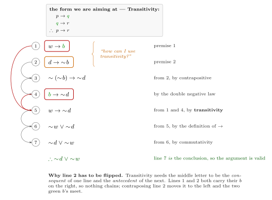
Figure 177: The proof in the course’s three-column layout — line number, statement, justification — with the Transitivity form it aims at shown at the top. The red boxes mark lines 1 and 4, the two that Transitivity chains through the green b where they meet; the orange box marks line 2, the premise that has to be contraposed first. The arrows down the left margin show which earlier lines each step depends on.
Written out in the course’s three-column layout:
| statement | justification | |
|---|---|---|
| 1. | \(w \to b\) | premise 1 |
| 2. | \(d \to \sim b\) | premise 2 |
| 3. | \(\sim(\sim b) \to \sim d\) | from 2, by contrapositive |
| 4. | \(b \to \sim d\) | by the double negative law |
| 5. | \(w \to \sim d\) | from 1 and 4, by Transitivity |
| 6. | \(\sim w \lor \sim d\) | from 5, by the definition of \(\to\) |
| 7. | \(\sim d \lor \sim w\) | from 6, by commutativity |
| \(\therefore\ \sim d \lor \sim w\) | the argument is valid |
Two things to copy from this write-up:
- Write the contrapositive step out before simplifying it. Line 3 is \(\sim(\sim b) \to \sim d\) — the raw contrapositive — and only line 4 cancels the double negative. Collapsing the two makes the justification for line 5 harder to check, because Transitivity needs the forms \(w \to b\) and \(b \to \sim d\) to line up exactly.
- Every line carries a justification. The explanations must be written — the right-hand column is part of the answer, not commentary on it.
Invalidity method, as a third check
Suppose all the premises are true but the conclusion is false.
- Conclusion false \(\Rightarrow\) \(\sim d \lor \sim w\) is false \(\Rightarrow\) \(\sim d\) is false and \(\sim w\) is false \(\Rightarrow\) \(d\) is true and \(w\) is true.
- Premise 1 (\(w \to b\)) is true and \(w\) is true \(\Rightarrow\) \(b\) is true.
- But now \(d\) is true and \(\sim b\) is false, which makes premise 2 (\(d \to \sim b\)) false — contradicting the assumption that all the premises are true.
No consistent assignment exists, so the argument is valid. All three methods — truth table, rules of inference, invalidity search — agree.
Worked example 3: an argument via Conjunction, distribution, and Modus Ponens
Consider the argument (Q1 from the Methods video pre-class questions):
\[ \begin{aligned} &1. \quad p \to q \\ &2. \quad p \lor r \\ &3. \quad p \;\lor \sim r \\ &\therefore \quad q \end{aligned} \]
Rules of inference method
The conclusion \(q\) is the consequent of premise 1, so Modus Ponens finishes the proof the moment \(p\) is available on its own. The whole question is how to manufacture \(p\), and the answer is hiding in the two disjunctive premises.
| statement | justification | |
|---|---|---|
| 1. | \(p \to q\) | given premise |
| 2. | \(p \lor r\) | given premise |
| 3. | \(p \lor \sim r\) | given premise |
| 4. | \((p \lor r) \land (p \lor \sim r)\) | from 2 and 3, by Conjunction |
| 5. | \(p \lor (r \land \sim r)\) | from 4, by the distributive law |
| 6. | \(p \lor \mathbf{c}\) | from 5, by the negation law (\(r \land \sim r \equiv \mathbf{c}\)) |
| 7. | \(p\) | from 6, by the identity law |
| 8. | \(q\) | from 1 and 7, by Modus Ponens |
The trick is spotting that the two premises \(p \lor r\) and \(p \lor \sim r\) share the same left disjunct, so conjoining them and distributing \(p\) back out leaves “\(p\), or a contradiction” — which forces \(p\) to be true regardless of \(r\). The equivalence laws used at lines 5–7 are in logical-equivalence-laws.
Invalidity method, as a check
Suppose all the premises are true but the conclusion is false.
- Conclusion false \(\Rightarrow\) \(q\) is false.
- Premise 1 (\(p \to q\)) is true and \(q\) is false \(\Rightarrow\) \(p\) is false.
- Premise 2 (\(p \lor r\)) is true and \(p\) is false \(\Rightarrow\) \(r\) is true.
- Premise 3 (\(p \lor \sim r\)) is true and \(p\) is false \(\Rightarrow\) \(\sim r\) is true, i.e. \(r\) is false.
\(r\) can’t be both true and false — impossible. No such truth values exist, so the argument is valid, agreeing with the rules-of-inference proof above.
Worked example 4: an invalid argument
Not every argument is valid. Consider (Q2 from the Methods video pre-class questions):
\[ \begin{aligned} &1. \quad p \to q \\ &2. \quad q \to r \\ &3. \quad \sim p \;\lor \sim q \\ &\therefore \quad r \end{aligned} \]
Invalidity method
Suppose all the premises are true but the conclusion is false.
- Conclusion false \(\Rightarrow\) \(r\) is false.
- Premise 2 (\(q \to r\)) is true and \(r\) is false \(\Rightarrow\) \(q\) is false.
- Premise 1 (\(p \to q\)) is true and \(q\) is false \(\Rightarrow\) \(p\) is false.
- Premise 3 (\(\sim p \lor \sim q\)), checked against \(p\) false and \(q\) false: it’s true. No contradiction anywhere.
This gives a consistent assignment — \(p\), \(q\), \(r\) all false — that makes every premise true and the conclusion false:
| \(p\) | \(q\) | \(r\) | \(p \to q\) | \(q \to r\) | \(\sim p \lor \sim q\) | \(r\) |
|---|---|---|---|---|---|---|
| F | F | F | T | T | T | F |
All three premises hold, the conclusion doesn’t — that’s a counterexample, so the argument is invalid.
Note the shape of the last step: once every variable has been forced, premise 3 has to be checked, not used to force anything further. If it had come out false the search would have closed with a contradiction instead, and the argument would have been valid.
How the search ends is the whole verdict
Worked examples 3 and 4 run the same procedure and part company only at the end. Setting them side by side is the clearest statement of what the method actually decides:
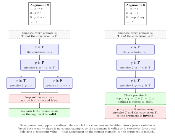
Figure 178: The invalidity search drawn as the cascade of forced values it produces, on the two arguments that end it differently. Assuming the conclusion false and every premise true forces variable after variable; the left-hand search (worked example 3) closes because r is forced both ways, so no counterexample exists and the argument is valid, while the right-hand search (worked example 4) runs to completion with every value consistent, and that assignment is the counterexample.
Because of that, the invalidity search is the method of choice when you don’t yet know the answer: it settles the question either way, and when the argument fails it hands you the counterexample rather than just the news that no proof turned up. A rules-of-inference attempt that stalls tells you nothing.
See also
- valid-argument-forms
- logical-equivalence-laws
- 2026-08-03-valid-and-invalid-arguments — Lecture 4
- practice-problems — §5 Methods for Determining Validity, with full worked solutions
Divisibility & Unique Factorisation
Definition
\[d \mid n \iff d \neq 0 \text{ and } n = dk \text{ for some integer } k\]
Both \(n\) and \(d\) must be integers, and \(d \neq 0\) — this side condition is part of the definition, not an afterthought. Equivalently, \(d \mid n \iff \frac{n}{d} \in \mathbb{Z}\).
All of these say the same thing:
- \(d\) divides \(n\)
- \(d\) is a divisor of \(n\)
- \(d\) is a factor of \(n\)
- \(n\) is a multiple of \(d\)
\(d \nmid n\) means \(d\) does not divide \(n\). Note that \(d \mid n\) is a statement, not a number: \(2 \mid 6\) is true, it is not “\(2\) divided by \(6\)” and it is not \(3\). Likewise \(10 \nmid 5\) is true, since \(\frac{5}{10} \notin \mathbb{Z}\). Being a statement is what makes \(2 \mid x\) a predicate — it acquires a truth value once \(x\) is fixed — so it is exactly the kind of thing a quantifier can be put in front of.
Divisibility inside a quantified statement
Two quantified divisibility statements, both false, both settled by a single counterexample — one counterexample is enough to make a \(\forall\) statement false, though no single example could ever make one true (see quantified-statements on that asymmetry):
| Statement | Verdict | Counterexample |
|---|---|---|
| \(\forall x \in \mathbb{Z}\), if \(2 \mid x\) then \(4 \mid x\) | False | \(x = 2\): \(2 \mid 2\) is true but \(4 \nmid 2\) |
| \(\forall x \in \mathbb{Z}\), if \(6\) is divisible by \(x\), then \(x = 2\) | False | \(x = 3\): \(3 \in \mathbb{Z}\) and \(3 \mid 6\), but \(3 \neq 2\) |
A counterexample to a universal conditional has to make the hypothesis true and the conclusion false — that is what \(\sim(p \to q) \equiv p \land \sim q\) says. An \(x\) that fails the hypothesis proves nothing.
The second statement becomes true once the conclusion lists every divisor:
\[\forall x \in \mathbb{Z}, \text{ if } 6 \text{ is divisible by } x, \text{ then } x = \pm 1 \text{ or } \pm 2 \text{ or } \pm 3 \text{ or } \pm 6.\]
The \(\pm\) is not optional. The reason is in the definition: it asks only for \(n = dk\) with \(k \in \mathbb{Z}\), and \(k\) may be negative, so divisors over \(\mathbb{Z}\) always come in \(\pm\) pairs — if \(n = dk\) then \(n = (-d)(-k)\), so \(d \mid n\) exactly when \((-d) \mid n\). A divisor list that quietly restricts itself to \(\mathbb{Z}^+\) is answering a question about a different domain.
Proving and disproving divisibility statements
The pattern for a direct proof: unfold \(d \mid n\) into \(n = dk\), do algebra, then re-fold into the definition by exhibiting the integer witness.
\(\forall a, b, c \in \mathbb{Z}\), if \(c \mid a\) then \(c \mid ab\).
Let \(a, b, c \in \mathbb{Z}\) and suppose \(c \mid a\). Then \(\exists k \in \mathbb{Z}\) such that \(a = ck\). Multiplying both sides by \(b\): \(ab = ckb = c(kb)\). Since \(k, b \in \mathbb{Z}\) we have \(kb \in \mathbb{Z}\). Thus \(c \mid ab\). \(\square\)
\(\forall m \in \mathbb{Z}\), \(6m(2m + 10m^2)\) is divisible by 4.
Let \(m \in \mathbb{Z}\). Then \(6m(2m + 10m^2) = 2(3m) \cdot 2(m + 5m^2) = 4 \big(3m(m + 5m^2)\big)\). Since \(m \in \mathbb{Z}\), \(3m(m + 5m^2) \in \mathbb{Z}\). Thus \(4 \mid 6m(2m + 10m^2)\). \(\square\)
\(\forall a, b, c \in \mathbb{Z}\), if \(a \mid (b + c)\) then \(a \mid b\) or \(a \mid c\) — false. Counterexample \(a = 3, b = 4, c = 2\): \(a \mid (b+c)\) since \(3 \mid 6\), but \(3 \nmid 4\) and \(3 \nmid 2\).
\(\forall a, b, m \in \mathbb{Z}\), if \(m \mid (a+b)\) then \(m \mid (a-b)\) — false. A counterexample needs the hypothesis true and the conclusion false:
| \(m \mid (a+b)\) | \(m \mid (a-b)\) | conditional | |
|---|---|---|---|
| \(m=5, a=20, b=10\) | \(5 \mid 30\) T | \(5 \mid 10\) T | T |
| \(m=5, a=21, b=13\) | \(5 \mid 34\) F | \(5 \mid 8\) F | T |
| \(m=5, a=27, b=7\) | \(5 \mid 34\) F | \(5 \mid 20\) T | T |
| \(m=5, a=19, b=-9\) | \(5 \mid 10\) T | \(5 \mid 28\) F | F |
| \(m=5, a=23, b=12\) | \(5 \mid 35\) T | \(5 \mid 11\) F | F |
| \(m=5, a=-10, b=-3\) | \(5 \mid -13\) F | \(5 \mid -7\) F | T |
Only the two rows with hypothesis T and conclusion F are counterexamples.
\(\forall m, n, q \in \mathbb{Z}\), if \(m \mid n\) and \(n \mid q\) then \(m^2 \mid nq\) — true.
Let \(m, n, q\) be non-zero integers with \(m \mid n\) and \(n \mid q\). By definition there exist \(a, b \in \mathbb{Z}\) with \(n = ma\) and \(q = nb\). Then \[nq = (ma)(nb) = ma \cdot (mab) = m^2(a^2b).\] Since \(a^2 b \in \mathbb{Z}\), we conclude \(m^2 \mid nq\). \(\square\)
If \(k\) is even and \(m\) is odd, then \((k+2)^2 - (m-3)^2\) is divisible by 4.
Let \(k = 2a\) and \(m = 2b+1\) for some \(a, b \in \mathbb{Z}\). Then \((k+2)^2 = (2a+2)^2 = 4(a+1)^2\) and \((m-3)^2 = (2b-2)^2 = 4(b-1)^2\), so \[(k+2)^2 - (m-3)^2 = 4\big((a+1)^2 - (b-1)^2\big),\] and \((a+1)^2 - (b-1)^2 \in \mathbb{Z}\). \(\square\)
\(\forall c, d, e \in \mathbb{Z}\), if \(c \mid d\) and \(c \nmid e\), then \(c \nmid (d+e)\).
Proof by contradiction. Suppose there exist integers \(c, d, e\) with \(c \mid d\), \(c \nmid e\) and \(c \mid (d+e)\). Then \(d = cx\) for some \(x \in \mathbb{Z}\), and \(d + e = cy\) for some \(y \in \mathbb{Z}\). Hence \(cx + e = cy\), so \(e = c(y - x)\) with \(y - x \in \mathbb{Z}\) — so \(c \mid e\), a contradiction. \(\square\)
Every integer \(n > 1\) is a product of primes
Proof by contradiction. Suppose the theorem is false. Then there exists an integer \(n > 1\) that is not a product of primes. Choose the smallest such \(n\) — such a smallest one exists by the well-ordering principle. Choosing the smallest is what lets us assume every integer strictly between \(1\) and \(n\) is a product of primes.
Every integer \(n > 1\) is either prime or composite (not both).
Case 1: \(n\) is prime. Then \(n\) is a product of primes (namely itself) — contradiction.
Case 2: \(n\) is composite. Then \(n = rs\) for positive integers \(r, s\) with \(r \neq 1\) and \(s \neq 1\), which forces \(1 < r < n\) and \(1 < s < n\). Because \(n\) was chosen smallest, both \(r\) and \(s\) are products of primes, say \(r = p_1 p_2 \cdots p_k\) and \(s = q_1 q_2 \cdots q_\ell\). Therefore \(n = rs = p_1 \cdots p_k q_1 \cdots q_\ell\) is a product of primes too.
Either way \(n\) is a product of primes, contradicting our choice of \(n\). \(\square\)
Unique Factorisation Theorem
Provided in the exam. This theorem and the Quotient-Remainder Theorem are both stated on the MATH1061/MATH7861 Examination Formula Page, so they can be cited rather than restated from memory — see also logical-equivalence-laws for the rest of what that page carries.
Given any integer \(n > 1\), the standard factored form of \(n\) is \[n = p_1^{e_1} p_2^{e_2} \cdots p_k^{e_k}\] where \(k \in \mathbb{Z}^+\), the \(p_i\) are primes, the \(e_i\) are positive integers, and \(p_1 < p_2 < \cdots < p_k\).
Both the primes and their exponents are unique — this is what makes the factored form a canonical fingerprint of an integer, and it’s the engine behind divisor counting, gcd and lcm (see gcd-lcm-and-euclidean-algorithm).
Counting divisors from the factorisation
Any positive divisor of \(n = p_1^{e_1} \cdots p_k^{e_k}\) has the form \(p_1^{a_1} \cdots p_k^{a_k}\) with \(0 \leq a_i \leq e_i\), so there are
\[(e_1 + 1)(e_2 + 1) \cdots (e_k + 1)\]
positive divisors.
\(6975 = 3^2 \cdot 5^2 \cdot 31\), found by trial division: \(6975 = 3 \cdot 2325 = 3 \cdot 3 \cdot 775 = 3 \cdot 3 \cdot 5 \cdot 155 = 3^2 \cdot 5^2 \cdot 31\). A divisor has \(0\), \(1\) or \(2\) threes; \(0\), \(1\) or \(2\) fives; and \(0\) or \(1\) thirty-ones — so \(3 \cdot 3 \cdot 2 = 18\) positive divisors.
\(27720 = 2^3 \cdot 3^2 \cdot 5 \cdot 7 \cdot 11\).
\(1400 = 2^3 \cdot 5^2 \cdot 7\), worked through:
- \(1400 = 2(700) = 2 \cdot 2(350) = 2 \cdot 2(35)(10) = 2^2 (5 \cdot 7)(2 \cdot 5) = 2^3 \cdot 5^2 \cdot 7^1\) — note the primes are written in increasing order.
- \(1400^2 = (2^3 \cdot 5^2 \cdot 7)^2 = 2^6 \cdot 5^4 \cdot 7^2\) — raising to a power multiplies the exponents.
- \(1400^3 = 1400 \cdot 1400^2 = 2^9 \cdot 5^6 \cdot 7^3\) — multiplying adds the exponents.
- Number of positive divisors of \(1400\): \((3+1)(2+1)(1+1) = 24\).
- Divisors of \(1400\) divisible by \(8\): all factors of the form \(2^3 \cdot 5^* \cdot 7^*\), i.e. \(8, 40, 200, 56, 280, 1400\).
- Smallest \(n\) with \(1400n\) a perfect square: \(1400n = t^2\) needs every exponent even. \(t^2 = 2^3 \cdot 5^2 \cdot 7^1 \cdot n\), and splitting each power in half (bigger halves on the left) gives \(t = 2^2 \cdot 5^1 \cdot 7^1\) against \(2^1 \cdot 5^1 \cdot 7^0 \cdot n\), so \(n = 2 \cdot 7 = 14\).
Primality testing
Lemma: for every integer \(n > 1\), if no integer \(x\) in the range \(1 < x \leq \sqrt{n}\) divides \(n\), then \(n\) is prime.
This is why trial division only has to go as far as \(\sqrt{n}\) — for \(6975\), only up to \(\sqrt{6975} = 83.51\dots\)
Proof by contraposition. The contrapositive is: \(\forall n \in \mathbb{Z}^{\geq 2}\), if \(n\) is not prime, then there exists an integer \(x\) with \(1 < x \leq \sqrt{n}\) such that \(x \mid n\).
Suppose \(n \in \mathbb{Z}^{\geq 2}\) and \(n\) is not prime. Then \(n\) is composite, so by definition \(\exists r, s \in \mathbb{Z}^+\) with \(n = rs\) and \(1 < r < n\) and \(1 < s < n\).
Case 1: \(r = s\). Then \(r = s = \sqrt{n}\).
Case 2: \(r \neq s\). Then one of \(r, s\) is less than \(\sqrt{n}\) and the other greater — if both were greater we’d have \(rs > n\), and if both were less we’d have \(rs < n\).
In either case there is an \(x \in \{r, s\}\) with \(1 < x \leq \sqrt{n}\) and \(x \mid n\). \(\square\)
There are infinitely many primes
Lemma: for any integer \(a\) and any prime \(p\), if \(p \mid a\) then \(p \nmid (a+1)\).
Proof by contradiction. Let \(a \in \mathbb{Z}\), let \(p\) be prime, suppose \(p \mid a\), and assume for a contradiction that \(p \mid (a+1)\). Since \(p \mid a\) there exists \(k \in \mathbb{Z}\) with \(a = pk\); since \(p \mid (a+1)\) there exists \(\ell \in \mathbb{Z}\) with \(a + 1 = p\ell\). So \[1 = (a+1) - a = p\ell - pk = p(\ell - k),\] and \(\ell - k \in \mathbb{Z}\), so \(p \mid 1\). But \(p \geq 2\) for any prime, whereas \(p \mid 1\) forces \(p = \pm 1\) — a contradiction. \(\square\)
Theorem: there are an infinite number of primes.
Proof by contradiction. Suppose the number of primes is finite. Then some prime \(p\) is the largest, and we can list every prime in ascending order: \(2, 3, 5, 7, 11, \dots, p\).
Let \(N = (2 \cdot 3 \cdot 5 \cdot 7 \cdot 11 \cdots p) + 1\).
Then \(N > 1\), so by the Unique Factorisation Theorem \(N\) is a product of primes and hence divisible by some prime \(q\). Because \(q\) is prime it must be one of \(2, 3, 5, 7, 11, \dots, p\).
So \(q\) divides \(2 \cdot 3 \cdot 5 \cdots p\) — that is, \(q \mid (N - 1)\) — and hence by the lemma \(q \nmid \big((2 \cdot 3 \cdot 5 \cdots p) + 1\big) = N\).
So \(q\) divides \(N\) and \(q\) does not divide \(N\): a contradiction. Therefore the original statement is true. \(\square\)
See also
- proof-techniques · modular-arithmetic · gcd-lcm-and-euclidean-algorithm
- partial-order-relations — “divides” as a partial order on \(\mathbb{Z}^{+}\)
- fields — unique factorisation as the reason \(\mathbb{Z}_p\) is a field when \(p\) is prime
- counting-principles — the rule behind counting divisors, one choice of exponent for each prime
- practice-problems — §13 Divisibility, with full worked solutions
Equivalence Classes and Partitions
An equivalence relation sorts its set into groups of mutually related elements, the equivalence classes. The classes cut the set into non-overlapping pieces, a partition, and every partition comes from an equivalence relation in this way. Equivalence relations themselves are in equivalence-relations. First met in 2026-09-21-equivalence-relations, and finished at the start of 2026-09-22-partial-order-relations.
The definition
Let \(\rho\) be an equivalence relation on a set \(S\). For each \(a \in S\), define the equivalence class of \(a\) by \[[a] = \{x \in S : x \mathrel{\rho} a\}\] (the set of elements related to \(a\)).
Three things to read off the definition:
- \([a]\) is a set, a subset of \(S\). It is not an element of \(S\), and it is not a number.
- \(a \in [a]\) always, because \(\rho\) is reflexive. So no class is empty.
- The bracket depends on the relation. \([1]\) means one thing for congruence mod 3 and another for \(x - y \in \mathbb{Q}\). Say which relation is meant.
| Relation | Class | As a set |
|---|---|---|
| \(m \equiv n \pmod 3\) on \(\mathbb{Z}\) | \([1]\) | \(\{\dots, -5, -2, 1, 4, 7, \dots\}\) |
| same parity on \(\mathbb{Z}\) | \([0]\) | \(\mathbb{Z}^{even}\) |
| \(x - y \in \mathbb{Q}\) on \(\mathbb{R}\) | \([1]\) | \(\mathbb{Q}\) |
| \(x - y \in \mathbb{Q}\) on \(\mathbb{R}\) | \([\sqrt2]\) | \(\{y + \sqrt2 : y \in \mathbb{Q}\}\) |
| same part of \(\{\{1,2,3\},\{4,5\},\{6\}\}\) | \([4]\) | \(\{4, 5\}\) |
Describing a class
To find \([a]\), ask which \(x\) are related to \(a\): write down \(x \mathrel{\rho} a\), unfold the definition of \(\rho\), and simplify until it is a plain condition on \(x\).
\([1]\) for \(x \mathrel{\tau} y \leftrightarrow x - y \in \mathbb{Q}\). A real \(y\) is related to 1 exactly when \(1 - y \in \mathbb{Q}\), which happens exactly when \(y \in \mathbb{Q}\). So \([1] = \mathbb{Q}\).
\([\sqrt2]\) for the same relation. \(x \mathrel{\tau} \sqrt2\) means \(x - \sqrt2 = y\) for some \(y \in \mathbb{Q}\), that is, \(x = y + \sqrt2\). So \([\sqrt2] = \{y + \sqrt2 : y \in \mathbb{Q}\}\). It contains \(\sqrt2\), \(1 + \sqrt2\), \(-3 + \sqrt2\), and so on.
\([1]\) for \(m \mathrel{\sigma} n \leftrightarrow 8 \mid (m - n) \text{ or } 8 \mid (m + n)\). \[[1] = \{n \in \mathbb{Z} : 8 \mid (1 - n) \text{ or } 8 \mid (1 + n)\} = \{n \in \mathbb{Z} : n \equiv 1 \text{ or } 7 \pmod 8\}.\] The second alternative says \(n \equiv -1 \pmod 8\), and \(-1 \equiv 7\). All five classes of \(\sigma\) are in 2026-09-22-partial-order-relations.
These three are worked in 2026-09-21-equivalence-relations and 2026-09-22-partial-order-relations. The definition has \(x \mathrel{\rho} a\) and the workings sometimes use \(a \mathrel{\rho} x\). For an equivalence relation the two say the same thing, by symmetry.
When the class is infinite, describe it by a condition, as above. Listing “\(\{\dots, -7, -1, 1, 7, 9, \dots\}\)” is a useful check, but the pattern has to be stated.
One class, many names
For congruence mod 3, \[[0] = [3] = [-6].\] These are three names for one set, \(\{\dots, -6, -3, 0, 3, 6, \dots\}\). The element inside the bracket is a representative of the class, and every element of a class is a representative of it. The rule for when two names give the same class is:
\([a] = [b]\) if and only if \(a \mathrel{\rho} b\).
So to decide whether two classes are equal, test the two representatives against each other. For example, is \([\sqrt2] = [-\sqrt2]\) for \(\tau\)? \(\sqrt2 - (-\sqrt2) = 2\sqrt2 \notin \mathbb{Q}\), so \(\sqrt2 \mathrel{\not\tau} {-\sqrt2}\), and \([\sqrt2] \neq [-\sqrt2]\).
The rule follows from the result in the next section: if \(a \mathrel{\rho} b\) the classes are equal, and if \(a \mathrel{\not\rho} b\) they are disjoint and non-empty, so not equal. By convention the simplest representative is used. For congruence mod \(n\) the usual choice is \([0], [1], \dots, [n-1]\) (integers-modulo-n).
Equal or disjoint
Important result. If \(\rho\) is an equivalence relation on a set \(S\), and \(a, b \in S\), then either \[[a] = [b] \qquad \text{or} \qquad [a] \cap [b] = \emptyset.\] If \(a \mathrel{\rho} b\) the classes are equal. If \(a \mathrel{\not\rho} b\) they are disjoint.
Two classes never partly overlap. The proof uses each of the three properties.
Proof. Let \(\rho\) be an equivalence relation on \(S\) and let \(a, b \in S\).
Case 1: \(a \mathrel{\rho} b\). We show \([a] \subseteq [b]\) and \([b] \subseteq [a]\). Let \(x \in [a]\). Then \(x \mathrel{\rho} a\). Since also \(a \mathrel{\rho} b\), transitivity gives \(x \mathrel{\rho} b\), so \(x \in [b]\). Hence \([a] \subseteq [b]\). By symmetry, \(b \mathrel{\rho} a\), and the same argument with \(a\) and \(b\) exchanged gives \([b] \subseteq [a]\). Hence \([a] = [b]\).
Case 2: \(a \mathrel{\not\rho} b\). Suppose, for a contradiction, that \([a] \cap [b] \neq \emptyset\), and take \(x \in [a] \cap [b]\). Then \(x \mathrel{\rho} a\) and \(x \mathrel{\rho} b\). By symmetry, \(a \mathrel{\rho} x\). By transitivity, \(a \mathrel{\rho} x\) and \(x \mathrel{\rho} b\) give \(a \mathrel{\rho} b\). \((\Rightarrow\Leftarrow)\) Hence \([a] \cap [b] = \emptyset\). \(\square\)
Reflexivity is what puts \(a\) into \([a]\). It gives if \([a] = [b]\) then \(b \in [a]\) in one line: \(b \in [b] = [a]\).
Figure 179: The two things that can happen to two equivalence classes, and the one that cannot. Left: if \(a \mathrel{\rho} b\) then \([a]\) and \([b]\) are the same set. Middle: if \(a\) and \(b\) are not related then the two classes share no element. Right: a partial overlap is impossible. A shared element \(x\) is related to both \(a\) and \(b\); symmetry turns \(x \mathrel{\rho} a\) round into \(a \mathrel{\rho} x\), and transitivity along \(a \to x \to b\) then forces \(a \mathrel{\rho} b\), the dashed arrow, which puts the pair back in the left-hand picture.
Putting the pieces together, for an equivalence relation \(\rho\) these four statements stand or fall together:
\[a \mathrel{\rho} b \qquad\qquad [a] = [b] \qquad\qquad b \in [a] \qquad\qquad [a] \cap [b] \neq \emptyset\]
Partitions
Two sets \(X\) and \(Y\) are disjoint if and only if \(X \cap Y = \emptyset\).
A collection of sets is mutually disjoint if each pair of distinct sets in the collection is disjoint.
A partition of a set \(S\) is a collection of non-empty and mutually disjoint subsets of \(S\) whose union is \(S\). The subsets in a partition are sometimes called parts.
So a collection of subsets of \(S\) is a partition when it passes three checks:
- every part is non-empty;
- the parts are mutually disjoint: no element is in two of them;
- their union is \(S\): no element is left out.
Checks 2 and 3 together say that every element of \(S\) is in exactly one part. The same definition, in Lecture 17’s words and with more worked examples, is in sets-and-set-notation.
Mutually disjoint is about pairs. \(W = \{1,2,3\}\), \(X = \{4,5,6\}\), \(Y = \{6,7,8\}\) are not mutually disjoint, because \(X \cap Y = \{6\}\), even though \(W\) is disjoint from both of the others. More examples are in 2026-09-21-equivalence-relations.
The classes form a partition
The equivalence classes of an equivalence relation on a set \(S\) form a partition of the set \(S\).
The three checks, for the collection of all classes \(\{[a] : a \in S\}\):
- Non-empty. \(a \in [a]\), by reflexivity.
- Mutually disjoint. Two distinct classes are not equal, so by the result above they are disjoint.
- Union is \(S\). Each \(a \in S\) lies in the class \([a]\), and every class is a subset of \(S\).
In the collection each class is counted once, however many names it has. For congruence mod 3 the collection is \(\{[0], [1], [2]\}\), with three members, although \([0] = [3] = [-6] = \cdots\).
| Relation | Number of classes |
|---|---|
| \(m \equiv n \pmod 3\) on \(\mathbb{Z}\) | 3 |
| same parity on \(\mathbb{Z}\) | 2 |
| \(8 \mid (m-n)\) or \(8 \mid (m+n)\) on \(\mathbb{Z}\) | 5 |
| \(x - y \in \mathbb{Q}\) on \(\mathbb{R}\) | infinitely many |
| \(x = y\) on a set \(S\) | one for each element of \(S\) |
From a partition to a relation
Given any partition of a set \(S\), we can define an equivalence relation on \(S\), by defining two elements to be related if and only if they are in the same part of the partition. The parts in a partition form the equivalence classes of the corresponding equivalence relation.
“In the same part” is an equivalence relation. The check is short, and it shows what each condition on a partition is for.
- Reflexive. Let \(x \in S\). The union of the parts is \(S\), so \(x\) is in some part, and it is in the same part as itself.
- Symmetric. If \(x\) and \(y\) are in the same part, then \(y\) and \(x\) are.
- Transitive. Suppose \(x\) and \(y\) are both in a part \(P\), and \(y\) and \(z\) are both in a part \(Q\). Then \(y \in P \cap Q\). The parts are mutually disjoint, so \(P\) and \(Q\) cannot be distinct: \(P = Q\). So \(x\) and \(z\) are in the same part.
Reflexivity uses “the union is \(S\)”, and transitivity uses “mutually disjoint”.
Writing the relation down. For a small set, list the pairs: a part with \(k\) elements gives all \(k^2\) ordered pairs of its elements. The partition \(\{\{1,2,3\},\{4,5\},\{6\}\}\) of \(\{1,\dots,6\}\) gives \(9 + 4 + 1 = 14\) pairs, drawn in 2026-09-21-equivalence-relations. For an infinite set, turn “in the same part” into a condition. For the partition \(\{\mathbb{Z}^{-}, \{0\}, \mathbb{Z}^{+}\}\) of \(\mathbb{Z}\) the condition is
\(a \mathrel{\tau} b \longleftrightarrow a, b\) both positive \(\ \) or \(\ a = b = 0\ \) or \(\ a, b\) both negative
with one alternative for each part (2026-09-22-partial-order-relations).
Two descriptions of one thing
Any partition defines an equivalence relation and any equivalence relation defines a partition.
In short, equivalence relations \(\iff\) partitions. The two constructions undo each other:
- Start with an equivalence relation, take its classes, and relate elements in the same class. That gives back the relation you started with, since \(x \mathrel{\rho} y\) exactly when \([x] = [y]\).
- Start with a partition, relate elements in the same part, and take the classes. That gives back the parts.
So an equivalence relation on \(S\) and a partition of \(S\) carry the same information. A question about one can be answered with the other. To count or describe the equivalence relations on a small set, describe its partitions. To show a collection of sets is a partition, it is enough to recognise it as the classes of an equivalence relation.
Finding the classes of a finite relation
For an equivalence relation given by a list of pairs or an arrow diagram:
- Pick any element \(a\). Its class is \(a\) together with everything joined to \(a\) by an arrow.
- Pick any element not yet in a class, and do the same.
- Stop when every element is in a class.
Step 1 is the definition of \([a]\), so it collects the whole class at once. There is no need to follow arrows further, because the relation is transitive. Step 2 starts a new class because, by the equal-or-disjoint result, an element outside the classes found so far has a class disjoint from all of them.
Worked (practice-problems, Q2). On \(A = \{a,b,c,d,e\}\), \[\rho = \{(a,a), (a,b), (a,d), (b,b), (c,c), (d,d), (b,a), (d,a), (b,d), (d,b), (c,e), (e,c), (e,e)\}.\] Start at \(a\): it is related to \(a\), \(b\), \(d\), so \([a] = \{a,b,d\}\). The first unused element is \(c\): it is related to \(c\) and \(e\), so \([c] = \{c,e\}\). Every element is used, and \[[a] = [b] = [d] = \{a,b,d\}, \qquad [c] = [e] = \{c,e\}.\] The same problem asks for the smallest equivalence relation contained in \(\rho\). A relation on \(A\) must contain all five loops to be reflexive, and the five loops alone are already an equivalence relation: \(\tau = \{(a,a),(b,b),(c,c),(d,d),(e,e)\}\), which is equality on \(A\). Its classes are the five singletons.
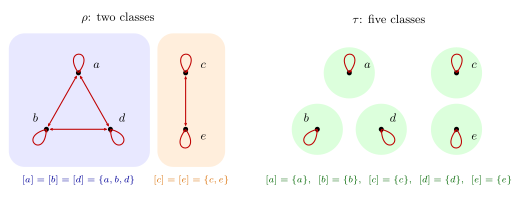
Figure 180: Two equivalence relations on \({a,b,c,d,e}\), with each class shaded. Left: \(\rho\) has 13 pairs, 9 inside \({a,b,d}\) and 4 inside \({c,e}\). A double-headed line stands for an arrow each way. Its classes are the two clusters of the diagram. Right: \(\tau\) keeps only the five loops. It is still reflexive, symmetric and transitive, and each element is in a class by itself. Here \(\tau\) is contained in \(\rho\), and the smaller relation has more, smaller classes.
Common mistakes
- Treating \([a]\) as an element. \([a] \subseteq S\), and \(a \in [a]\). Writing \([a] \in S\) or \([1] = 1\) confuses a set with one of its members (sets-and-set-notation).
- Thinking different names mean different classes. \([0]\) and \([3]\) are the same class mod 3. \(a \neq b\) does not give \([a] \neq [b]\). Only \(a \mathrel{\not\rho} b\) does.
- Giving one example in place of the class. “\([\sqrt2]\) contains \(1 + \sqrt2\)” does not describe \([\sqrt2]\). \(\{y + \sqrt2 : y \in \mathbb{Q}\}\) does.
- Classes that overlap or leave something out. If your list of classes is not a partition of \(S\), something is wrong. Check that each element is in exactly one.
- Taking classes of a relation that is not an equivalence relation. The definition starts “let \(\rho\) be an equivalence relation”. For \(x + y \in \mathbb{Q}\) on \(\mathbb{R}\), the set of things related to \(\sqrt2\) does not even contain \(\sqrt2\).
- An empty part. \(\{\emptyset, \mathbb{Z}\}\) is not a partition of \(\mathbb{Z}\). Parts are non-empty.
See also
- equivalence-relations — the definition, the proof template, and the relations used here
- sets-and-set-notation — partitions as first defined, with more examples
- integers-modulo-n — the classes of congruence mod \(n\) as a number system
- counting-principles — the size of a finite set as the sum of the sizes of the parts of a partition
- reflexive-symmetric-and-transitive-relations — the three properties the proofs here use
- proof-techniques — double containment and proof by contradiction, both used in the equal-or-disjoint proof
- 2026-09-21-equivalence-relations — Lecture 24 · 2026-09-22-partial-order-relations — Lecture 25, which finishes it
- practice-problems — §31, with full worked solutions
Equivalence Relations
A relation that is reflexive, symmetric and transitive at once. Such a relation behaves like “is the same as, in some respect”, and it sorts its set into groups, the equivalence classes of equivalence-classes-and-partitions. The three properties are in reflexive-symmetric-and-transitive-relations. First met in 2026-09-21-equivalence-relations.
The definition
A relation is an equivalence relation if and only if it is: reflexive, symmetric and transitive.
For a relation \(\rho\) on a set \(A\) that is three “for all” statements:
(1) reflexive: \(\forall x \in A,\ x \mathrel{\rho} x\).
(2) symmetric: \(\forall x, y \in A,\ x \mathrel{\rho} y \to y \mathrel{\rho} x\).
(3) transitive: \(\forall x, y, z \in A,\ (x \mathrel{\rho} y \text{ and } y \mathrel{\rho} z) \to x \mathrel{\rho} z\).
All three are needed, and none follows from the other two (reflexive-symmetric-and-transitive-relations).
Relations here are named \(\rho\), \(\tau\), \(\sigma\), \(R\) and \(T\). The symbol \(\sim\) is also used as the name of a relation, as in \((a,b) \sim (c,d)\). It is the same symbol used for not in logic (logical-connectives). Position tells them apart: between two objects it is a relation, and in front of a statement it is a negation.
What the arrow diagram looks like
In the arrow diagram of an equivalence relation every dot has a loop, every arrow has its return, and every two-step path has its short cut. Put together, the diagram falls into separate clusters, with every possible arrow inside a cluster and none between clusters. The clusters are the equivalence classes. The even integers under same parity are a single such cluster (2026-09-21-equivalence-relations). The same shape shows for five real numbers in 2026-09-21-equivalence-relations, and for congruence mod 6 in relations-on-sets.
Figure 181 shows the shape, and one way to break each property.
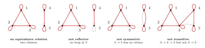
Figure 181: An equivalence relation on \({1,2,3,4,5}\) and three near misses, each differing from it in one place. A double-headed line stands for an arrow each way, and what is missing is dashed. First: two clusters, complete inside, nothing between them. Second: the loop at 5 is removed, so the relation is not reflexive. Third: \(5 \to 4\) is removed, so \(4 \to 5\) has no return and the relation is not symmetric. Fourth: a link between 3 and 4 is added, so the path \(3 \to 4 \to 5\) has no short cut \(3 \to 5\) and the relation is not transitive. A link between two clusters has to be completed until they are one cluster, or removed.
Proving a relation is an equivalence relation
Prove the three properties one at a time, and label each part. Each part is a direct proof of a “for all” statement (proof-techniques):
| Part | Start with | Show |
|---|---|---|
| reflexive | Let \(x \in A\). | \(x \mathrel{\rho} x\) |
| symmetric | Let \(x, y \in A\) and suppose \(x \mathrel{\rho} y\). | \(y \mathrel{\rho} x\) |
| transitive | Let \(x, y, z \in A\) and suppose \(x \mathrel{\rho} y\) and \(y \mathrel{\rho} z\). | \(x \mathrel{\rho} z\) |
In each part, unfold what \(\rho\) means for the elements in hand, work with that, and fold it back into a statement about \(\rho\). Finish with a sentence naming all three: Since \(\rho\) is reflexive, symmetric and transitive, it is an equivalence relation.
Worked: \(x \mathrel{\tau} y \leftrightarrow x - y \in \mathbb{Q}\) on \(\mathbb{R}\)
The proof is written out in full in 2026-09-21-equivalence-relations. Its shape:
- Reflexive. \(x - x = 0 \in \mathbb{Q}\).
- Symmetric. Unfold \(x - y \in \mathbb{Q}\) to \(x - y = \frac{a}{b}\) with \(a, b \in \mathbb{Z}\), \(b \neq 0\). Then \(y - x = \frac{-a}{b} \in \mathbb{Q}\).
- Transitive. Unfold to \(x - y = \frac{a}{b}\) and \(y - z = \frac{c}{d}\). Then \(x - z = (x - y) + (y - z) = \frac{ad + bc}{bd} \in \mathbb{Q}\), with \(bd \neq 0\).
The second fraction gets new letters \(c\), \(d\). The transitive step rests on one identity, \(x - z = (x - y) + (y - z)\), which gets rid of the middle element. Most transitivity proofs need a step like it.
Congruence is the same proof with integers in place of rationals. \(m \mathrel{\rho} n \leftrightarrow d \mid (m - n)\) on \(\mathbb{Z}\) is worked for \(d = 6\) in reflexive-symmetric-and-transitive-relations, and nothing in it depends on the 6.
Worked: a definition with an “or”
\(m \mathrel{\sigma} n \leftrightarrow (8 \mid (m - n)) \text{ or } (8 \mid (m + n))\) on \(\mathbb{Z}\).
The proof is written out in full in 2026-09-21-equivalence-relations. When the definition is an or, every hypothesis of the form \(m \mathrel{\sigma} n\) splits into cases, and each case has to reach the conclusion. A conclusion of the form \(k \mathrel{\sigma} n\) needs only one of its two alternatives.
- Reflexive. No cases: \(8 \mid (m - m)\), the first alternative.
- Symmetric. One hypothesis, two cases. From \(8 \mid (m - n)\) get \(8 \mid (n - m)\). From \(8 \mid (m + n)\) get \(8 \mid (n + m)\).
- Transitive. Two hypotheses, \(2 \times 2 = 4\) cases:
| Case | \(k \mathrel{\sigma} m\) because | \(m \mathrel{\sigma} n\) because | Combine | So 8 divides |
|---|---|---|---|---|
| 1 | \(8 \mid (k - m)\) | \(8 \mid (m - n)\) | add | \(k - n\) |
| 2 | \(8 \mid (k - m)\) | \(8 \mid (m + n)\) | add | \(k + n\) |
| 3 | \(8 \mid (k + m)\) | \(8 \mid (m - n)\) | subtract | \(k + n\) |
| 4 | \(8 \mid (k + m)\) | \(8 \mid (m + n)\) | subtract | \(k - n\) |
In every row the two quantities are added or subtracted, whichever cancels the \(m\).
Disproving
A relation fails to be an equivalence relation as soon as it fails one of the three properties, and a property fails as soon as there is one witness. So a disproof is short: name the property, give specific elements, check them.
\(x \mathrel{\rho} y \leftrightarrow x + y \in \mathbb{Q}\) on \(\mathbb{R}\) is not an equivalence relation: it is not reflexive, because \(\sqrt2 + \sqrt2 = 2\sqrt2 \notin \mathbb{Q}\), so \(\sqrt2 \mathrel{\not\rho} \sqrt2\).
That is the whole answer (2026-09-21-equivalence-relations). Try reflexivity first, since it involves only one element. A relation can fail on any of the three:
| Fails | Relation | Witness | Worked in |
|---|---|---|---|
| reflexive | \(x + y \in \mathbb{Q}\) on \(\mathbb{R}\) | \(\sqrt2 \mathrel{\not\rho} \sqrt2\) | 2026-09-21-equivalence-relations |
| symmetric | \(x\) is a multiple of \(y\), on \(\mathbb{Z}\) | 4 is a multiple of 2, but 2 is not a multiple of 4 | practice-problems, Q1 (\(\beta\)) |
| transitive | \(\lvert x - y \rvert \le 1\) on \(\mathbb{Z}\) | \(0\) and \(1\) are related, \(1\) and \(2\) are related, \(0\) and \(2\) are not | — |
The last one is reflexive and symmetric, and still not an equivalence relation. “Close to” is not transitive, and that is why it never works as a kind of sameness.
“The same …”
Most of the course’s equivalence relations say that two elements have the same something:
| Relation | \(x\) and \(y\) are related when they have the same … |
|---|---|
| \(m \equiv n \pmod 3\) on \(\mathbb{Z}\) | remainder on division by 3 |
| same parity on \(\mathbb{Z}\) | parity |
| in the same part of a partition | part |
| \((a,b) \sim (c,d) \leftrightarrow ad = bc\) | value as a fraction |
| \(R_n\) on strings | first \(n\) characters (practice-problems, Q3) |
| \(x = y\) on any set | identity |
A relation of the form “\(x\) and \(y\) have the same value of \(f\)”, that is \(f(x) = f(y)\) for some function \(f\) on the set, is always an equivalence relation, because the three properties are inherited from \(=\): \(f(x) = f(x)\); if \(f(x) = f(y)\) then \(f(y) = f(x)\); and if \(f(x) = f(y)\) and \(f(y) = f(z)\) then \(f(x) = f(z)\). Recognising this shape tells you the answer is yes before you start. The proof still has to be written out for the relation as given.
Not every example is given in that form. \(x - y \in \mathbb{Q}\) and the relation \(\sigma\) above have to be proved from their definitions.
The same fraction
An equivalence relation that is neither congruence nor equality:
\((a,b) \sim (c,d)\ \) if and only if \(\ ad = bc\)
The set is \(\mathbb{Z}^{+} \times \mathbb{Z}^{+}\), pairs of positive integers, with \((a,b)\) standing for the fraction \(\frac{a}{b}\). Two pairs are related when cross-multiplying gives equal products. The condition \(ad = bc\) says \(\frac{a}{b} = \frac{c}{d}\) without dividing, so it stays inside the integers. For example \(\frac12 = \frac24 = \frac36\), so \((1,2)\), \((2,4)\) and \((3,6)\) are all related.
- Reflexive. Let \((a,b) \in \mathbb{Z}^{+} \times \mathbb{Z}^{+}\). Then \(ab = ba\), so \((a,b) \sim (a,b)\).
- Symmetric. Suppose \((a,b) \sim (c,d)\), so \(ad = bc\). Then \(cb = da\), so \((c,d) \sim (a,b)\).
- Transitive. Suppose \((a,b) \sim (c,d)\) and \((c,d) \sim (e,f)\), so \(ad = bc\) and \(cf = de\). Then \[(af)d = (ad)f = (bc)f = b(cf) = b(de) = (be)d,\] and since \(d \neq 0\) we may cancel it: \(af = be\). So \((a,b) \sim (e,f)\).
Each equivalence class is one positive rational number, with all the ways of writing it: \([(1,2)] = \{(1,2), (2,4), (3,6), \dots\}\). So the positive rationals \(\mathbb{Q}^{+}\) can be built as the classes of this relation. The figure below draws the classes as rays.
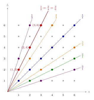
Figure 182: The pairs \((a,b)\) with \(a\) and \(b\) from 1 to 6, plotted as points. Two pairs satisfy \(ad = bc\) exactly when they lie on the same line through the origin, so the equivalence classes are the rays out of the origin, and each ray is one positive rational. The red ray holds \((1,2)\), \((2,4)\) and \((3,6)\), the three fractions of \(\tfrac12 = \tfrac24 = \tfrac36\). Six more rays are coloured and labelled with their fraction. Every grey point is on a ray of its own within this window.
The examples side by side
| Relation | on | Equivalence relation? | Classes |
|---|---|---|---|
| \(m \equiv n \pmod 3\) | \(\mathbb{Z}\) | yes | \([0]\), \([1]\), \([2]\) |
| same parity | \(\mathbb{Z}\) | yes | \(\mathbb{Z}^{even}\), \(\mathbb{Z}^{odd}\) |
| \(x - y \in \mathbb{Q}\) | \(\mathbb{R}\) | yes | \([a] = \{y + a : y \in \mathbb{Q}\}\), infinitely many |
| \(8 \mid (m - n)\) or \(8 \mid (m + n)\) | \(\mathbb{Z}\) | yes | five: \([0]\), \([1]\), \([2]\), \([3]\), \([4]\) |
| in the same part of \(\{\{1,2,3\},\{4,5\},\{6\}\}\) | \(\{1,\dots,6\}\) | yes | the three parts |
| \(ad = bc\) | \(\mathbb{Z}^{+} \times \mathbb{Z}^{+}\) | yes | one for each positive rational |
| \(x = y\) | any set | yes | one for each element, \([a] = \{a\}\) |
| \(3 \mid (x^2 - y^2)\) | \(\mathbb{Z}\) | yes | multiples of 3, non-multiples of 3 |
| \(x + y \in \mathbb{Q}\) | \(\mathbb{R}\) | no, not reflexive | — |
| \(x\) is a multiple of \(y\) | \(\mathbb{Z}\) | no, not symmetric | — |
The classes for the first five rows and the ninth are worked in equivalence-classes-and-partitions. The eighth and tenth are \(\gamma\) and \(\beta\) of practice-problems, Q1.
Common mistakes
- Proving two properties and stopping, or checking a property on a few examples. Each property is a “for all”, and needs a general argument about arbitrary elements.
- Assuming the conclusion in the symmetric part. The hypothesis is only \(x \mathrel{\rho} y\). \(y \mathrel{\rho} x\) is what has to come out.
- Reusing a letter when unfolding twice. \(x - y = \frac{a}{b}\) and \(y - z = \frac{a}{b}\) would say the two differences are equal. Use \(\frac{c}{d}\).
- Skipping reflexivity because “symmetric and transitive give it”. They do not (reflexive-symmetric-and-transitive-relations).
- Disproving without a witness. “It isn’t always true that \(x + x\) is rational” is not a disproof. \(x = \sqrt2\) is.
- Forgetting the set. The same rule on a different set is a different relation. \(x + y \in \mathbb{Q}\) fails on \(\mathbb{R}\), but on \(\mathbb{Q}\) every pair is related and it is an equivalence relation with a single class.
See also
- equivalence-classes-and-partitions — the classes of an equivalence relation, and why they partition the set
- reflexive-symmetric-and-transitive-relations — the three properties, one at a time
- relations-on-sets — relations as sets of pairs, and arrow diagrams
- partial-order-relations — the other important kind of relation, with antisymmetric in place of symmetric
- modular-arithmetic · integers-modulo-n — congruence, and its classes as the elements of \(\mathbb{Z}_n\)
- rational-and-irrational-numbers — the definition of rational that the \(x - y \in \mathbb{Q}\) proof unfolds
- 2026-09-21-equivalence-relations — Lecture 24
- practice-problems — §31, with full worked solutions
Euler Circuits and Trails
An Euler circuit goes along every edge of a graph exactly once and comes back to where it started. An Euler trail does the same but finishes somewhere else. Whether a graph has one is decided by two things only: whether it is connected once its isolated vertices are set aside, and how many of its vertices have odd degree. None gives an Euler circuit, exactly two gives an Euler trail from one of them to the other, and any other number gives neither. This note has the definitions, the theorem with a full proof, how to actually find a circuit or trail, a flowchart for deciding, and how this course’s definition differs from the textbook’s. It builds on walks, trails, circuits and connectedness in walks-trails-and-circuits, and on degree in graphs. First met in 2026-10-26-walks-trails-and-circuits.
Euler circuits
An Euler circuit is a circuit that contains every edge of the graph.
A circuit never uses an edge twice (walks-trails-and-circuits), so an Euler circuit uses every edge exactly once and ends where it started. It may pass through a vertex many times. A graph that has an Euler circuit is called Eulerian.
A graph with no edges has an Euler circuit: the trivial circuit at any vertex contains every edge, since there are none.
Euler trails
An Euler trail from vertex \(u\) to vertex \(v\) is a trail that starts at \(u\) and ends at \(v\) and contains every edge of the graph.
The difference from an Euler circuit is only where it finishes. Both use every edge exactly once. An Euler circuit ends at the vertex it started from. An Euler trail from \(u\) to \(v\) ends at \(v\), and the case that matters is \(u \ne v\), an open route. (An Euler circuit is a trail from a vertex to itself, but the theorem below is about \(u \ne v\).)
For a connected graph the two cannot both happen with \(u \ne v\): the theorem says an Euler circuit needs every degree even, and an Euler trail from \(u\) to \(v \ne u\) needs \(u\) and \(v\) odd.
The theorem
Theorem. Let \(G\) be a connected graph. Then \(G\) has an Euler circuit if and only if every vertex of \(G\) has even degree.
Let \(u, v \in V(G)\) be distinct vertices of \(G\). Then \(G\) has an Euler trail from \(u\) to \(v\) if and only if \(u\) and \(v\) have odd degree and all other vertices of \(G\) have even degree.
Every graph has an even number of vertices of odd degree (graphs), so for a connected graph there are three cases: no odd vertices gives an Euler circuit, exactly two gives an Euler trail between them, and four or more gives neither.
Counting edge ends along a trail
Both directions of the proof rest on one count. Take a trail \(T = v_0\, e_1\, v_1 \cdots e_n\, v_n\) and a vertex \(w\). The edge \(e_i\) has its two ends at \(v_{i-1}\) and \(v_i\) (both at the same vertex if it is a loop). So the number of edge ends at \(w\) that \(T\) uses is
\[\underbrace{\#\{\, i : v_{i-1} = w \,\}}_{\text{times } T \text{ leaves } w} \;+\; \underbrace{\#\{\, i : v_i = w \,\}}_{\text{times } T \text{ arrives at } w}.\]
These ends are all different, because the edges of a trail are all different. Reading along the sequence, each arrival at \(w\) is followed by a departure, except an arrival at the very end, and each departure is preceded by an arrival, except a departure at the very start. So:
- If \(w\) is not the first or last vertex, \(T\) arrives at \(w\) exactly as often as it leaves: every pass through \(w\) uses two ends, one in and one out, and the number used is even.
- If \(T\) is a circuit (\(v_0 = v_n\)), the departure at the start and the arrival at the end pair up at \(v_0\), and every vertex has an even number of ends used.
- If \(v_0 \ne v_n\), \(T\) leaves \(v_0\) once more than it arrives, and arrives at \(v_n\) once more than it leaves. At those two vertices the number of ends used is odd.
A loop at \(w\) is an arrival at \(w\) and a departure from \(w\) at once, and uses two ends at \(w\), so it never changes these parities.
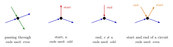
Figure 183: Edge ends used by a trail at one vertex. Arrows show the direction of travel. Left: a vertex in the middle of the trail. Each time the trail passes through, it arrives along one edge and leaves along another, so the ends pair up, blue with blue and green with green, and an even number is used. Second: the start of a trail that ends elsewhere has one departure with no arrival to pair with, in red, so an odd number is used. Third: the end of such a trail has one arrival left over. Right: at the start of a circuit, the first departure pairs with the final arrival, so every end pairs up again.
Proof: every edge used forces the degrees
Proof that an Euler circuit or trail forces the degrees. Suppose \(T\) is an Euler circuit of \(G\). It uses every edge exactly once, so it uses every edge end in \(G\) exactly once, and the number of ends it uses at a vertex \(w\) is all of them, \(\deg(w)\). By the count above that number is even. So every vertex has even degree.
Suppose instead \(T\) is an Euler trail from \(u\) to \(v\) with \(u \ne v\). Again the ends used at \(w\) number \(\deg(w)\). By the count, that is odd for \(w = u\) and \(w = v\), and even for every other vertex. \(\square\)
This direction does not use connectedness.
Proof: even degrees give an Euler circuit
The construction rests on one fact about walking until stuck.
Lemma (stuck only at the start). Let \(H\) be a graph in which every vertex has even degree, and \(w\) a vertex with \(\deg(w) \ge 1\). Start at \(w\) and build a trail one edge at a time: from the current vertex, go along any edge at it that has not been used yet, and stop when there is none. Then this stops, and it stops at \(w\), so it produces a non-trivial circuit through \(w\).
Proof. Each step uses a new edge and there are finitely many, so it stops. Suppose it is at a vertex \(x \ne w\), having arrived there. The trail so far starts at \(w\) and ends at \(x \ne w\), so by the count it has used an odd number of the ends at \(x\). Since \(\deg(x)\) is even, some end at \(x\) is unused, and the edge it belongs to is unused, because an edge is used all at once. So the trail can go on, and it does not stop at \(x\). It therefore stops at \(w\). It started along an edge, since \(\deg(w) \ge 1\), so the circuit has at least one edge. \(\square\)
Removing a circuit keeps every degree even. If \(C\) is a circuit and its edges are deleted (keeping all the vertices), each vertex loses the ends of it that \(C\) used, an even number by the count. Even minus even is even.
Proof of the theorem, circuits. Let \(G\) be connected with every vertex of even degree. Every vertex is a trivial circuit, so \(G\) has circuits. A circuit uses each edge at most once, so it has at most \(|E(G)|\) edges, and there is a circuit \(C = v_0\, e_1\, v_1 \cdots e_n\, v_n\) with as many edges as possible. Suppose, for a contradiction, that some edge of \(G\) is not in \(C\).
Let \(H\) be \(G\) with the edges of \(C\) deleted. \(H\) has every vertex of even degree and at least one edge.
Some vertex of \(C\) has an edge in \(H\). Take an edge of \(H\) and an endpoint \(x\) of it. If \(x\) is on \(C\), done. If not, \(G\) is connected, so there is a walk in \(G\) from \(x\) to \(v_0\). The walk starts off \(C\) and ends on \(C\), so there is a first vertex \(y\) on it that lies on \(C\), and the vertex \(z\) just before \(y\) is not on \(C\). The edge \(f\) of the walk joining \(z\) and \(y\) is not an edge of \(C\), since every edge of \(C\) has both endpoints on \(C\). So \(f\) is in \(H\), and its endpoint \(y\) is on \(C\). Call this vertex \(w\).
Splice. \(w\) has degree at least 1 in \(H\), so the lemma, applied in \(H\), gives a non-trivial circuit \(C' = w\, f_1\, u_1 \cdots f_m\, w\) using only edges of \(H\). \(w\) is on \(C\), say \(w = v_k\). Replace that one occurrence of \(v_k\) in \(C\) by the whole of \(C'\):
\[v_0\, e_1\, v_1 \cdots e_k\, \underbrace{v_k\, f_1\, u_1 \cdots f_m\, v_k}_{C'}\, e_{k+1} \cdots e_n\, v_n.\]
This is a walk, since \(C'\) leaves from \(v_k\) and returns to \(v_k\). Its edges are those of \(C\) and those of \(C'\), which are all different, since the edges of \(C'\) are in \(H\) and \(H\) has none of the edges of \(C\). So it is a trail, and it starts and ends at \(v_0 = v_n\), so it is a circuit. It has \(n + m > n\) edges, contradicting the choice of \(C\).
So \(C\) contains every edge of \(G\), and it is an Euler circuit. \(\square\)
If \(G\) has no edges, \(C\) is a trivial circuit and nothing is missing. Connectedness is used in exactly one place: to get from an unused edge back to the circuit.
Proof: two odd vertices give an Euler trail
Proof of the theorem, trails. Let \(G\) be connected, with \(u \ne v\) of odd degree and every other vertex of even degree. Make a new graph \(G'\) by adding one new edge \(f\) with endpoints \(u\) and \(v\). If \(u\) and \(v\) are already adjacent, \(f\) is a parallel edge, and that is fine. In \(G'\), \(u\) and \(v\) each gain one end, so every vertex of \(G'\) has even degree, and \(G'\) is still connected. By the circuit case, \(G'\) has an Euler circuit \(C\).
\(C\) uses \(f\) once, either as \(\cdots u\, f\, v \cdots\) or as \(\cdots v\, f\, u \cdots\). Read backwards if necessary (walks-trails-and-circuits) so that it is \(\cdots v\, f\, u \cdots\). Then start the circuit at that \(u\), so that \(f\) is the last edge:
\[C = u \cdots v\, f\, u.\]
Delete the final \(f\, u\). What is left is a trail, since its edges are some of the distinct edges of \(C\). It starts at \(u\), ends at \(v\), uses every edge of \(G'\) except \(f\) exactly once, and so uses every edge of \(G\) exactly once. It is an Euler trail from \(u\) to \(v\). \(\square\)
Together with the first direction, that proves the theorem.
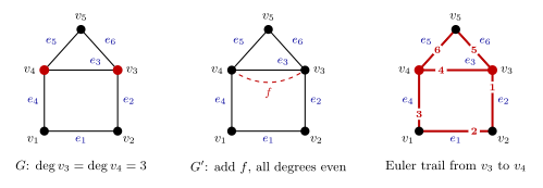
Figure 184: The trail case from the circuit case. Left: the house graph, connected, with \(v_3\) and \(v_4\) of odd degree, in red, and the others even. Middle: adding a new edge \(f\) joining \(v_3\) and \(v_4\), dashed, makes every degree even, so there is an Euler circuit, for example \(v_3, e_2, v_2, e_1, v_1, e_4, v_4, e_3, v_3, e_6, v_5, e_5, v_4, f, v_3\), which ends with \(f\). Here \(f\) is a second edge between two vertices that were already adjacent. Right: drop the final \(f\). What is left, \(v_3, e_2, v_2, e_1, v_1, e_4, v_4, e_3, v_3, e_6, v_5, e_5, v_4\), is an Euler trail from \(v_3\) to \(v_4\), in red with its edges numbered in order.
This course’s definition and the textbook’s
This course uses the standard definitions above: an Euler circuit contains every edge. The textbook defines an Euler circuit as a circuit that contains every vertex and every edge of the graph, and an Euler trail likewise.
They differ only when there are vertices that no edge touches. A triangle together with one isolated vertex has an Euler circuit by this course’s definition (go once round the triangle), and none by the textbook’s, because no circuit can reach the isolated vertex.
Figure 185: A triangle and an isolated vertex \(z\). Going once round the triangle, in red, uses every edge, so by this course’s definition it is an Euler circuit. By the textbook’s definition it is not, since it misses \(z\), and no circuit can visit \(z\). The graph is disconnected, so the theorem does not apply to it as it stands. Deleting \(z\) leaves a connected graph with all degrees even.
For a connected graph the two definitions agree. A circuit or trail that contains every vertex and every edge certainly contains every edge. Conversely, let \(G\) be connected and let \(T\) contain every edge.
- If \(G\) has at least one edge, then every vertex is the endpoint of some edge. With a single vertex, every edge is a loop at it. With two or more vertices, take any vertex \(x\) and another vertex \(y\): there is a walk from \(x\) to \(y\), and its first edge has \(x\) as an endpoint. \(T\) uses that edge, so \(T\) passes through \(x\).
- If \(G\) has no edges, being connected means it has one vertex. The only walk in \(G\) is that single vertex, so \(T\) is the trivial circuit there, and it contains the vertex.
So \(T\) contains every vertex too. The theorem assumes \(G\) is connected, so it says the same thing under either definition. The definitions only part ways for disconnected graphs whose edges all lie in one piece, with isolated vertices as the rest, such as the triangle and isolated vertex, and that case is what the first two steps of the flowchart deal with.
How to find one
The theorem says whether an Euler circuit or trail exists. To write one down, I use the splicing method that the proof is built on (it is usually called Hierholzer’s algorithm):
- Check first. Delete isolated vertices, check the rest is connected, and count the vertices of odd degree. None: look for a circuit, starting anywhere. Two, \(u\) and \(v\): look for a trail, starting at \(u\).
- Walk until stuck. From the start, keep going along edges not used yet, choosing freely, until there are none at the current vertex. For a circuit this always stops back at the start (the lemma). For a trail from \(u\) it always stops at \(v\): by the count, at any other vertex the trail has used an odd number of ends of an even-degree vertex, or, at \(u\), an even number of ends of an odd-degree vertex, and either way an end is left.
- If edges are left, splice. The unused edges give every vertex even degree, since what was walked used an even number of ends at each vertex except \(u\) and \(v\), and an odd number at those two. Pick a vertex already on the route that still has an unused edge. Walk from it along unused edges until stuck. That is back at the same vertex. Insert this circuit into the route at that vertex.
- Repeat step 3 until every edge is used.
When walking, it helps to tick off each edge on the drawing as it is used, and to write the route as a list of vertices (with edge names where there are multiple edges).
Another method avoids splicing by choosing carefully as you go (Fleury’s algorithm): walk from the start, and at each step don’t burn your bridges, that is, never use an edge whose removal would cut the unused edges into two separate pieces, unless it is the only edge left at the vertex. It gives the circuit or trail in one pass, but checking every step for a bridge is slow by hand, so I splice.
Worked: an Euler circuit by splicing
Find an Euler circuit of the graph below: six vertices, each joined to every other vertex except one, the vertex “opposite” it. The non-adjacent pairs are \(v_1, v_6\); \(v_2, v_4\); \(v_3, v_5\).
There are 12 edges, \(v_1v_2, v_1v_3, v_1v_4, v_1v_5, v_2v_3, v_2v_5, v_2v_6, v_3v_4, v_3v_6, v_4v_5, v_4v_6, v_5v_6\). The graph is connected and every vertex has degree 4, so there is an Euler circuit. The graph is simple, so a route can be written as a list of vertices.
Walk until stuck. From \(v_1\):
\[v_1\, v_2\, v_3\, v_1\, v_4\, v_5\, v_1.\]
At \(v_1\) all four edges are now used, so this is stuck, back at the start, with 6 edges. Left over: \(v_2v_5, v_2v_6, v_3v_4, v_3v_6, v_4v_6, v_5v_6\).
First splice. \(v_2\) is on the route and still has the unused edges \(v_2v_5\) and \(v_2v_6\). Walk from \(v_2\) along unused edges: \(v_2\, v_5\, v_6\, v_2\), stuck at \(v_2\). Insert it where the route passes \(v_2\):
\[v_1\, \underbrace{v_2\, v_5\, v_6\, v_2}_{\text{inserted}}\, v_3\, v_1\, v_4\, v_5\, v_1.\]
Left over: \(v_3v_4, v_3v_6, v_4v_6\).
Second splice. \(v_3\) is on the route and still has unused edges. Walk from it: \(v_3\, v_4\, v_6\, v_3\). Insert it where the route passes \(v_3\):
\[v_1\, v_2\, v_5\, v_6\, v_2\, \underbrace{v_3\, v_4\, v_6\, v_3}_{\text{inserted}}\, v_1\, v_4\, v_5\, v_1.\]
That uses all 12 edges, each once, and returns to \(v_1\): an Euler circuit.
Figure 186: Finding an Euler circuit by splicing. Red: the first circuit, \(v_1,v_2,v_3,v_1,v_4,v_5,v_1\), walked from \(v_1\) until stuck. Blue: the circuit \(v_2,v_5,v_6,v_2\) through \(v_2\), built from unused edges and spliced in at \(v_2\). Green: the circuit \(v_3,v_4,v_6,v_3\) through \(v_3\), spliced in at \(v_3\). The small numbers give the order of the edges in the final circuit, \(v_1,v_2,v_5,v_6,v_2,v_3,v_4,v_6,v_3,v_1,v_4,v_5,v_1\).
Deciding: the flowchart
For any graph, connected or not:
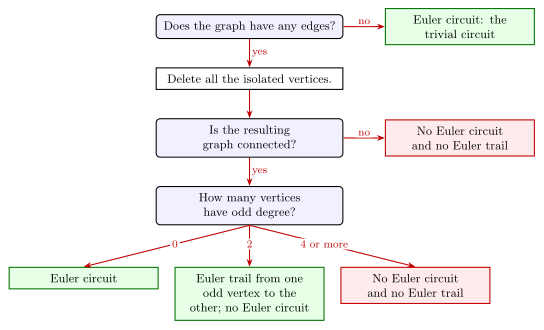
Figure 187: Deciding whether a graph has an Euler circuit or an Euler trail. A graph with no edges has one, the trivial circuit. Otherwise isolated vertices are deleted, since no edge touches them, and what is left must be connected, or some two edges cannot be on one route. Then the number of vertices of odd degree decides, and it is always even: none gives an Euler circuit, exactly two gives an Euler trail from one to the other, and four or more gives neither.
Why each step is right:
- No edges. The trivial circuit at any vertex contains every edge, so there is an Euler circuit. This uses this course’s definition: by the textbook’s, a graph with two or more vertices and no edges would have none.
- Deleting isolated vertices changes no edge, so it does not change which routes use every edge. A route that uses every edge never needs to visit an isolated vertex.
- Not connected, after deleting isolated vertices. Then there are vertices \(x\) and \(y\) with no walk between them, and each has an edge, since nothing isolated is left. A circuit or trail containing both edges would contain a walk from \(x\) to \(y\). So there is neither.
- Connected. Now the theorem applies. The number of odd-degree vertices is even (graphs), so 0, 2, or 4 or more covers everything.
The bridges of Königsberg
The problem that started graph theory: the city of Königsberg had four land masses joined by seven bridges, and the question was whether there is a walk around the city crossing every bridge exactly once, ideally returning to the start. As a graph, the land masses are the vertices and the bridges the edges. The island has degree 5 and each of the other three land masses has degree 3 (2026-10-26-walks-trails-and-circuits has the graph).
All four vertices have odd degree. The graph is connected, so by the theorem there is no Euler circuit, since that needs every degree even, and no Euler trail either, since that needs exactly two odd vertices. No walk crosses every bridge exactly once, whether or not it returns. The problem is set up in 2026-07-27-welcome-and-intro-problems.
Common mistakes
- Forgetting connectedness. Even degrees are not enough. Two separate circuits, such as two triangles, have every degree even and no Euler circuit. Check that the graph is connected, after deleting isolated vertices, before using the degrees.
- Letting isolated vertices decide. An isolated vertex makes the graph disconnected but does not stop an Euler circuit, by this course’s definition. Delete them first. (By the textbook’s definition they do stop one, which is why the definitions are compared above.)
- Counting a loop as 1. A loop adds 2 to the degree (graphs), so loops never change whether a degree is odd or even.
- Exactly two odd vertices gives a trail, not a circuit. The trail must start at one odd vertex and end at the other. Starting at an even vertex will not work.
- Zero odd vertices gives a circuit, and the trail part of the theorem does not apply. An Euler circuit is also a trail from a vertex to itself, but the trail statement in the theorem is about \(u \ne v\). With every degree even there is no Euler trail from \(u\) to a different \(v\), since that would need \(u\) and \(v\) odd.
- Getting stuck and concluding there is none. Walking until stuck can leave edges unused even when an Euler circuit exists. That is not a failure: splice in the rest (how to find one). Only the degrees and connectedness decide existence.
See also
- walks-trails-and-circuits — walks, trails, circuits and connected graphs
- [graphs] — degree, loops and the Handshake Theorem
- 2026-10-26-walks-trails-and-circuits — Lecture 34, with worked questions on the theorem and an Euler trail on ten vertices
- 2026-07-27-welcome-and-intro-problems — the bridges of Königsberg
- [trees] — connected graphs with no non-trivial circuits
- practice-problems — §44, with full worked solutions
Fields
A field is a set with two operations, \(+\) and \(\cdot\), in which you can add, subtract, multiply, and divide by anything except 0, with all the usual rules holding. Formally it is two abelian [groups] on one set, \((F, +)\) on all of it and \((F - \{0\}, \cdot)\) on everything but 0, tied together by the distributive laws. \(\mathbb{Q}\) and \(\mathbb{R}\) are fields, \(\mathbb{Z}\) is not, and \(\mathbb{Z}_n\) (integers-modulo-n) is a field exactly when \(n\) is prime. In a field every linear equation \(ax + b = c\) with \(a \neq 0\) has exactly one solution. First met in 2026-10-08-definitions-and-examples-of-fields.
The definition
Definition. A field \((F, +, \cdot)\) is a set \(F\) with two binary operations \(+\) and \(\cdot\) such that
(1) \((F, +)\) is an abelian group;
(2) \((F - \{0\}, \cdot)\) is an abelian group, where \(0\) is the identity of \((F, +)\); and
(3) for all \(f, g, h \in F\), \(\ f \cdot (g + h) = (f \cdot g) + (f \cdot h)\) and \((f + g) \cdot h = (f \cdot h) + (g \cdot h)\).
Written out, conditions (1) and (2) are five checks each, side by side:
| Addition, on \(F\) | Multiplication, on \(F - \{0\}\) | |
|---|---|---|
| closure | \(f + g \in F\) | \(f, g \neq 0 \Rightarrow f \cdot g \neq 0\) |
| associativity | \((f + g) + h = f + (g + h)\) | \((f \cdot g) \cdot h = f \cdot (g \cdot h)\) |
| identity | \(0\), with \(0 + f = f + 0 = f\) | \(1\), with \(1 \cdot f = f \cdot 1 = f\) |
| inverses | every \(f\) has \(-f\), with \(f + (-f) = 0\) | every \(f \neq 0\) has \(f^{-1}\), with \(f \cdot f^{-1} = 1\) |
| commutativity | \(f + g = g + f\) | \(f \cdot g = g \cdot f\) |
Condition (3) is the two distributive laws, which hold for all \(f, g, h \in F\), zero included.
Points that are easy to read past:
- The two identities are named 0 and 1 by their jobs, not because they are the integers 0 and 1. In \(\mathbb{Z}_n\) they are \([0]\) and \([1]\). The “0” removed in condition (2) is whatever the additive identity is.
- Closure in (2) is a real condition. It says that a product of two non-zero elements is never 0. It is the condition \(\mathbb{Z}_4\) and \(\mathbb{Z}_{15}\) fail.
- \(-f\) and \(f^{-1}\) are different inverses. Each element has an additive inverse, and each non-zero element has a multiplicative one as well. In \(\mathbb{Z}_5\), \(-[2] = [3]\) and \([2]^{-1} = [3]\) happen to agree, but \(-[4] = [1]\) while \([4]^{-1} = [4]\).
- The distributive laws are the only link between the operations. Without (3), a field would be two unrelated groups that happen to share a set.
Why 0 is left out of (2). In any field, \(0 \cdot f = 0\) for every \(f\). By the distributive law, \[0 \cdot f = (0 + 0) \cdot f = (0 \cdot f) + (0 \cdot f),\] and adding \(-(0 \cdot f)\) to both sides leaves \(0 = 0 \cdot f\). So \(0 \cdot y = 1\) has no solution, and 0 can never have a multiplicative inverse. Asking for a group on all of \(F\) under \(\cdot\) would rule out every field, just as 0 stops \((\mathbb{R}, \cdot)\) being a group (groups).
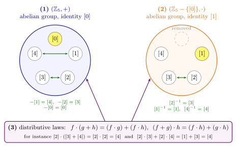
Figure 188: A field is two abelian groups on one set, shown for \(\mathbb{Z}_5\). Left: all five classes under addition, identity \([0]\). A line joins each class to its additive inverse; \([0]\) is its own. Right: the same classes under multiplication, with \([0]\) taken out and identity \([1]\). \([2]\) and \([3]\) are inverses, and \([1]\) and \([4]\) are their own. The same class can have different inverses in the two groups: \(-[4] = [1]\) but \([4]^{-1} = [4]\). Below: the distributive laws, the one condition that mentions both operations, checked on one instance.
Examples and non-examples
| Field? | Why | |
|---|---|---|
| \((\mathbb{Q}, +, \cdot)\) | yes | every non-zero \(\frac{a}{b}\) has inverse \(\frac{b}{a}\) |
| \((\mathbb{R}, +, \cdot)\) | yes | every non-zero \(x\) has inverse \(\frac1x\) |
| \((\mathbb{Z}, +, \cdot)\) | no | 2 has no multiplicative inverse in \(\mathbb{Z}\) |
| \((\mathbb{Z}_7, +, \cdot)\) | yes | 7 is prime |
| \((\mathbb{Z}_4, +, \cdot)\) | no | \([2] \cdot [2] = [0]\): closure fails in (2) |
| \((\mathbb{Z}_{15}, +, \cdot)\) | no | \([3] \cdot [5] = [0]\): closure fails in (2) |
| \((\mathbb{Z}_{12}, +, \cdot)\) | no | \([2]\) has no inverse, since \(2k\) is even and never \(\equiv 1 \pmod{12}\) |
\(\mathbb{Z}\), \(\mathbb{Z}_4\), \(\mathbb{Z}_7\) and \(\mathbb{Z}_{15}\) are worked in 2026-10-08-definitions-and-examples-of-fields and 2026-10-08-definitions-and-examples-of-fields. \(\mathbb{Z}_{12}\) is Q2 of practice-problems, and Q3 of the same set checks every condition for an unfamiliar field on \(\mathbb{Q} \times \mathbb{Q}\).
Every one of the non-examples passes (1) and (3) and fails (2). That is the usual pattern: addition is rarely the problem, and the work in deciding whether something is a field is in the multiplicative group.
To show something is not a field, one failure with specific elements is enough, as for groups: “2 has no inverse in \(\mathbb{Z}\)”, or “\([3] \cdot [5] = [0]\) in \(\mathbb{Z}_{15}\)”.
\(\mathbb{Z}_n\) is a field exactly when \(n\) is prime
\((\mathbb{Z}_n, +)\) is a group for every \(n \in \mathbb{Z}^{+}\).
\((\mathbb{Z}_p, +, \cdot)\) is a field when \(p\) is prime.
For any \(n\), condition (1) holds (integers-modulo-n), and condition (3), associativity, commutativity and the identity \([1]\) for multiplication are all inherited from the integers, for example \([a]([b] + [c]) = [a(b + c)] = [ab + ac] = [a][b] + [a][c]\). So whether \(\mathbb{Z}_n\) is a field comes down to two things about \(\mathbb{Z}_n - \{[0]\}\): is it closed under multiplication, and does every class in it have an inverse?
When \(n\) is composite, closure fails. Write \(n = rs\) with \(1 < r, s < n\). Then \([r]\) and \([s]\) are non-zero, but \[[r] \cdot [s] = [rs] = [n] = [0].\] \(\mathbb{Z}_4\) (\(2 \cdot 2\)), \(\mathbb{Z}_6\) (\(2 \cdot 3\)), \(\mathbb{Z}_{12}\) (\(3 \cdot 4\)) and \(\mathbb{Z}_{15}\) (\(3 \cdot 5\)) all fail this way. A non-zero class that multiplies something non-zero into \([0]\) also has no inverse: if \([a][b] = [0]\) with \([b] \neq [0]\), multiplying both sides by an inverse of \([a]\) would give \([b] = [0]\). That is why \([2]\), with \([2][6] = [0]\), has no inverse in \(\mathbb{Z}_{12}\).
When \(n = p\) is prime, both hold.
- Closure. If \([a] \cdot [b] = [0]\) then \(p \mid ab\). The prime \(p\) appears in the prime factorisation of \(ab\), which is the factorisation of \(a\) together with that of \(b\) (divisibility-and-factorisation), so \(p \mid a\) or \(p \mid b\). That is, \([a] = [0]\) or \([b] = [0]\). A product of non-zero classes is non-zero.
- Inverses. Fix \([a] \neq [0]\) and look at its row of the table, \([a][1], [a][2], \dots, [a][p-1]\). By closure none of these is \([0]\). No two are equal: if \([a][b] = [a][c]\) then \(p \mid a(b - c)\), and since \(p \nmid a\), the same argument gives \(p \mid (b - c)\), so \([b] = [c]\). That is \(p - 1\) different non-zero classes, which is all of them, so one of them is \([1]\). Whichever \([b]\) gives it is \([a]^{-1}\).
So \(\mathbb{Z}_n\) is a field for \(n = 2, 3, 5, 7, 11, 13, \dots\) and for no other \(n \geq 2\). (\(\mathbb{Z}_1\) has one class, \(\mathbb{Z}_1 - \{[0]\}\) is empty, and the empty set has no identity, so it is not a field either.)
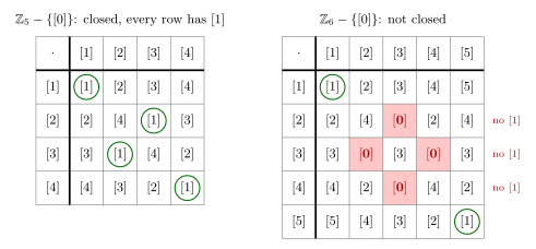
Figure 189: Multiplication on the non-zero classes of \(\mathbb{Z}_5\) and of \(\mathbb{Z}_6\). Left, \(p = 5\) prime: no product is \([0]\), so the set is closed, and \([1]\) (ringed) appears once in every row and every column, so every class has an inverse. Right, \(n = 6 = 2 \cdot 3\): the red cells are products of two non-zero classes that come out as \([0]\), so closure fails. The rows of \([2]\), \([3]\) and \([4]\), the classes sharing a factor with 6, contain no \([1]\), so those classes have no inverse. Only \([1]\) and \([5]\) do.
Calculating in a field
The two inverses give the other two operations:
- Subtraction is adding the additive inverse: \(f - g = f + (-g)\).
- Division is multiplying by the multiplicative inverse: \(f \div g = f \cdot g^{-1}\), for \(g \neq 0\).
In \(\mathbb{Q}\) and \(\mathbb{R}\) these are the familiar operations. In \(\mathbb{Z}_p\):
- \(-[a] = [-a] = [p - a]\). In \(\mathbb{Z}_{11}\), \(-[3] = [8]\), because \([3] + [8] = [11] = [0]\).
- \([a]^{-1}\) is the class \([b]\) with \(ab \equiv 1 \pmod p\). It is never a fraction: in \(\mathbb{Z}_{11}\), \([2]^{-1} = [6]\), because \(2 \cdot 6 = 12 \equiv 1\). Ways to find it are in integers-modulo-n.
So “\(5 \div 2\)” in \(\mathbb{Z}_{11}\) is \([5] \cdot [6] = [30] = [8]\), and indeed \([2] \cdot [8] = [16] = [5]\).
Solving linear equations
To solve \(ax + b = c\) in a field, with \(a \neq 0\):
- Add \(-b\) to both sides, which exists by (1): \(ax = c + (-b)\).
- Multiply both sides by \(a^{-1}\), which exists by (2) because \(a \neq 0\): \(x = a^{-1} \cdot (c + (-b))\).
- Check by substituting back.
Each step is reversible, since \(b\) and \(a\) can be put back by adding \(b\) and multiplying by \(a\). So the equation has exactly one solution, \(x = a^{-1}(c - b)\). It is the two-group version of solving \(a * x = b\) in a group (groups).
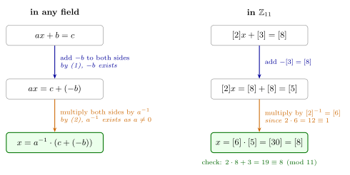
Figure 190: Solving \(ax + b = c\) in a field, on the left in general and on the right for \(2x + 3 = 8\) in \(\mathbb{Z}_{11}\). Each arrow applies one inverse to both sides. The first uses the additive group, condition (1): every element, here \([3]\), has a negative, \([-3] = [8]\). The second uses the multiplicative group, condition (2): every non-zero element, here \([2]\), has an inverse, \([6]\). Neither step can fail in a field, so the equation always has exactly one solution.
Worked: an equation in \(\mathbb{Z}_{13}\)
Solve \(5x + 7 = 3\) in the field \((\mathbb{Z}_{13}, +, \cdot)\).
\[\begin{aligned} 5x + 7 &= 3 \\ 5x &= 3 + (-7) = -4 = 9 && \text{add } -7 \\ 8 \cdot 5x &= 8 \cdot 9 && [5]^{-1} = [8], \text{ since } 5 \cdot 8 = 40 = 3 \cdot 13 + 1 \\ x &= 72 = 7 && 72 = 5 \cdot 13 + 7 \end{aligned}\]
Check: \(5 \cdot 7 + 7 = 42 = 3 \cdot 13 + 3 \equiv 3 \pmod{13}\). \(\checkmark\) So \(x = [7]\).
With a bracket, multiply by the inverse first. For \(3(x + 2) = 5\) in \(\mathbb{Z}_7\): \([3]^{-1} = [5]\), so \(x + 2 = 5 \cdot 5 = 25 = 4\), and \(x = 4 - 2 = [2]\). Check: \(3(2 + 2) = 12 \equiv 5 \pmod 7\). Expanding with the distributive law first, \(3x + 6 = 5\), gives the same answer by the usual two steps.
The two equations of 2026-10-08-definitions-and-examples-of-fields are worked the same way: \(2x + 3 = 8\) in \(\mathbb{Z}_{11}\) gives \(x = [8]\), and \(10x + 9 = 6\) in \(\mathbb{Z}_{17}\) gives \(x = [15]\). More are in practice-problems, Q1.
From a class to an integer
A solution in \(\mathbb{Z}_p\) is a class, and the integers \(y\) satisfying the matching congruence are exactly the members of that class. For \(2y + 3 \equiv 8 \pmod{11}\) they are \([8] = \{\dots, -3, 8, 19, \dots\}\). The smallest positive one is the usual representative of the class when that is between 1 and \(p - 1\), and \(p\) itself when the solution is \([0]\). In the column picture of integers-modulo-n it is the shaded entry of the column, or the entry just below it for \([0]\). A negative representative, such as \(-2\) for \([15]\) in \(\mathbb{Z}_{17}\), names the right class but is not the positive integer asked for.
When the set is not a field
In \(\mathbb{Z}_{15}\), \([3]\) has no inverse, and the method breaks in both possible ways:
- \(3x = 5\) has no solution, because \(3x\) is always one of \([0], [3], [6], [9], [12]\);
- \(3x = 6\) has three, \(x = [2], [7], [12]\).
Exactly one solution for every \(a \neq 0\) is what being a field buys.
Common mistakes
- Checking only addition. \((F, +)\) is usually the easy part. The work is in \((F - \{0\}, \cdot)\), and that is where \(\mathbb{Z}\), \(\mathbb{Z}_4\) and \(\mathbb{Z}_{15}\) fail.
- Asking 0 for a multiplicative inverse, or forgetting to remove it. Condition (2) is about \(F - \{0\}\).
- Assuming every \(\mathbb{Z}_n\) is a field. Only prime \(n\) works. For composite \(n\), removing \([0]\) is not enough, because other products land on \([0]\).
- Leaving a fraction in \(\mathbb{Z}_p\). \(2x = 5\) in \(\mathbb{Z}_{11}\) does not give \(x = \frac52\). It gives \(x = [6][5] = [8]\).
- Using the wrong inverse. To clear “\(+ 3\)” add \(-[3]\); to clear “\(2 \cdot\)” multiply by \([2]^{-1}\). In \(\mathbb{Z}_{11}\) these are \([8]\) and \([6]\), different classes.
- Not reducing the answer. \(x = [-36]\) in \(\mathbb{Z}_{17}\) is correct but unfinished: it is \([15]\). If a question wants the smallest positive integer, a negative representative is not it.
- Skipping the check. Substituting back takes one line and catches an inverse found wrongly.
- Forgetting the distributive laws when checking an unfamiliar structure. They are a separate condition, and two groups on one set without them are not a field.
See also
- [groups] — the four properties behind conditions (1) and (2), and solving \(a * x = b\)
- integers-modulo-n — \(\mathbb{Z}_n\), \(\mathbb{Z}_p\), and finding multiplicative inverses mod \(p\)
- subgroups-and-cyclic-groups — subgroups, \(\langle a \rangle\), and cyclic groups
- divisibility-and-factorisation — unique factorisation, used for why \(\mathbb{Z}_p\) is a field
- cayley-tables — reading closure and inverses off a table
- 2026-10-08-definitions-and-examples-of-fields — Lecture 28
- practice-problems — §36, with full worked solutions
The Examination Formula Page
The MATH1061/MATH7861 Examination Formula Page is provided in both exams, which are otherwise closed book with no written materials permitted (see math1061). Knowing what is on it — and what is not — is what decides whether a fact needs memorising.
It has seven blocks.
1. Logical equivalences
Eleven named laws, given any statement variables \(p, q, r\), a tautology \(\mathbf{t}\) and a contradiction \(\mathbf{c}\). Reproduced in full in logical-equivalence-laws.
Commutative · Associative · Distributive · Identity · Negation · Double negative · Idempotent · Universal bound · De Morgan’s · Absorption · Negations of \(\mathbf{t}\) and \(\mathbf{c}\).
2. Valid argument forms
Nine forms. Reproduced in full in valid-argument-forms.
Modus Ponens · Modus Tollens · Generalization (a)(b) · Specialization (a)(b) · Conjunction · Elimination (a)(b) · Transitivity · Proof by division into cases · Contradiction Rule.
3. Set identities
Twelve numbered laws, for all sets \(A, B, C\) that are subsets of a universal set \(U\):
| Law | ||
|---|---|---|
| 1 | Commutative | \(A \cup B = B \cup A\) · \(A \cap B = B \cap A\) |
| 2 | Associative | \((A \cup B) \cup C = A \cup (B \cup C)\) · \((A \cap B) \cap C = A \cap (B \cap C)\) |
| 3 | Distributive | \(A \cup (B \cap C) = (A \cup B) \cap (A \cup C)\) · \(A \cap (B \cup C) = (A \cap B) \cup (A \cap C)\) |
| 4 | Identity | \(A \cup \emptyset = A\) · \(A \cap U = A\) |
| 5 | Complement | \(A \cup A^c = U\) · \(A \cap A^c = \emptyset\) |
| 6 | Double complement | \((A^c)^c = A\) |
| 7 | Idempotent | \(A \cup A = A\) · \(A \cap A = A\) |
| 8 | Universal bound | \(A \cup U = U\) · \(A \cap \emptyset = \emptyset\) |
| 9 | De Morgan’s | \((A \cup B)^c = A^c \cap B^c\) · \((A \cap B)^c = A^c \cup B^c\) |
| 10 | Absorption | \(A \cup (A \cap B) = A\) · \(A \cap (A \cup B) = A\) |
| 11 | Complement of \(U\) and \(\emptyset\) | \(U^c = \emptyset\) · \(\emptyset^c = U\) |
| 12 | Set difference | \(A - B = A \cap B^c\) |
Reproduced with worked proofs in proving-set-properties.
Note the one-to-one correspondence with the logical equivalences in block 1 — laws 1–11 are those same eleven laws in the same order, plus set difference at 12. The names are not quite identical: negation becomes complement (5), double negative becomes double complement (6), and negations of \(\mathbf{t}\) and \(\mathbf{c}\) becomes complement of \(U\) and \(\emptyset\) (11). That correspondence is not a coincidence: \(\cup\) behaves as \(\lor\), \(\cap\) as \(\land\), and complement as \(\sim\). Law 12 is the one with no counterpart in block 1.
The numbering is not decoration — it is how the course expects you to cite. The worked identity proof in Lecture 18 justifies its lines by the number on this page: by set diff law (12), by de Morgan (9b), dist. law (3b), complement law (5b), identity law (4a) — only the double complement step goes uncited there, by name alone. Naming and numbering the law is where the marks are, and this page is in front of you while you do it.
4. The Quotient-Remainder Theorem
Given any integer \(n\) and any positive integer \(d\), there exist unique integers \(q\) and \(r\) such that \(n = dq + r\) and \(0 \leq r < d\).
See modular-arithmetic. The uniqueness clause and the range \(0 \leq r < d\) are what let you read a remainder off a rearranged expression.
5. Unique Factorisation Theorem
Given any integer \(n > 1\), there exists a positive integer \(k\), distinct prime numbers \(p_1, p_2, \dots, p_k\), and positive integers \(e_1, e_2, \dots, e_k\) such that \[n = p_1^{e_1} p_2^{e_2} \cdots p_k^{e_k}\] and any other expression for \(n\) as a product of prime numbers is identical to this except perhaps for the order in which the factors are written.
See divisibility-and-factorisation. The second half is the “unique” part, and it is the half students leave out when asked to state the theorem.
6. Schröder-Bernstein Theorem
For all sets \(A\) and \(B\), if \(|A| \leq |B|\) and \(|A| \geq |B|\) then \(|A| = |B|\).
See cardinality. In use it means two injections, one each way, in place of one bijection, and the two must point in opposite directions between the same two sets.
7. Binomial Theorem
Given any real numbers \(a\) and \(b\), and any nonnegative integer \(n\), \[(a+b)^n = \sum_{k=0}^{n} \binom{n}{k} a^{n-k} b^k\]
Belongs to the counting material (L30–L31). The coefficient \(\binom{n}{k}\) is “\(n\) choose \(k\)”, the number of \(k\)-element subsets of an \(n\)-element set (counting-selections). The theorem, with its proof by counting \(a,b\)-sequences and the method for picking one coefficient out of an expansion, is in binomial-coefficients.
What this means for revision
Blocks 1 and 2 are the bulk of the page and are reproduced in the vault, so for the logic material the assessed skill is recognising and naming which law or form applies — not recalling the list.
Block 3 works the same way: the set identities are given, so the assessed skill is choosing and citing by number, not reciting the twelve laws — see proving-set-properties for both worked methods that use them.
Blocks 4 and 5 are covered by modular-arithmetic and divisibility-and-factorisation. Block 6 is covered by [cardinality]. Block 7 is covered by binomial-coefficients, and its \(\binom{n}{k}\) by counting-selections.
Nothing else is provided. In particular the whole of set theory apart from block 3 — the definitions of \(\subseteq\), \(\subset\), \(\mathcal{P}(A)\), \(A \times B\), partition, function, image and preimage — is not on the page, and neither is any proof technique, nor anything about sequences, induction and recursion. Nor is anything about relations, groups or fields: the definitions of reflexive, symmetric, transitive and antisymmetric, of an equivalence relation (equivalence-relations) and a partial order (partial-order-relations), the four group properties ([groups]), the subgroup checks (subgroups-and-cyclic-groups) and the conditions for a field ([fields]). Nor are the counting rules and selection formulas of counting-principles and counting-selections, Pascal’s formula, inclusion/exclusion (inclusion-exclusion), the pigeonhole principle (pigeonhole-principle) or the Handshake Theorem ([graphs]). Nor is any of the rest of the graph theory: the definitions of walk, trail, circuit and connected (walks-trails-and-circuits), the Euler circuit and trail theorem (euler-circuits-and-trails), adjacency and incidence matrices (adjacency-matrices, incidence-matrices), or the theorem that a tree with \(n\) vertices has \(n - 1\) edges ([trees]). All of that has to come from memory.
Functions on General Sets
The set-theoretic definition of a function — not “a rule” or “a formula”, but a particular kind of subset of a Cartesian product. See sets-and-set-notation for the Cartesian products this is built on.
The definition
A function \(f : X \to Y\) is a subset \(f \subseteq X \times Y\) such that for each \(x \in X\), there is a unique \(y \in Y\) such that \((x,y) \in f\).
The function is the set of pairs. There is no separate “rule” object — the familiar notations are all names for the same set:
\[y = 2x + 1 \qquad\text{or}\qquad f(x) = 2x + 1 \qquad\text{or}\qquad f = \{(x,y) \in \mathbb{R} \times \mathbb{R} : y = 2x+1\}\]
and the bridge between the two styles is
\[f(x) = y \quad\Longleftrightarrow\quad (x,y) \in f\]
Defining a function this way costs a little intuition and buys a great deal of precision: the definition applies to any sets at all, not just sets of numbers, and questions like “are these two functions equal?” become ordinary questions about set equality.
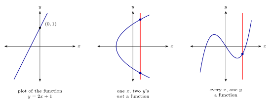
Worked: which of these is a function?
Let \(X = \{1,2,3\}\) and \(Y = \{1,2,3,4\}\). Which one of the following is a function from \(X\) to \(Y\)?
| Candidate | Why | ||
|---|---|---|---|
| (a) | \(\{(1,2), (1,3), (2,4)\}\) | ✗ | \(f(1) = 2\) and \(f(1) = 3\) — the value at \(1\) is not unique. (Also \(3\) is unused.) |
| (b) | \(\{(1,2), (2,3), (3,2), (4,1)\}\) | ✗ | \(4 \notin X\) — a pair whose first coordinate is outside the domain |
| (c) | \(\{(1,2), (2,3), (3,5)\}\) | ✗ | \(5 \notin Y\) — a value outside the codomain |
| (d) | \(\{(1,2), (2,1), (3,1)\}\) | ✓ | all first coordinates in \(X\), all second in \(Y\), each of \(1,2,3\) used exactly once |
Each wrong answer breaks a different one of the three conditions, which is what makes this a good question: the three failures are not variations on one mistake.
For (d): \(f(1) = 2\), \(f(2) = 1\), \(f(3) = 1\). Note \(f(2) = f(3)\) — two inputs sharing a value is not a problem, for exactly the reason the picture above shows.
Codomain and range
The two are constantly confused, and the difference is one word:
For a function \(f : X \to Y\), the co-domain is \(Y\), and the range is \(f(X) = \{f(x) : x \in X\}\), which is a subset of \(Y\).
| Is | Determined by | |
|---|---|---|
| Co-domain | \(Y\) — where values are allowed to land | the declaration \(f : X \to Y\) |
| Range | \(f(X)\) — where values actually land | the pairs in \(f\) |
So the codomain is a choice you make when you write down the function, and the range is a fact you compute. Always \(f(X) \subseteq Y\), and the containment is often proper.
For the function (d) above, \(f = \{(1,2),(2,1),(3,1)\}\):
\[\text{co-domain} = Y = \{1,2,3,4\} \qquad\qquad \text{range} = f(X) = \{1,2\} \subseteq Y\]
\(3\) and \(4\) are in the codomain and not in the range — they are permitted values that this particular function never takes.
Image and preimage
The two definitions generalise “range” to any subset, in each of the two directions:
If \(f : X \to Y\) is any function and \(A\) is any subset of \(X\), then the image of \(A\) is \[f(A) = \{f(x) : x \in A\}\]
If \(f : X \to Y\) is any function and \(B\) is any subset of \(Y\), then the inverse image or preimage of \(B\) is \[f^{-1}(B) = \{x \in X : f(x) \in B\}\]
Both take a set and return a set — \(A \subseteq X\) gives \(f(A) \subseteq Y\), and \(B \subseteq Y\) gives \(f^{-1}(B) \subseteq X\). The range is then just the image of the whole domain, \(f(X)\).
The notation \(f^{-1}\) here does not mean an inverse function. \(f^{-1}(B)\) is defined for any function, invertible or not — the emphasis on any in both definitions is the point. It is a set-to-set operation that always exists; an inverse function is a different thing that usually does not.
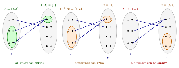
Figure 192: Image and preimage of the same function, read in opposite directions. Following the lines forward from a subset of X collects a subset of Y; following them backwards from a subset of Y collects every x that lands in it — which can be several elements, or none at all. In each panel the domain is on the left and the co-domain on the right, each line runs from an element of X to its value in Y, and the subset under discussion is outlined in colour with its expression in the same colour.
Worked
Let \(X = \{1,2,3\}\), \(Y = \{1,2,3,4\}\) and \(f = \{(1,2), (2,1), (3,1)\}\), the function from the question above. So \(f(1) = 2\), \(f(2) = 1\), \(f(3) = 1\).
| Asked for | Working | Answer | |
|---|---|---|---|
| (a) | image of \(\{1\}\) | \(f(1) = 2\) | \(f(\{1\}) = \{2\}\) |
| (b) | image of \(\{2,3\}\) | \(f(2) = 1\), \(f(3) = 1\) | \(f(\{2,3\}) = \{1\}\) |
| (c) | inverse image of \(\{2\}\) | which \(x\) have \(f(x) = 2\)? only \(x=1\) | \(f^{-1}(\{2\}) = \{1\}\) |
| (d) | preimage of \(\{1\}\) | which \(x\) have \(f(x) = 1\)? \(x = 2\) and \(x = 3\) | \(f^{-1}(\{1\}) = \{2,3\}\) |
| (e) | preimage of \(\{3,4\}\) | no \(x\) maps to \(3\) or \(4\) | \(f^{-1}(\{3,4\}) = \emptyset\) |
Three things this table is designed to show — they are the three panels of Figure 192:
- (b): an image can be smaller than the set you started with. \(\{2,3\}\) has two elements, \(f(\{2,3\})\) has one, because \(f\) sends both to the same place.
- (d): a preimage can be larger than the set you started with. One element of \(Y\) pulls back to two of \(X\).
- (e): a preimage can be empty. \(\{3,4\}\) lies outside the range entirely. Note this is a perfectly good answer, not a failure — \(\emptyset\) is a subset of \(X\) like any other, and it is the reason \(f^{-1}\) needs no invertibility to be defined.
Always write the answers as sets: \(f^{-1}(\{2\}) = \{1\}\), not \(= 1\). The operation returns a subset, and dropping the braces is the standard slip.
See also
- sets-and-set-notation — Cartesian products, and the \(\in\) / \(\subseteq\) distinction these definitions lean on
- proving-set-properties — the proof methods, for arguing about images and preimages
- relations-on-sets — functions as the relations with exactly one arrow out of each element
- 2026-09-03-set-properties-and-functions — Lecture 18
- practice-problems — §24 Functions Defined on General Sets, with full worked solutions
gcd, lcm & the Euclidean Algorithm
Greatest common divisor
For integers \(a\) and \(b\), not both zero, the greatest common divisor \(\gcd(a,b)\) is the integer \(d\) for which:
- \(d \mid a\) and \(d \mid b\) — \(d\) is a divisor of both; and
- \(\forall c \in \mathbb{Z}\), if \(c \mid a\) and \(c \mid b\) then \(c \leq d\) — every other common divisor is smaller.
Order doesn’t matter: \(\gcd(a,b) = \gcd(b,a)\).
On the name. \(\operatorname{hcf}(a,b)\) — highest common factor — names the same object; \(\gcd\) is the name this course uses.
Negatives. The divisors of \(15\) are \(1, 3, 5, 15, -1, -3, -5, -15\) — exactly the divisors of \(-15\). Since an integer and its negation have the same divisors, \(\gcd(-15, 36) = \gcd(15, 36)\), and in general
\[\gcd(a,b) = \gcd(|a|, |b|)\]
Note \(\gcd(0, b) = b\) for every positive integer \(b\) — this is the base case the Euclidean algorithm terminates on.
Lowest common multiple
For non-zero integers \(a\) and \(b\), the lowest common multiple \(\operatorname{lcm}(a,b)\) is the smallest integer \(n\) for which:
- \(n > 0\); and
- \(a \mid n\) and \(b \mid n\) — \(n\) is a multiple of both.
Again \(\operatorname{lcm}(a,b) = \operatorname{lcm}(b,a)\), and since the multiples of \(a\) are the multiples of \(-a\) (\(\dots, -10, -5, 0, 5, 10, 15, \dots\) for both \(5\) and \(-5\)),
\[\operatorname{lcm}(a,b) = \operatorname{lcm}(|a|, |b|)\]
Computing both from the prime factorisation
Using the standard factored form (see divisibility-and-factorisation): take the minimum exponent of each prime for the gcd, the maximum for the lcm.
\[30 = 2 \cdot 3 \cdot 5 \qquad 72 = 2^3 \cdot 3^2\] \[\gcd(30,72) = 2 \cdot 3 = 6 \qquad \operatorname{lcm}(30,72) = 2^3 \cdot 3^2 \cdot 5 = 360\]
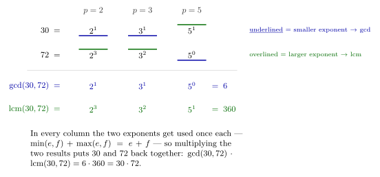
Figure 193: The min/max recipe laid out by prime column. In each column the blue underline marks the smaller exponent, which the gcd takes, and the green overline marks the larger, which the lcm takes. \(72\) has no factor of \(5\), so its entry in that column is \(5^0\). Setting it out this way also shows why the lemma \(\gcd \cdot \operatorname{lcm} = ab\) holds: in each column the smaller and larger exponents together are exactly the two original exponents.
Lemma: if \(a, b \in \mathbb{Z}^+\) then \[\gcd(a,b) \cdot \operatorname{lcm}(a,b) = ab\]
Checking: \(\gcd(30,72) \cdot \operatorname{lcm}(30,72) = 6 \cdot 360 = 2160 = 30 \cdot 72\). Each prime’s min and max exponents together account for both original exponents, which is why it works.
More generally, for non-zero integers \(a\) and \(b\): \(\gcd(a,b) \cdot \operatorname{lcm}(a,b) = |ab|\).
Worked
- \(\gcd(63, -105)\) and \(\operatorname{lcm}(63,-105)\): factor \(63 = 3^2 \cdot 7\) and \(-105 = -3 \cdot 5 \cdot 7\), then read off the common primes — \(\gcd = 3 \cdot 7 = 21\) and \(\operatorname{lcm} = 3^2 \cdot 5 \cdot 7 = 315\). (Keeping the minus sign out the front like this and replacing \(-105\) by \(105\) first both work, since \(\gcd(a,b) = \gcd(|a|,|b|)\).)
- For distinct primes \(p, q\): \(\gcd(p,q) = 1\) and \(\operatorname{lcm}(p,q) = pq\).
- \(\operatorname{lcm}(12,18)\): \(12 = 2^2 \cdot 3\), \(18 = 2 \cdot 3^2\), so \(\operatorname{lcm} = 2^2 \cdot 3^2 = 36\).
- \(\operatorname{lcm}(2^2 \cdot 3 \cdot 5,\; 2^3 \cdot 3^2) = 2^3 \cdot 3^2 \cdot 5 = 360\).
- \(\operatorname{lcm}(2800, 6125)\): \(2800 = 2^4 \cdot 5^2 \cdot 7\) and \(6125 = 5^3 \cdot 7^2\), so \(\operatorname{lcm} = 2^4 \cdot 5^3 \cdot 7^2 = 98\,000\).
The Euclidean algorithm
Factorising large numbers is slow; the Euclidean algorithm finds \(\gcd(a,b)\) for \(a, b \in \mathbb{Z}^+\) without it. It rests on this fact:
If \(a, b \in \mathbb{Z}\) are not both zero and \(q, r \in \mathbb{Z}\) satisfy \(a = bq + r\), then \(\gcd(a,b) = \gcd(b,r)\).
Why: suppose \(c \mid a\) and \(c \mid b\); then \(c \mid (a - bq)\) and hence \(c \mid r\). Conversely suppose \(d \mid b\) and \(d \mid r\); then \(d \mid (bq + r)\) and hence \(d \mid a\). So the two pairs have exactly the same common divisors, and therefore the same greatest one.
The method: divide the bigger by the smaller, keep the remainder, repeat — the pair shrinks each round until the remainder is 0, and then \(\gcd(x, 0) = x\).
\(\gcd(5859, 1232)\):
| Division | Consequence |
|---|---|
| \(5859 = 1232 \cdot 4 + 931\) | \(\gcd(5859,1232) = \gcd(1232,931)\) |
| \(1232 = 931 \cdot 1 + 301\) | \(\gcd(1232,931) = \gcd(931,301)\) |
| \(931 = 301 \cdot 3 + 28\) | \(\gcd(931,301) = \gcd(301,28)\) |
| \(301 = 28 \cdot 10 + 21\) | \(\gcd(301,28) = \gcd(28,21)\) |
| \(28 = 21 \cdot 1 + 7\) | \(\gcd(28,21) = \gcd(21,7)\) |
| \(21 = 7 \cdot 3 + 0\) | \(\gcd(21,7) = \gcd(7,0) = 7\) |
So \(\gcd(5859, 1232) = 7\).
\(\gcd(4131, 2431)\):
\[4131 = 2431 \cdot 1 + 1700, \quad 2431 = 1700 \cdot 1 + 731, \quad 1700 = 731 \cdot 2 + 238,\] \[731 = 238 \cdot 3 + 17, \quad 238 = 17 \cdot 14 + 0\]
so \(\gcd(4131,2431) = \gcd(17,0) = 17\).
\(\gcd(14, 3003)\): \(3003 = 14 \cdot 214 + 7\), then \(14 = 7 \cdot 2 + 0\), so the gcd is \(7\).
\(\gcd(931, 301)\): \(931 = 301 \cdot 3 + 28\), \(301 = 28 \cdot 10 + 21\), \(28 = 21 \cdot 1 + 7\), \(21 = 7 \cdot 3 + 0\), so \(\gcd = 7\). Using that, \(7 \mid 931\) and \(931 = 7 \cdot 133 = 7 \cdot 7 \cdot 19 = 7^2 \cdot 19\), which has \((2+1)(1+1) = 6\) positive divisors.
\(\gcd(116, 88)\): \(116 = 88 \cdot 1 + 28\), \(88 = 28 \cdot 3 + 4\), \(28 = 4 \cdot 7 + 0\), so \(\gcd = 4\); hence \(\operatorname{lcm}(116,88) = \frac{116 \cdot 88}{4} = 2552\).
As pseudocode
Input: A, B (integers with A > B >= 0)
a := A; b := B; r := B
while b != 0:
    r := a mod b
    a := b
    b := r
gcd := a
Output: gcd
Trace table for \(A = 1001\), \(B = 871\):
| 0 | 1 | 2 | 3 | 4 | 5 | |
|---|---|---|---|---|---|---|
| \(a\) | 1001 | 871 | 130 | 91 | 39 | 13 |
| \(b\) | 871 | 130 | 91 | 39 | 13 | 0 |
| \(r\) | 871 | 130 | 91 | 39 | 13 | 0 |
| gcd | 13 |
Proofs about gcd and lcm
For all positive integers \(a\) and \(b\), \(a \mid b\) if and only if \(\operatorname{lcm}(a,b) = b\).
A biconditional can be proved either way round, but proving each direction separately is the recommended method — proving both simultaneously by chaining “iff”s is quicker but easy to get logically wrong (every link in the chain must genuinely be reversible).
(\(\Rightarrow\)) Suppose \(a, b \in \mathbb{Z}^+\) and \(a \mid b\). Then \(b = ka\) for some \(k \in \mathbb{Z}\). So \(\operatorname{lcm}(a,b) = \operatorname{lcm}(a, ka)\). Since \(a \mid ka\) and \(ka \mid ka\), and no smaller \(n > 0\) has \(ka \mid n\), we get \(\operatorname{lcm}(a, ka) = ka = b\).
(\(\Leftarrow\)) Suppose \(\operatorname{lcm}(a,b) = b\). By the definition of lcm, \(a \mid \operatorname{lcm}(a,b)\); substituting the hypothesis gives \(a \mid b\). \(\square\)
For all positive integers \(a\) and \(b\), \(\gcd(a,b) = \operatorname{lcm}(a,b)\) if and only if \(a = b\).
(\(\Leftarrow\)) If \(a = b\) then both equal \(a\).
(\(\Rightarrow\)) Assume \(\gcd(a,b) = \operatorname{lcm}(a,b)\) and set \(g = \gcd(a,b)\), so \(a = gm\) and \(b = gn\) for positive integers \(m, n\) with \(\gcd(m,n) = 1\). Since \(gm\) and \(gn\) share no prime factors beyond those in \(g\), the lcm uses all primes from both: \(\operatorname{lcm}(a,b) = gmn\). From \(g = gmn\) we get \(mn = 1\), so \(m = n = 1\) and \(a = b = g\). \(\square\)
Extended Euclidean algorithm (non-assessed)
Theorem: for \(a, b, c \in \mathbb{Z}\), if \(\gcd(a,b) \mid c\) then there exist integers \(x\) and \(y\) with \(ax + by = c\).
Running the Euclidean algorithm’s steps in reverse finds them. For \(1232x + 5859y = 14\):
- Run the algorithm (as above) to get \(\gcd(1232, 5859) = 7\).
- Work backwards from the second-last equation, substituting each remainder in turn:
\[7 = 28 - 21\] \[= 28 - (301 - 28 \cdot 10) = 28 \cdot 11 - 301\] \[= (931 - 301 \cdot 3) \cdot 11 - 301 = 931 \cdot 11 - 301 \cdot 34\] \[= 931 \cdot 45 - 1232 \cdot 34\] \[= (5859 - 1232 \cdot 4) \cdot 45 - 1232 \cdot 34 = 5859 \cdot 45 - 1232 \cdot 214\]
- Scale to the target: \(7 = 1232(-214) + 5859(45)\), so \(14 = 1232(-428) + 5859(90)\).
This content is not examinable, but it’s where gcd earns its keep in practice. It is used to determine whether certain types of equations have solutions (the linear Diophantine equations \(ax + by = c\)), and it has applications in cryptography (the modular inverses this same reversal computes).
Where this gets used
Adding fractions and other everyday arithmetic; deciding whether certain equations have integer solutions; applications in cryptography.
See also
- divisibility-and-factorisation · modular-arithmetic · proof-techniques
- integers-modulo-n — multiplicative inverses mod \(p\), found there by search, which the reversed algorithm also computes
- inclusion-exclusion — divisible by both \(a\) and \(b\) means divisible by \(\operatorname{lcm}(a, b)\), the step that counts the overlaps of sets of multiples
- practice-problems — §15 The Euclidean Algorithm, with full worked solutions
Graphs
A graph is a set of points, the vertices, with some of them joined by lines, the edges. Almost all of graph theory is built on the few definitions here: what a graph is, loops and multiple edges, simple graphs, and the degree of a vertex. Then the first theorem, the Handshake Theorem, which says the degrees always add up to twice the number of edges, and what follows from it: every graph has an even number of vertices of odd degree, and many lists of numbers cannot be the degrees of any graph. The pigeonhole argument that two vertices of a simple graph share a degree is in pigeonhole-principle. First met in 2026-10-22-pigeonhole-principle-introduction-to-graph-theory. What comes after builds on these: getting around a graph (walks-trails-and-circuits), using every edge exactly once (euler-circuits-and-trails), writing a graph as a matrix (adjacency-matrices, incidence-matrices), and the connected graphs with no circuits ([trees]).
What a graph is
A graph \(G\) is a non-empty set of vertices \(V(G)\) and a (possibly empty) set of edges \(E(G)\), where each edge is associated with a set consisting of either one or two vertices.
The vertices an edge is associated with are its endpoints. An edge with two endpoints joins them, and an edge with one endpoint joins that vertex to itself.
- A graph must have at least one vertex, but it may have no edges at all.
- An edge is an object in its own right, not just a pair of vertices. Two different edges can have the same endpoints, and that is why edges are given their own names, \(e_1, e_2, \dots\).
Two standard words: two vertices joined by an edge are adjacent, and an edge is incident with each of its endpoints. A vertex with no edges at all is isolated.
Drawing a graph. Each vertex is a dot and each edge a line between the dots of its endpoints, or a small loop from a dot back to itself. The graph is only the vertices, the edges and which edges have which endpoints. Where the dots go, and whether the lines are straight or curved, carry no information, so the same graph can be drawn in many ways. Two lines that cross in a drawing do not meet at a vertex; only dots are vertices.
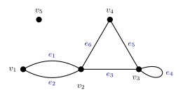
Figure 194: A graph with vertices \(v_1\) to \(v_5\) and edges \(e_1\) to \(e_6\). The edges \(e_1\) and \(e_2\) have the same endpoints, \(v_1\) and \(v_2\), so they are multiple edges. The edge \(e_4\) has the single endpoint \(v_3\), so it is a loop. \(v_5\) is an isolated vertex: no edge has it as an endpoint, but it is still part of the graph. The edge \(e_6\) joins \(v_2\) and \(v_4\), so those two vertices are adjacent and \(e_6\) is incident with each of them; \(v_1\) and \(v_3\) are not adjacent, since no edge joins them. The graph is not simple, because of the loop and because of the multiple edges.
| Edge | Endpoints |
|---|---|
| \(e_1\) | \(\{v_1, v_2\}\) |
| \(e_2\) | \(\{v_1, v_2\}\) |
| \(e_3\) | \(\{v_2, v_3\}\) |
| \(e_4\) | \(\{v_3\}\) |
| \(e_5\) | \(\{v_3, v_4\}\) |
| \(e_6\) | \(\{v_2, v_4\}\) |
The table is the graph. The drawing is one picture of it.
Loops and multiple edges
- A loop is an edge with only one endpoint. It joins a vertex to itself. Above, \(e_4\) is a loop at \(v_3\).
- Multiple edges (also called parallel edges) are two or more edges with the same set of endpoints. Above, \(e_1\) and \(e_2\) both join \(v_1\) and \(v_2\).
Both come up naturally when a graph models something. In the bridges of Königsberg, two land masses are joined by two bridges, which gives multiple edges (2026-07-27-welcome-and-intro-problems).
Simple graphs
A graph is simple if it has no loops and no multiple edges.
In a simple graph every edge has two different endpoints, and two vertices are joined by at most one edge. So an edge can be named by its endpoints, and a simple graph is just a set of vertices with some pairs of them joined.
A simple graph with \(n\) vertices has every degree at most \(n - 1\). A vertex can be joined to each of the other \(n - 1\) vertices at most once, and not to itself. This bound is one of the two quick tests for degree sequences.
Degree
The degree of a vertex \(v\), written \(\deg(v)\), is the number of edge ends incident with it.
Count the ends of edges at the vertex, not the edges.
- An ordinary edge has one end at each of its two endpoints, so it adds 1 to the degree of each.
- A loop has both of its ends at the same vertex, so it adds 2 to the degree of that vertex.
- An isolated vertex has degree 0.
In the graph above:
| Vertex | Edge ends at it | Degree |
|---|---|---|
| \(v_1\) | \(e_1\), \(e_2\) | 2 |
| \(v_2\) | \(e_1\), \(e_2\), \(e_3\), \(e_6\) | 4 |
| \(v_3\) | \(e_3\), \(e_4\) twice, \(e_5\) | 4 |
| \(v_4\) | \(e_5\), \(e_6\) | 2 |
| \(v_5\) | none | 0 |
The degrees add to \(2 + 4 + 4 + 2 + 0 = 12\), and there are 6 edges.
Why a loop counts 2: degree counts the ways out of a vertex along an edge. A loop can be set off along in either direction, so it gives two ways out. Counting it as 2 is also what makes the Handshake Theorem hold for every graph.
The Handshake Theorem
The Handshake Theorem. The sum of the degrees of a graph is twice the number of edges. If \(G\) is a graph with \(V(G) = \{v_1, v_2, \dots, v_n\}\) and \(|E(G)| = e\), then \[\sum_{i=1}^{n} \deg(v_i) = \deg(v_1) + \deg(v_2) + \cdots + \deg(v_n) = 2e.\]
Proof. Count the edge ends in the graph two ways. Every edge has exactly two ends: an edge with two endpoints has one at each, and a loop has both at its one endpoint. So there are \(2e\) ends in all. Every end is at exactly one vertex, and \(\deg(v_i)\) is the number of ends at \(v_i\). So adding the degrees over all the vertices counts each end exactly once, and the sum is \(2e\). \(\square\)
The name comes from people shaking hands at a party. Each handshake involves two hands, so the total number of hands shaken, added up person by person, is twice the number of handshakes.
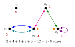
Figure 195: The proof of the Handshake Theorem, on the graph above. Every edge is drawn in its own colour, with a dot of that colour at each of its two ends. The loop \(e_4\) has both of its dots at \(v_3\). The degree of a vertex is the number of dots at it, so adding up the degrees counts every dot once. Each edge has exactly two dots, so the 6 edges give 12 dots, and the degrees add to 12.
Using it. The theorem links the degrees to the number of edges, so either can be found from the other.
- Number of edges from the degrees. A graph with degrees \(4, 4, 3, 3, 2, 2\) has \(\frac{18}{2} = 9\) edges.
- No graph with an odd degree sum. There is no graph with 7 vertices each of degree 3: the degrees would add to 21, and 21 is not \(2e\) for any whole number \(e\). More generally, if every vertex has degree 3 then \(3n = 2e\), so the number of vertices \(n\) must be even.
- Edges of a complete graph, below.
Odd-degree vertices come in pairs
Corollary. Every graph has an even number of vertices of odd degree.
Proof. Split the sum of the degrees into the vertices of even degree and the vertices of odd degree:
\[\underbrace{\sum_{\deg(v) \text{ even}} \deg(v)}_{\text{even}} \;+\; \sum_{\deg(v) \text{ odd}} \deg(v) \;=\; 2e.\]
The first sum is a sum of even numbers, so it is even. The right side is even. So the second sum, being the difference of two even numbers, is even. It is a sum of odd numbers, and a sum of odd numbers is even exactly when there is an even number of terms: odd numbers pair up into even sums, and one left over makes the total odd. So the number of vertices of odd degree is even. \(\square\)
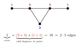
Figure 196: The corollary on a graph with degrees 3, 3, 2, 1, 1, odd degrees in red and even in blue. The degree sum is \(2e = 10\), even. Its even part, 2, is even, so its odd part, \(3 + 3 + 1 + 1\), must be even as well. A sum of odd numbers is even only when the odd numbers pair off, each pair adding to an even number. Here the four odd degrees make two pairs. A fifth vertex of odd degree would be left without a partner and make the total odd, which no graph allows.
The corollary says nothing about the vertices of even degree. Their number can be odd or even: one vertex joined to four others has one vertex of even degree, and a path of four vertices has two. That is worked as a multiple-choice question in 2026-10-22-pigeonhole-principle-introduction-to-graph-theory.
In practice the corollary is the quickest check on a list of degrees: count the odd entries. If there is an odd number of them, no graph has those degrees.
Degree sequences
The list of the degrees of the vertices in a graph is called the degree sequence of the graph.
It is usually written largest first. The graph above has degree sequence \(4, 4, 2, 2, 0\). Only the list of numbers matters, not which vertex has which.
The usual question runs the other way: given a list, is there a graph, often a simple graph, with exactly those degrees? Two checks rule a list out:
- The sum must be even, by the Handshake Theorem. Equivalently, the number of odd entries must be even. This holds for every graph.
- For a simple graph with \(n\) vertices, no entry can be more than \(n - 1\). A list of \(n\) numbers with an entry of \(n\) or more has no simple graph.
These checks are necessary, not sufficient. A list can pass both and still have no simple graph. Take \(3, 3, 3, 1\). The sum is 10, which is even, and no entry is more than \(n - 1 = 3\). But with 4 vertices, a vertex of degree 3 in a simple graph is joined to all three others. There are three such vertices, and each of them is joined to the fourth vertex, which therefore has degree 3, not 1. So no simple graph has degree sequence \(3, 3, 3, 1\).
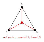
Figure 197: Why no simple graph has degree sequence 3, 3, 3, 1. In a simple graph on 4 vertices, a vertex of degree 3 is joined to every other vertex. The three vertices that need degree 3, black, must each be joined to the fourth vertex, red, which is then forced to have degree 3 as well. The list passes both quick checks, an even sum and no degree above 3, and still has no simple graph.
So, after the two checks, a list that passes either gets a drawing or an argument like this one. Small cases can be settled by hand, building the graph from the vertex of largest degree down. A complete test for when a list is the degree sequence of a simple graph does exist (the Havel–Hakimi and Erdős–Gallai theorems), but it is beyond this course.
Without the word “simple”, the answer is easy. If loops are allowed, every list with an even sum is the degree sequence of some graph. The odd entries come in an even number, so pair them up and join each pair by an edge. Now every vertex still needs an even number of edge ends, and a loop supplies 2, so add loops until each vertex has its degree. For example, \(3, 2, 1\) has no simple graph, since degree 3 is impossible with only 3 vertices, but a graph with multiple edges has those degrees (2026-10-22-pigeonhole-principle-introduction-to-graph-theory).
Worked: which lists are degree sequences
For each list, is there a simple graph with those degrees?
| List | Sum | Largest vs \(n - 1\) | Simple graph? |
|---|---|---|---|
| \(2, 2, 2, 2\) | 8 | \(2 \le 3\) | yes: a square |
| \(3, 2, 1\) | 6 | \(3 > 2\) | no: too large |
| \(4, 3, 2, 2, 2, 2, 1, 1\) | 17 | \(4 \le 7\) | no: odd sum (three odd entries) |
| \(1, 1, 1, 1\) | 4 | \(1 \le 3\) | yes: two edges with no common vertex |
| \(5, 5, 5, 5, 5, 5\) | 30 | \(5 \le 5\) | yes: the complete graph \(K_6\) |
| \(3, 3, 3, 1\) | 10 | \(3 \le 3\) | no: passes both checks, fails as shown |
| \(4, 4, 3, 3, 2, 2\) | 18 | \(4 \le 5\) | yes: 9 edges |
The first five are drawn in 2026-10-22-pigeonhole-principle-introduction-to-graph-theory. For the last, name the vertices \(a, b, c, d, e, f\) with the degrees in that order, and take the edges \(ac, ad, ae, af, bc, bd, be, bf, cd\). Then \(a\) and \(b\) are each joined to \(c, d, e, f\); \(c\) and \(d\) to \(a\), \(b\) and each other; and \(e\) and \(f\) to \(a\) and \(b\).
Complete graphs
The complete graph \(K_n\) is the simple graph with \(n\) vertices in which every pair of different vertices is joined by an edge. It is the standard name for this graph. Every vertex is joined to the other \(n - 1\), so every degree is \(n - 1\), the most a simple graph allows. \(K_6\) is the graph with degree sequence \(5, 5, 5, 5, 5, 5\).
How many edges? By the Handshake Theorem,
\[n(n - 1) = 2e, \qquad\text{so}\qquad e = \frac{n(n-1)}{2}.\]
Or count directly: an edge of \(K_n\) is a choice of 2 of the \(n\) vertices, so there are \(\binom{n}{2} = \frac{n(n-1)}{2}\) edges (counting-selections). The two counts agree. \(K_6\) has \(\frac{6 \cdot 5}{2} = 15\) edges.
\(\binom{n}{2}\) is the most edges a simple graph on \(n\) vertices can have. Each edge of a simple graph is a different pair of vertices, and there are only \(\binom{n}{2}\) pairs. \(K_n\) uses every pair, so it is the only simple graph on \(n\) vertices that reaches the bound.
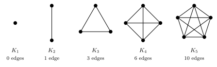
Figure 198: The complete graphs \(K_1\) to \(K_5\), each with every pair of vertices joined. Each vertex of \(K_n\) has degree \(n - 1\), so the degrees add to \(n(n-1)\) and there are \(\frac{n(n-1)}{2}\) edges: 0, 1, 3, 6 and 10. In \(K_4\) and \(K_5\) some lines cross where there is no vertex. Only the dots are vertices.
Common mistakes
- Counting a loop once. A loop adds 2 to the degree of its vertex. Counting it as 1 makes the degree sum odd and breaks the Handshake Theorem.
- Treating a crossing as a vertex. Lines that cross in a drawing are not joined. A vertex is a dot.
- Taking an even sum as enough. The Handshake Theorem rules a list out when its sum is odd, but an even sum does not make a simple graph exist: \(3, 2, 1\) and \(3, 3, 3, 1\) both have even sums and no simple graph.
- Forgetting the word “simple”. Without it, loops and multiple edges are allowed, and any list with an even sum has a graph. With it, every degree is at most \(n - 1\).
- Mixing up the corollary. The number of vertices of odd degree is always even. The number of vertices of even degree can be anything.
- Reading the drawing as the graph. Where the dots are and how the lines bend do not matter. The graph is the vertices, the edges and their endpoints.
See also
- pigeonhole-principle — every simple graph with at least two vertices has two vertices of equal degree
- counting-selections — \(\binom{n}{2}\), the number of edges of \(K_n\)
- 2026-07-27-welcome-and-intro-problems — the bridges of Königsberg as a graph
- walks-trails-and-circuits — walks, trails, circuits and connected graphs
- euler-circuits-and-trails — when a graph can be traced using every edge exactly once
- adjacency-matrices · incidence-matrices — a graph written as a matrix
- [trees] — connected graphs with no circuits
- 2026-10-22-pigeonhole-principle-introduction-to-graph-theory — Lecture 33
- 2026-10-26-walks-trails-and-circuits — Lecture 34, which recaps these definitions
- practice-problems — §43, with full worked solutions
Groups
A group is a set together with one operation on it that satisfies four properties: closure, associativity, identity and inverses. The four are enough to solve any equation \(a * x = b\). The course’s examples are numbers under addition, non-zero real numbers under multiplication, the classes of integers-modulo-n, and the bijections of the symmetric-group under composition. A small group is checked from its table (cayley-tables). Groups inside groups, and the powers of an element, are in subgroups-and-cyclic-groups. First met in 2026-09-24-definitions-and-examples-of-groups, and continued in 2026-10-06-elementary-properties-of-groups.
The definition
Definition: If \(G\) is a set and \(*\) is a binary operation on \(G\), then \((G, *)\) is a group if it has the following properties:-
(1) Closure: for all \(g, h \in G\), \(g * h \in G\).
(2) Associativity: for all \(g, h, k \in G\), \((g * h) * k = g * (h * k)\).
(3) Identity: \(\exists e \in G\) such that \(\forall g \in G\), \(e * g = g * e = g\).
(4) Inverses: \(\forall g \in G\), \(\exists g^{-1} \in G\) such that \(g * g^{-1} = g^{-1} * g = e\).
A binary operation combines two elements, taken in order, into one result. Addition and multiplication of numbers are binary operations, and so is composition of functions.
| Property | In words |
|---|---|
| closure | Combining two elements of \(G\) gives an element of \(G\). The operation never leaves the set. |
| associativity | Three elements in a row can be bracketed either way. |
| identity | One element, \(e\), changes nothing when combined with anything, on either side. |
| inverses | Every element has a partner in \(G\) that takes it back to \(e\), on either side. |
Points that are easy to read past:
- A group is the pair. The set alone is not a group, and neither is the operation. \((\mathbb{Z}, +)\) is a group and \((\mathbb{Z}, -)\) is not. They have the same set.
- Both sides. The identity must satisfy \(e * g = g\) and \(g * e = g\). An inverse must work on both sides too.
- The order of the quantifiers. Property (3) is \(\exists e\, \forall g\): a single \(e\) that works for every \(g\). Property (4) is \(\forall g\, \exists g^{-1}\): each \(g\) has its own inverse (quantified-statements).
- \(g^{-1}\) is notation for “the inverse of \(g\) in this group”. In \((\mathbb{R}, +)\), \(x^{-1} = -x\). It is a reciprocal only when the operation is multiplication.
- The inverse must be in \(G\). In \((\mathbb{Z} - \{0\}, \cdot)\) the equation \(2 \cdot y = 1\) has the solution \(\frac12\), which is not in the set. So 2 has no inverse there.
Commutative and abelian
A binary operation \(*\) on \(S\) is commutative if \(a * b = b * a\) for all \(a, b \in S\). A group is abelian if and only if its operation is commutative.
Commutativity is not one of the four properties. A group may or may not have it.
| abelian | \((\mathbb{Z}, +)\), \((\mathbb{R}, +)\), \((\mathbb{R} - \{0\}, \cdot)\), \((\mathbb{Z}_n, +)\), \((\mathbb{Z}_7 - \{[0]\}, \cdot)\) |
| non-abelian | \((S_3, \circ)\): \(f_2 \circ f_3 = f_6\) but \(f_3 \circ f_2 = f_5\) |
| \((F, \circ)\), the functions \(ax + b\) with \(a \neq 0\) (below): with \(f(x) = 2x\) and \(g(x) = x + 1\), \((f \circ g)(x) = 2x + 2\) but \((g \circ f)(x) = 2x + 1\) |
In a group that is not known to be abelian, keep the order of every product, and do the same thing on the same side of both sides of an equation. To show a group is not abelian, one pair with \(a * b \neq b * a\) is enough (2026-09-24-definitions-and-examples-of-groups).
Associativity is about brackets, not order
Associativity says \((g * h) * k = g * (h * k)\). The three elements stay in the same order, and only the bracketing changes. It is what allows \(g * h * k\) to be written with no brackets at all. It says nothing about swapping elements, which is commutativity.
Subtraction on \(\mathbb{Z}\) is an operation that is not associative: \((3 - 2) - 1 = 0\) but \(3 - (2 - 1) = 2\). The figure sets it beside addition, which is.
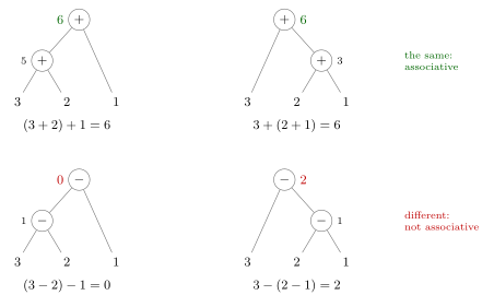
Figure 199: The two ways of bracketing three elements, drawn as trees: the lower operation is done first, and its result feeds the upper one. Top row, addition: both bracketings of \(3 + 2 + 1\) give 6. Addition is associative, so the brackets can be dropped. Bottom row, subtraction: \((3 - 2) - 1 = 0\) and \(3 - (2 - 1) = 2\). The same three numbers in the same order give different answers, so subtraction is not associative and \((\mathbb{Z}, -)\) is not a group.
| Operation | Associative | Commutative |
|---|---|---|
| \(+\) and \(\cdot\) on numbers | yes | yes |
| \(\circ\) on functions | yes | no |
| \(-\) on \(\mathbb{Z}\) | no | no |
Checking the four properties
Each property is a quantified statement, so each is proved in general and disproved with specific elements.
| Property | To show it holds | To show it fails |
|---|---|---|
| closure | Take arbitrary \(g, h \in G\) and show \(g * h \in G\). | Two elements of \(G\) whose result is outside \(G\). |
| associativity | Usually inherited: the operation is built from addition or multiplication of numbers, or is composition of functions. Otherwise compute both bracketings for arbitrary \(g, h, k\). | Three elements whose two bracketings differ. |
| identity | Name \(e\), check \(e \in G\), and check \(e * g = g\) and \(g * e = g\) for arbitrary \(g\). | Show that no element can do the job. |
| inverses | For arbitrary \(g\), name \(g^{-1}\), check it is in \(G\), and check both products are \(e\). | One element of \(G\) with no inverse in \(G\). |
Do identity before inverses, since inverses are defined in terms of \(e\). When \(e\) or \(g^{-1}\) is not obvious, solve for it: write down the equation it has to satisfy and solve.
Worked: an unfamiliar operation
From practice-problems, Q2. Let \(G\) be the set of odd integers, with \(x \star y = x + y - 1\).
- Closure. If \(x, y\) are odd then \(x + y\) is even, so \(x + y - 1\) is odd.
- Associativity. \((x \star y) \star z = (x + y - 1) + z - 1 = x + y + z - 2\), and \(x \star (y \star z) = x + (y + z - 1) - 1 = x + y + z - 2\).
- Identity. Solve \(x \star e = x\): \(x + e - 1 = x\) gives \(e = 1\), which is odd. Check the other side: \(1 \star x = 1 + x - 1 = x\).
- Inverses. Solve \(x \star y = 1\): \(x + y - 1 = 1\) gives \(y = 2 - x\), which is odd when \(x\) is. So \(x^{-1} = 2 - x\).
It is also commutative, since \(x + y - 1 = y + x - 1\), so \((G, \star)\) is an abelian group. The identity is 1, not 0, and the inverse of \(x\) is \(2 - x\), not \(-x\). They are whatever the operation makes them.
Eight candidates
Which of these eight pairs are groups (2026-09-24-definitions-and-examples-of-groups)? All eight against all four properties:
| Closure | Associative | Identity | Inverses | Group? | |
|---|---|---|---|---|---|
| \((\mathbb{Z}, +)\) | \(\checkmark\) | \(\checkmark\) | \(0\) | \(-x\) | yes |
| \((\mathbb{Z} - \{0\}, \cdot)\) | \(\checkmark\) | \(\checkmark\) | \(1\) | \(\times\) 2 has none | no |
| \((\mathbb{Z}, -)\) | \(\checkmark\) | \(\times\) \((3-2)-1 \neq 3-(2-1)\) | \(\times\) | — | no |
| \((\mathbb{Z}_3, +)\) | \(\checkmark\) | \(\checkmark\) | \([0]\) | \([-a]\) | yes |
| \((\mathbb{Z}_5 - \{[0]\}, \cdot)\) | \(\checkmark\) | \(\checkmark\) | \([1]\) | \(\checkmark\) | yes |
| \((\mathbb{R}, +)\) | \(\checkmark\) | \(\checkmark\) | \(0\) | \(-x\) | yes |
| \((\mathbb{R}, \cdot)\) | \(\checkmark\) | \(\checkmark\) | \(1\) | \(\times\) 0 has none | no |
| \((\mathbb{R} - \{0\}, \cdot)\) | \(\checkmark\) | \(\checkmark\) | \(1\) | \(\frac1x\) | yes |
Some of the entries need a word:
- \((\mathbb{Z} - \{0\}, \cdot)\). Closed, associative, identity 1. Only 1 and \(-1\) have inverses in the set.
- \((\mathbb{Z}, -)\). As well as failing associativity it has no identity. \(g - e = g\) forces \(e = 0\), but \(0 - g = -g\), which is not \(g\) unless \(g = 0\). So 0 works on the right only.
- \((\mathbb{R}, \cdot)\) and \((\mathbb{R} - \{0\}, \cdot)\). The only obstacle is 0, since \(0 \cdot y = 1\) has no solution. Removing it leaves a set that is still closed, because a product of non-zero reals is non-zero.
- \((\mathbb{Z}_5 - \{[0]\}, \cdot)\). Its table is Q4 of practice-problems: \([1]^{-1} = [1]\), \([2]^{-1} = [3]\), \([3]^{-1} = [2]\), \([4]^{-1} = [4]\).
Removing elements can also break closure. \(\mathbb{Z}_9 - \{[0]\}\) is not a group under multiplication, because \([3] \cdot [3] = [0]\) is not in the set (the same practice set, Q1, which writes the classes without brackets). See integers-modulo-n.
A group of functions: \(ax + b\)
Let \(F\) be the set of all functions \(f(x) = ax + b\) with \(a \in \mathbb{R} - \{0\}\) and \(b \in \mathbb{R}\). Under composition, \((F, \circ)\) is a group (2026-10-06-elementary-properties-of-groups). Every check works the same way: compose, collect into the form \((\text{number})\,x + (\text{number})\), and read off the coefficients.
| Property | For \(f(x) = ax + b\) and \(g(x) = cx + d\) |
|---|---|
| closure | \((f \circ g)(x) = (ac)\,x + (ad + b)\), and \(ac \neq 0\) because \(a, c \neq 0\) |
| associativity | composition of functions is always associative (above) |
| identity | \(I(x) = x\), found by solving \(I \circ f = f\) for the coefficients of \(I\) |
| inverses | \(f^{-1}(x) = \frac1a x - \frac{b}{a}\), found by solving \(f \circ g = I\) for \(c\) and \(d\), then checked in the other order |
The condition \(a \neq 0\) is what keeps the inverses: a constant function \(0x + b\) sends everything to \(b\), and nothing undoes that. It is also a second non-abelian group, after \(S_3\), since \(f \circ g\) and \(g \circ f\) have constants \(ad + b\) and \(cb + d\), which usually differ.
Why these four: solving equations
Solving \(2x = 4\) means applying an inverse to both sides:
\[2x = 4, \qquad 2^{-1} \cdot 2x = 2^{-1} \cdot 4, \qquad x = 2.\]
The same steps solve \(a * x = b\) in any group, and each step uses one property:
\[\begin{aligned} a * x &= b \\ a^{-1} * (a * x) &= a^{-1} * b && a^{-1} \text{ exists, by inverses} \\ (a^{-1} * a) * x &= a^{-1} * b && \text{by associativity} \\ e * x &= a^{-1} * b && \text{by inverses} \\ x &= a^{-1} * b && \text{by identity} \end{aligned}\]
The working shows that a solution can only be \(a^{-1} * b\), and closure says that element is in \(G\). It is a solution: \(a * (a^{-1} * b) = (a * a^{-1}) * b = e * b = b\). So in a group every equation \(a * x = b\) has exactly one solution.
Two consequences:
- Cancellation. If \(a * b = a * c\) then \(b = c\): apply \(a^{-1}\) on the left of both sides. It is why a Cayley table has no repeats in a row (cayley-tables, proved in 2026-09-24-definitions-and-examples-of-groups).
- Sides matter. \(a^{-1}\) went on the left of both sides because \(a\) was on the left. For \(x * a = b\) it goes on the right, giving \(x = b * a^{-1}\). In a non-abelian group \(a^{-1} * b\) and \(b * a^{-1}\) can differ.
Without inverses an equation can have no solution. In \((\mathbb{Z} - \{0\}, \cdot)\), \(2x = 3\) has none, because 2 has no inverse.
Elementary properties
A handful of facts follow from the four properties alone, so they hold in every group. They are what justify writing the identity and the inverse.
The identity is unique. Suppose \(e\) and \(e'\) are both identities. Then
\[e = e * e' = e',\]
the first step because \(e'\) is an identity and the second because \(e\) is.
Each element has exactly one inverse. Suppose \(h\) and \(k\) are both inverses of \(g\). Then
\[h = h * e = h * (g * k) = (h * g) * k = e * k = k,\]
using identity, \(k\) an inverse, associativity, \(h\) an inverse, and identity. So to show that some \(x\) is \(g^{-1}\), it is enough to show \(g * x = x * g = e\).
The inverse of an inverse. \(g * g^{-1} = g^{-1} * g = e\) says, read the other way round, that \(g\) is an inverse of \(g^{-1}\). By uniqueness,
\[(g^{-1})^{-1} = g.\]
Equivalently, if \(g^{-1} = h\) then \(h^{-1} = g\). Inverses come in pairs, or an element is its own inverse, as the three swaps in \(S_3\) are.
The inverse of a product reverses the order.
\[(g * h)^{-1} = h^{-1} * g^{-1}.\]
Check both products, using associativity to regroup:
\[(g * h) * (h^{-1} * g^{-1}) = g * (h * h^{-1}) * g^{-1} = g * e * g^{-1} = g * g^{-1} = e,\]
\[(h^{-1} * g^{-1}) * (g * h) = h^{-1} * (g^{-1} * g) * h = h^{-1} * e * h = h^{-1} * h = e.\]
By uniqueness, \(h^{-1} * g^{-1}\) is the inverse of \(g * h\). The last thing done is the first thing undone, as with putting on socks and then shoes.
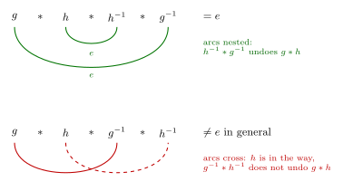
Figure 200: Why the inverse of \(g * h\) is \(h^{-1} * g^{-1}\) and not \(g^{-1} * h^{-1}\). Top: in \(g * h * h^{-1} * g^{-1}\) each element sits next to its inverse once the inner pair is gone. The inner arc, \(h * h^{-1} = e\), cancels first, and that brings \(g\) next to \(g^{-1}\), so the whole product is \(e\). The arcs are nested. Bottom: in \(g * h * g^{-1} * h^{-1}\) the arcs cross. \(h\) sits between \(g\) and \(g^{-1}\), and nothing cancels unless \(h\) and \(g^{-1}\) can be swapped, which needs the group to be abelian.
A check in \(S_3\) (symmetric-group). \(f_2 \circ f_3 = f_6\), so \((f_2 \circ f_3)^{-1} = f_6^{-1} = f_5\). The reversed product of the inverses is \(f_3^{-1} \circ f_2^{-1} = f_3 \circ f_2 = f_5\), which agrees. The unreversed one is \(f_2^{-1} \circ f_3^{-1} = f_2 \circ f_3 = f_6\), which does not. In an abelian group the order makes no difference, and \((g * h)^{-1} = g^{-1} * h^{-1}\) is also true.
A check with functions. In \((F, \circ)\), take \(f(x) = 2x\) and \(g(x) = x + 1\), so \(f^{-1}(x) = \frac12 x\) and \(g^{-1}(x) = x - 1\). Then \((f \circ g)(x) = 2x + 2\), whose inverse is \(\frac12 x - 1\). Reversed: \((g^{-1} \circ f^{-1})(x) = \frac12 x - 1\), the same. Unreversed: \((f^{-1} \circ g^{-1})(x) = \frac12(x - 1) = \frac12 x - \frac12\), which is not.
Cancellation. If \(a * b = a * c\) then \(b = c\), and if \(b * a = c * a\) then \(b = c\). Proved above by applying \(a^{-1}\) on the same side as \(a\).
Powers. For every \(g \in G\) and \(i, j \in \mathbb{Z}\), \(g^i * g^j = g^{i + j}\) and \((g^i)^{-1} = g^{-i}\), where \(g^0 = e\) and a negative power is a power of \(g^{-1}\) (subgroups-and-cyclic-groups).
The inverse facts are Q2 of practice-problems.
Common mistakes
- Leaving out the operation. “\(\mathbb{Z}\) is a group” is incomplete. \((\mathbb{Z}, +)\) is, \((\mathbb{Z}, -)\) and \((\mathbb{Z} - \{0\}, \cdot)\) are not.
- Assuming closure. It is the property most often taken for granted, and the one that fails for \(\mathbb{Z}_9 - \{[0]\}\).
- Checking the identity or an inverse on one side.
- Accepting an inverse that is outside the set.
- Assuming the operation is commutative. Swapping \(g * h\) for \(h * g\), or applying \(a^{-1}\) on the left of one side and the right of the other, needs the group to be abelian.
- Confusing associative with commutative.
- Reading \(g^{-1}\) as \(\frac1g\) whatever the operation.
- \((g * h)^{-1} = g^{-1} * h^{-1}\). The inverse of a product reverses the order: \((g * h)^{-1} = h^{-1} * g^{-1}\). The two agree only when \(g^{-1}\) and \(h^{-1}\) commute.
- A disproof without elements. “Subtraction isn’t associative” needs \((3 - 2) - 1 = 0\) and \(3 - (2 - 1) = 2\) beside it.
See also
- cayley-tables — a finite group as a table, and what can be read off it
- integers-modulo-n — \(\mathbb{Z}_n\) under addition, and \(\mathbb{Z}_n - \{[0]\}\) under multiplication
- symmetric-group — the group of bijections of \(\{1, \dots, n\}\), the course’s non-abelian example
- subgroups-and-cyclic-groups — subgroups, powers of an element, cyclic subgroups and cyclic groups
- [fields] — two abelian groups on one set, under \(+\) and under \(\cdot\), joined by the distributive laws
- composition-of-functions — the operation of \(S_n\) and of the group of functions \(ax + b\)
- quantified-statements — the two orders of quantifiers in the identity and inverse properties
- proof-techniques — direct proof and counterexample, the methods the checks use
- 2026-09-24-definitions-and-examples-of-groups — Lecture 26 · 2026-10-06-elementary-properties-of-groups — Lecture 27
- practice-problems — §33, with full worked solutions · practice-problems — §34
Hasse Diagrams
The arrow diagram of a partial order carries a lot of arrows that the three properties already guarantee. A Hasse diagram leaves those out and keeps only what cannot be worked out. Partial orders are in partial-order-relations, and arrow diagrams in relations-on-sets. First met in 2026-09-22-partial-order-relations.
The four steps
A Hasse diagram for a partial order relation is obtained from its arrow diagram by:-
- placing the elements so that all the arrows point upwards.
- delete the loops (the arrows from elements to themselves).
- delete the arrows which are implied by the transitive property.
- delete the direction indicators on the arrows.
A Hasse diagram is sufficient to define a partial order relation.
The relation has to be a partial order. Each step leans on its properties, and that is why nothing is lost:
| Step | Why it is safe |
|---|---|
| 1. arrows point up | Needs antisymmetric and transitive together. If arrows led from an element round through others and back to it, transitivity would join two of them both ways, and antisymmetry forbids that. With no such round trips, the elements can be arranged so that every arrow climbs. |
| 2. delete the loops | The relation is reflexive, so every element has a loop. Drawing them says nothing. |
| 3. delete the implied arrows | The relation is transitive, so an arrow \(x \to z\) that follows from \(x \to y\) and \(y \to z\) can be put back. |
| 4. delete the arrowheads | After step 1, every line points up. |
A six-element example is worked step by step in 2026-09-22-partial-order-relations.
Step 3 in practice: delete \(x \to z\) whenever there is some other element \(y\) with \(x \to y\) and \(y \to z\). What survives are the arrows from an element to one directly above it, with nothing in between.
Worked: divides on \(\{1, 2, \dots, 6\}\)
The arrow diagram of \(x \mid y\) on \(\{1,\dots,6\}\) is drawn in reflexive-symmetric-and-transitive-relations, already arranged with every arrow pointing up. It has 14 arrows.
- Arrows point up. Put 1 at the bottom, since it divides everything. Above it go 2, 3 and 5, and above them 4 and 6.
- Delete the loops. Six go, leaving eight: \(1 \to 2\), \(1 \to 3\), \(1 \to 5\), \(2 \to 4\), \(2 \to 6\), \(3 \to 6\), \(1 \to 4\), \(1 \to 6\).
- Delete the implied arrows. \(1 \to 4\) follows from \(1 \to 2 \to 4\), and \(1 \to 6\) follows from \(1 \to 2 \to 6\) (and from \(1 \to 3 \to 6\)). Two go, leaving six.
- Delete the arrowheads.
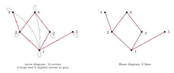
Figure 201: The relation \(x \mid y\) on \({1, \dots, 6}\), as an arrow diagram and as a Hasse diagram. Left: all 14 arrows. The 8 that the steps delete are grey: the 6 loops, and the arrows \(1 \to 4\) and \(1 \to 6\), which the transitive property implies. Right: the 6 that remain, without arrowheads. A number divides another exactly when a path leads from it up to the other, so \(1 \mid 6\) still shows, by way of 2 or 3. 5 is joined only to 1, since it divides none of the others and only 1 divides it.
Reading a Hasse diagram
A Hasse diagram is sufficient to define the relation: nothing was lost in drawing it. To read the relation back, undo the steps:
\(x \mathrel{R} y\) exactly when \(x = y\), or there is a path from \(x\) to \(y\) that goes upward all the way.
- \(x = y\) restores the loops (step 2).
- A path of one line is an arrow that was kept.
- A path of two or more lines restores an implied arrow (step 3).
- “Upward” restores the direction (step 4).
For the six-element example the count comes back as 6 loops, 6 kept arrows and 6 implied arrows, 18 in all.
The same rule reads off the other notions of partial-order-relations:
- Comparable: two different elements are comparable exactly when an upward path joins them, starting from either one.
- Non-comparable: no upward path either way. Two elements drawn at the same height are never comparable, because every line climbs.
- Total order: the whole diagram is a single column, one element above the other.
A path that goes up and then comes down does not count. In the diagram of \(\subseteq\) on \(\mathcal{P}(\{1,2,3\})\) you can get from \(\{1\}\) to \(\{2,3\}\) along lines, but only by going down at some point. \(\{1\} \not\subseteq \{2,3\}\), and the two are not comparable.
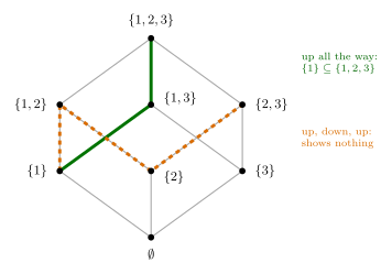
Figure 202: Reading the Hasse diagram of \(\subseteq\) on \(\mathcal{P}({1,2,3})\). The green path climbs at every step, from \({1}\) through \({1,3}\) to \({1,2,3}\), so \({1} \subseteq {1,2,3}\) and the two sets are comparable. The dashed orange path also joins two sets, \({1}\) and \({2,3}\), but it goes up, then down, then up. It does not show a relation. No path from \({1}\) climbs all the way to \({2,3}\), and none climbs from \({2,3}\) to \({1}\), so those two sets are not comparable.
The diagrams in the course so far
| Partial order | Its Hasse diagram | Where |
|---|---|---|
| six elements \(a\) to \(f\) | a column \(a, b, c, d, e\) with \(f\) joined to \(a\) and \(e\) | 2026-09-22-partial-order-relations |
| \(\subseteq\) on \(\mathcal{P}(\{1,2,3\})\) | a cube standing on a corner, 12 lines | 2026-09-22-partial-order-relations |
| divides on \(\{1,\dots,6\}\) | 6 lines, above | above |
| divides on \(\{1,2,4,8,16\}\) | a single column | partial-order-relations |
In the power-set diagram each line adds exactly one element to a set. In the divides diagram above each line multiplies by a prime: \(1 \to 2\), \(1 \to 3\), \(1 \to 5\), \(2 \to 4\), \(2 \to 6\), \(3 \to 6\). In both cases a line is a single smallest step up.
Common mistakes
- Keeping an implied line. If \(x\) is joined up to \(y\) and \(y\) up to \(z\), there is no line from \(x\) to \(z\). A triangle in a Hasse diagram is always wrong.
- A horizontal line. Every line has to climb, or the deleted arrowhead cannot be recovered.
- Putting the larger element lower. The relation reads upward. For divides, 1 is at the bottom. For \(\subseteq\), \(\emptyset\) is.
- Reading only the lines as the relation. The lines are the kept arrows. The relation also contains every loop and every implied arrow.
- Drawing one for a relation that is not a partial order. If two different elements are related both ways, step 1 cannot be done.
- Treating any path as a comparison. The path must go upward at every step.
See also
- partial-order-relations — partial and total orders, and comparable elements
- antisymmetric-relations — the property that lets the arrows all point one way
- relations-on-sets — the full arrow diagram a Hasse diagram is cut down from
- reflexive-symmetric-and-transitive-relations — loops and short cuts, the arrows steps 2 and 3 delete
- 2026-09-22-partial-order-relations — Lecture 25
- practice-problems — §32, with full worked solutions
Incidence Matrices
An incidence matrix writes a graph down by vertices against edges: a row for each vertex, a column for each edge, and in each place the number of times that vertex is incident with that edge. Each column is one edge, so the matrix is in effect the table of endpoints written as numbers. It has a simple shape that makes it easy to check: every column adds to 2, because every edge has two ends, and every row adds to the degree of its vertex. Putting those together proves the Handshake Theorem again. The other matrix of a graph, vertices against vertices, is in adjacency-matrices. Graphs, loops, degree and the Handshake Theorem are in [graphs]. First met in 2026-10-27-matrix-representations-of-graphs.
Definition
The incidence matrix of a graph with vertices \(v_1, v_2, \dots, v_n\) and edges \(e_1, e_2, \dots, e_m\) is the \(n \times m\) matrix \(N = [n_{ij}]\) where each entry \(n_{ij}\) is the number of times vertex \(v_i\) is incident with edge \(e_j\).
Rows are vertices and columns are edges. The entry \(n_{ij}\) is about vertex \(v_i\) and edge \(e_j\), in that order, and the first index is the row. The matrix is \(n \times m\): as many rows as vertices, as many columns as edges. Swapping the roles gives the transpose \(N^{\mathsf T}\), which holds the same information but is not the incidence matrix as this course defines it, so write the vertices down the side and the edges across the top, and label both. Like the adjacency matrix, \(N\) depends on the order chosen for the vertices and for the edges.
An edge has two ends. For a vertex \(v_i\) and an edge \(e_j\) there are three cases:
- \(e_j\) does not have \(v_i\) as an endpoint: \(n_{ij} = 0\).
- \(e_j\) joins \(v_i\) to a different vertex: one end is at \(v_i\), so \(n_{ij} = 1\).
- \(e_j\) is a loop at \(v_i\): both ends are at \(v_i\), so \(n_{ij} = 2\).
So every entry is 0, 1 or 2, and a 2 means a loop.
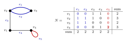
Figure 203: A graph and its incidence matrix, one row for each vertex and one column for each edge. Each column is an edge: e3 has a 1 at each of its endpoints v1 and v2, and the loop e5, in red, has a single 2 at v4, because it meets v4 at both of its ends. The parallel edges e1 and e2, in blue, have the same endpoints and so identical columns. Every column adds to 2, and each row adds to the degree of its vertex: 2, 3, 2, 3.
Columns are edges
The column of \(e_j\) lists how many times each vertex meets \(e_j\). So:
- Every column adds to 2. An edge has exactly two ends, and each end is at one vertex. A column is either two 1s (an edge with two different endpoints, the rows of the 1s) or a single 2 (a loop, at the row of the 2), and 0 everywhere else.
- Parallel edges have identical columns. Two edges with the same endpoints meet every vertex the same number of times. In the figure, \(e_1\) and \(e_2\) are both \((0, 1, 1, 0)\).
- A column is never all zeros, since every edge has at least one endpoint.
Rows are vertices
The row of \(v_i\) lists how many times \(v_i\) meets each edge.
- The row sum is the degree. Adding the row counts the ends of edges at \(v_i\), a loop’s two ends included, which is \(\deg(v_i)\) (graphs). Unlike the adjacency matrix, no correction for loops is needed: the loop’s 2 is already in the row.
- An isolated vertex has a row of zeros. It still gets its row.
The Handshake Theorem again
Add up every entry of \(N\) in two ways.
- Column by column: each of the \(m\) columns adds to 2, so the total is \(2m\).
- Row by row: row \(i\) adds to \(\deg(v_i)\), so the total is \(\deg(v_1) + \cdots + \deg(v_n)\).
The two totals are the same number, so
\[\sum_{i=1}^{n} \deg(v_i) = 2m,\]
which is the Handshake Theorem (graphs). It is the same proof as counting edge ends, with the ends laid out in a table: each entry counts ends of one edge at one vertex. In the figure, the row sums \(2 + 3 + 2 + 3\) and the column sums \(2 + 2 + 2 + 2 + 2\) both come to 10.
Loops
A loop at \(v_i\) is incident with \(v_i\) twice, once at each of its ends, so its column has a 2 in row \(v_i\) and 0 everywhere else. In the figure the loop \(e_5\) is the column \((0, 0, 0, 2)\).
This is what keeps the column sums at 2 and makes the row sums the degrees: the 2 is the loop’s contribution to \(\deg(v_i)\).
The adjacency matrix counts a loop differently. It counts edges, and a loop is one edge, so it puts a 1 on the diagonal (adjacency-matrices). The same loop is a 1 in \(A\) and a 2 in \(N\). A column with a single 1 and nothing else is not a loop. It is not an edge at all, since it has only one end.
Reading a graph off a matrix
Read an incidence matrix one column at a time:
- Draw a dot for each row and label it \(v_1, \dots, v_n\).
- For each column \(e_j\): if it has 1s in rows \(i\) and \(k\), draw an edge \(e_j\) joining \(v_i\) and \(v_k\); if it has a 2 in row \(i\), draw a loop \(e_j\) at \(v_i\).
- Check: every column added to 2, and each vertex’s degree in the drawing is its row sum.
For example,
\[N = \begin{array}{c|ccccc} & e_1 & e_2 & e_3 & e_4 & e_5 \\ \hline v_1 & 1 & 0 & 0 & 2 & 0 \\ v_2 & 1 & 1 & 1 & 0 & 0 \\ v_3 & 0 & 1 & 1 & 0 & 1 \\ v_4 & 0 & 0 & 0 & 0 & 1 \end{array}\]
has every column adding to 2. Column by column: \(e_1\) joins \(v_1\) and \(v_2\); \(e_2\) and \(e_3\) both join \(v_2\) and \(v_3\), identical columns, so they are parallel; \(e_4\) is a loop at \(v_1\); \(e_5\) joins \(v_3\) and \(v_4\).
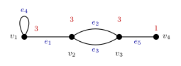
Figure 204: The graph read off the incidence matrix, one column at a time. Columns e2 and e3 are identical, so those two edges are parallel, and column e4 is a single 2 in row v1, so it is a loop at v1. The degrees, in red, are the row sums of the matrix, 3, 3, 3, 1, and they add to 10, twice the 5 edges.
Unlike an adjacency matrix, an incidence matrix names every edge, so the graph comes back with its edge names as well.
Which matrices are incidence matrices
A matrix with at least one row is the incidence matrix of some graph if and only if every entry is a non-negative integer and every column adds to 2. Equivalently, every column is either two 1s and the rest 0, or a single 2 and the rest 0.
The two forms agree: non-negative integers adding to 2 are either \(1 + 1\) or \(2\), with zeros elsewhere.
Proof. (\(\Rightarrow\)) Shown above: each column is an edge, and an edge is two 1s at its two endpoints or a single 2 at the vertex of a loop.
(\(\Leftarrow\)) Let \(M\) be an \(n \times m\) matrix, \(n \ge 1\), whose columns each have one of the two forms. Build a graph with vertices \(v_1, \dots, v_n\) and, for each column \(j\), an edge \(e_j\): if column \(j\) has 1s in rows \(i\) and \(k\), let \(e_j\) join \(v_i\) and \(v_k\); if it has a 2 in row \(i\), let \(e_j\) be a loop at \(v_i\). Then \(v_i\) is incident with \(e_j\) once if \(v_i\) is one of two endpoints, twice if \(e_j\) is a loop at \(v_i\), and not at all otherwise, which is the entry \(m_{ij}\) in every case. So \(M\) is this graph’s incidence matrix. \(\square\)
Only the columns are tested. The rows can be anything, a row of zeros included (an isolated vertex), and the matrix does not have to be square or symmetric. A graph with no edges has no columns at all, and then there is nothing to check.
| Matrix | Column sums | Incidence matrix? |
|---|---|---|
| \(\begin{bmatrix} 1 & 2 \\ 1 & 0 \end{bmatrix}\) | \(2,\ 2\) | yes: an edge \(v_1 v_2\) and a loop at \(v_1\) |
| \(\begin{bmatrix} 1 & 1 \\ 1 & 0 \\ 0 & 0 \end{bmatrix}\) | \(2,\ 1\) | no: the second edge has only one end |
| \(\begin{bmatrix} 1 \\ 1 \\ 1 \end{bmatrix}\) | \(3\) | no: an edge with three ends |
| \(\begin{bmatrix} 0 \\ 2 \\ 0 \end{bmatrix}\) | \(2\) | yes: three vertices, a loop at \(v_2\), and \(v_1\), \(v_3\) isolated |
Four more are worked in 2026-10-27-matrix-representations-of-graphs.
Adjacency and incidence compared
The graph in the figure has both matrices:
\[A = \begin{array}{c|cccc} & v_1 & v_2 & v_3 & v_4 \\ \hline v_1 & 0 & 1 & 0 & 1 \\ v_2 & 1 & 0 & 2 & 0 \\ v_3 & 0 & 2 & 0 & 0 \\ v_4 & 1 & 0 & 0 & 1 \end{array} \qquad\qquad N = \begin{array}{c|ccccc} & e_1 & e_2 & e_3 & e_4 & e_5 \\ \hline v_1 & 0 & 0 & 1 & 1 & 0 \\ v_2 & 1 & 1 & 1 & 0 & 0 \\ v_3 & 1 & 1 & 0 & 0 & 0 \\ v_4 & 0 & 0 & 0 & 1 & 2 \end{array}\]
| Adjacency matrix \(A\) | Incidence matrix \(N\) | |
|---|---|---|
| Size | \(n \times n\) | \(n \times m\) |
| Rows | vertices | vertices |
| Columns | vertices | edges |
| Entry | number of edges with endpoints \(\{v_i, v_j\}\) | number of times \(v_i\) is incident with \(e_j\) |
| Entries can be | any non-negative integer | 0, 1 or 2 |
| A loop at \(v_i\) | 1 on the diagonal, at \(a_{ii}\) | 2 in its column, at row \(v_i\) |
| Parallel edges | one entry bigger than 1 | identical columns |
| Shape | square and symmetric | any; each column adds to 2 |
| \(\deg(v_i)\) | row sum plus \(a_{ii}\) | row sum |
| Number of edges | sum on and above the diagonal | number of columns |
| Edge names | not recorded | one column per named edge |
From \(N\) to \(A\). Off the diagonal, \(a_{ij}\) is the number of columns with a 1 in both row \(i\) and row \(j\). On the diagonal, \(a_{ii}\) is the number of columns with a 2 in row \(i\). In \(N\) above, two columns (\(e_1\) and \(e_2\)) have 1s in rows \(v_2\) and \(v_3\), so \(a_{23} = 2\), and one column (\(e_5\)) has a 2 in row \(v_4\), so \(a_{44} = 1\).
From \(A\) to \(N\), the edges first have to be named, since \(A\) only says how many edges join each pair. Any naming gives an incidence matrix of the same graph, with its columns in a different order.
\(A\) is the more compact when there are many edges. \(N\) is the one to use when the edges themselves matter, as in listing an Euler circuit edge by edge, which is done from an incidence matrix in 2026-10-27-matrix-representations-of-graphs.
Common mistakes
- Swapping rows and columns. In this course the vertices are the rows and the edges are the columns. The transpose has the same information but is not the incidence matrix as defined here.
- Writing 1 for a loop. A loop meets its vertex twice, so it is a 2. A column with a single 1 has only one end and is not an edge.
- Adding a loop correction to the row sum. That is for the adjacency matrix. In \(N\) the row sum already is the degree.
- Checking the rows, or symmetry, instead of the columns. Whether a matrix is an incidence matrix is decided by its columns alone: each must add to 2.
- Leaving out an isolated vertex. Every vertex has a row, even if it is all zeros.
- Leaving off the labels. The matrix depends on the order of the vertices and of the edges.
See also
- adjacency-matrices — the vertex-by-vertex matrix, where a loop counts 1
- [graphs] — loops, parallel edges, degree and the Handshake Theorem
- euler-circuits-and-trails — the even-degree test for an Euler circuit
- 2026-10-27-matrix-representations-of-graphs — Lecture 35
- practice-problems — §45, with full worked solutions
Inclusion/Exclusion
How to count a union of finite sets that overlap. The addition rule adds the sizes of sets only when they are disjoint; when an element can be in more than one set, adding the sizes counts it more than once. Inclusion/exclusion corrects this by subtracting the sizes of the pairwise intersections, adding back the triple intersections, and so on with alternating signs. This note covers the rule for two and three sets, why it counts every element exactly once, a proof of the three-set rule from the two-set rule, the general rule for \(n\) sets, counting “none of them” through the complement, counting multiples with the floor function, and the same rule for probabilities. The addition and difference rules it extends are in counting-principles. First met in 2026-10-20-inclusion-exclusion.
Two sets
Inclusion/exclusion for two sets. For finite sets \(A\) and \(B\), \[|A \cup B| = |A| + |B| - |A \cap B|.\]
Why. Split \(A \cup B\) into three disjoint pieces: \(A - B\), \(A \cap B\) and \(B - A\). Then \(|A|\) counts the first two pieces and \(|B|\) counts the last two, so \(|A| + |B|\) counts \(A \cap B\) twice and the other two pieces once each. Subtracting \(|A \cap B|\) once leaves every element of the union counted once.
| \(A - B\) | \(A \cap B\) | \(B - A\) | |
|---|---|---|---|
| counted by \(\vert A\vert\) | 1 | 1 | 0 |
| counted by \(\vert B\vert\) | 0 | 1 | 1 |
| removed by \(-\vert A \cap B\vert\) | 0 | \(-1\) | 0 |
| total | 1 | 1 | 1 |
If \(A \cap B = \emptyset\), the correction is 0 and the rule is the addition rule, \(|A \cup B| = |A| + |B|\) (counting-principles). The three-piece split is also the quickest check on any two-set answer: once \(|A \cap B|\) is known, \(|A - B| = |A| - |A \cap B|\) and \(|B - A| = |B| - |A \cap B|\), and the pieces together with the outside must add to the size of the universe.
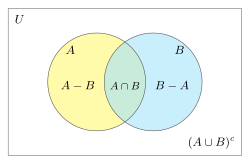
Figure 205: A universe \(U\) split by two sets into four disjoint regions. The circle \(A\) is the regions \(A - B\) and \(A \cap B\), and the circle \(B\) is \(A \cap B\) and \(B - A\), so the overlap is the one region inside both circles and is counted by both \(|A|\) and \(|B|\). Everything outside both circles is the complement \((A \cup B)^c\), the elements in neither set.
Three sets
Inclusion/exclusion for three sets. For finite sets \(A\), \(B\) and \(C\), \[|A \cup B \cup C| = |A| + |B| + |C| - |A \cap B| - |A \cap C| - |B \cap C| + |A \cap B \cap C|.\]
Three groups of terms, with alternating signs: the three single sets added, the three pairwise intersections subtracted, the one triple intersection added.
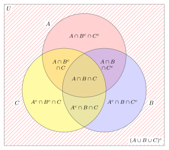
Figure 206: The eight disjoint regions into which three sets cut a universe \(U\), each named by which of \(A\), \(B\) and \(C\) it lies inside and which outside. Every term of the formula is a union of some of these regions: \(|A|\) covers the four regions inside \(A\), \(|A \cap B|\) the two inside both \(A\) and \(B\), and \(|A \cap B \cap C|\) the centre alone. The hatched region outside all three circles is \((A \cup B \cup C)^c = A^c \cap B^c \cap C^c\), the elements in none of the sets.
Every region counted once
Three overlapping circles make seven regions inside the union. Each region is described by how many of the three sets it lies in, and that number decides how the formula counts it.
- In exactly one set, say \(A\) only. Counted once by \(|A|\), and in none of the intersections. Net: 1.
- In exactly two sets, say \(A\) and \(B\) but not \(C\). Counted by \(|A|\) and \(|B|\), so twice, and removed once, by \(|A \cap B|\). It is not in \(A \cap C\) or \(B \cap C\), because those need \(C\). Net: \(2 - 1 = 1\).
- In all three. Counted three times by the singles, removed three times by the pairs, since it is in \(A \cap B\), \(A \cap C\) and \(B \cap C\), and added once by the triple. Net: \(3 - 3 + 1 = 1\).
This is why the triple intersection is added back once. After the pairs are subtracted, the centre has been counted \(3 - 3 = 0\) times, one short of the 1 it needs. Adding \(|A \cap B \cap C|\) twice would leave it counted twice.
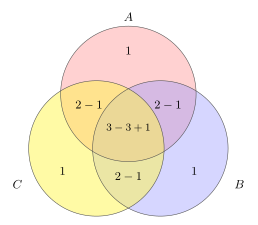
Figure 207: Each region of a three-set Venn diagram labelled with how the formula counts it: the number of single sets containing it, minus the number of pairwise intersections containing it, plus the triple intersection if it is in all three. A region in one set is counted \(1\); a region in two sets \(2 - 1\); the centre \(3 - 3 + 1\). Every region comes to exactly 1.
Proving the three-set rule from the two-set rule
The three-set rule is three applications of the two-set rule, \(|X \cup Y| = |X| + |Y| - |X \cap Y|\), together with the set identities (formula-sheet).
\[\begin{aligned} |A \cup B \cup C| &= |A \cup (B \cup C)| && \text{associative law (2a)} \\ &= |A| + |B \cup C| - |A \cap (B \cup C)| && X = A,\ Y = B \cup C \\ &= |A| + |B| + |C| - |B \cap C| - |A \cap (B \cup C)| && X = B,\ Y = C \\ &= |A| + |B| + |C| - |B \cap C| - |(A \cap B) \cup (A \cap C)| && \text{distributive law (3b)} \\ &= |A| + |B| + |C| - |B \cap C| - \big(|A \cap B| + |A \cap C| - |A \cap B \cap C|\big) && X = A \cap B,\ Y = A \cap C \\ &= |A| + |B| + |C| - |A \cap B| - |A \cap C| - |B \cap C| + |A \cap B \cap C|. && \end{aligned}\]
The fifth line uses \((A \cap B) \cap (A \cap C) = A \cap B \cap C\), which is the commutative and associative laws (1b, 2b) to bring the two \(A\)’s together and the idempotent law (7b), \(A \cap A = A\). The triple term is subtracted inside a bracket that is itself subtracted, which is where its \(+\) sign comes from. Each step is drawn in 2026-10-20-inclusion-exclusion.
The same move, splitting off the last set and applying the two-set rule, proves the rule for four sets from the rule for three, and so on: it is an induction on \(n\) (mathematical-induction).
The general rule
Inclusion/exclusion for \(n\) sets. For finite sets \(A_1, A_2, \dots, A_n\), \[|A_1 \cup \cdots \cup A_n| = \sum_{1 \leq i \leq n} |A_i| - \sum_{1 \leq i < j \leq n} |A_i \cap A_j| + \sum_{1 \leq i < j < k \leq n} |A_i \cap A_j \cap A_k| - \cdots + (-1)^{n+1} |A_1 \cap \cdots \cap A_n|.\]
Add the singles, subtract the pairs, add the triples, subtract the four-way intersections, and keep alternating up to the intersection of all \(n\), whose sign is \(+\) when \(n\) is odd and \(-\) when \(n\) is even. There are \(\binom{n}{k}\) intersections of \(k\) sets, so the formula has \(2^n - 1\) terms in all: 3 for two sets, 7 for three, 15 for four.
Written as a single sum over the non-empty sets \(S\) of indices, with \(\bigcap_{t \in S} A_t\) the intersection of the \(A_t\) for \(t \in S\) (for \(S = \{2, 3, 6\}\), that is \(A_2 \cap A_3 \cap A_6\)):
\[|A_1 \cup A_2 \cup \cdots \cup A_n| = \sum_{\emptyset \neq S \subseteq \{1, \dots, n\}} (-1)^{|S|+1} \left| \bigcap_{t \in S} A_t \right|.\]
Why each element is counted once. Take an element \(x\) of the union, and say it lies in exactly \(m \geq 1\) of the sets. A term \(|\bigcap_{t \in S} A_t|\) counts \(x\) exactly when every set in \(S\) contains \(x\), that is, when \(S\) is a non-empty subset of the \(m\) indices of sets containing \(x\). There are \(\binom{m}{k}\) such \(S\) of size \(k\), so \(x\) is counted
\[\binom{m}{1} - \binom{m}{2} + \binom{m}{3} - \cdots + (-1)^{m+1}\binom{m}{m} = 1 - (1 - 1)^m = 1\]
times. The middle step is the binomial theorem applied to \((1 - 1)^m = \sum_{k=0}^{m} \binom{m}{k}(-1)^k\), which is 0 because \(m \geq 1\) (binomial-coefficients). For \(m = 1, 2, 3, 4\) the counts are \(1\), \(2 - 1\), \(3 - 3 + 1\) and \(4 - 6 + 4 - 1\).
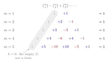
Figure 208: How the general formula counts an element lying in exactly \(m\) of the sets, for \(m = 1\) to \(5\). Row \(m\) lists \(\binom{m}{k}\), the number of intersections of \(k\) of those \(m\) sets, each carrying the sign of its group: \(+\) for odd \(k\) and \(-\) for even \(k\). The grey entry is \(\binom{m}{0} = 1\), which would belong to the empty set of indices and is not a term. Flipping the sign of every coloured entry and adding the grey 1 gives the expansion of \((1 - 1)^m = 0\), so the coloured entries themselves sum to \(1 - (1 - 1)^m = 1\) in every row.
None of them: the complement
Inclusion/exclusion counts the elements in at least one of the sets. The elements in none of them are everything else, so inside a universe \(U\),
\[|(A \cup B)^c| = |U| - |A \cup B| = |U| - |A| - |B| + |A \cap B|,\]
\[|(A \cup B \cup C)^c| = |U| - |A| - |B| - |C| + |A \cap B| + |A \cap C| + |B \cap C| - |A \cap B \cap C|.\]
This is the difference rule (counting-principles) applied to the union. By De Morgan’s law (9a), \((A \cup B)^c = A^c \cap B^c\): “in neither \(A\) nor \(B\)” and “outside the union” are the same set. Questions phrased as “neither … nor”, “none of”, or “not divisible by any of” are complements of a union.
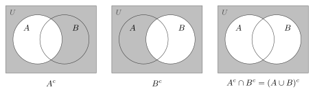
Figure 209: The elements in neither \(A\) nor \(B\). The part of \(U\) outside \(A\) and the part outside \(B\) overlap in exactly the region outside both circles, which is the complement of the union: \(A^c \cap B^c = (A \cup B)^c\). Counting that region is \(|U| - |A \cup B|\), and inclusion/exclusion supplies \(|A \cup B|\).
Running it backwards. The two-set rule links four numbers, \(|A|\), \(|B|\), \(|A \cap B|\) and \(|A \cup B|\), and any three determine the fourth. A question that gives the sizes of \(A\), \(B\) and the “neither” region, and asks for “both”, finds the union from the complement first and then solves for the intersection:
\[|A \cap B| = |A| + |B| - |A \cup B| = |A| + |B| - \big(|U| - |(A \cup B)^c|\big).\]
Counting multiples
The commonest use of inclusion/exclusion is counting integers with divisibility conditions. Two facts do all the work.
- The multiples of \(d\) in \(\{1, 2, \dots, N\}\) are \(d, 2d, \dots, kd\) for the largest \(k\) with \(kd \leq N\), that is, \(k \leq N/d\). So there are \(\lfloor N/d \rfloor\) of them. When \(d\) divides \(N\) the floor is not needed: \(105/3 = 35\).
- Being divisible by both \(a\) and \(b\) is being divisible by \(\operatorname{lcm}(a, b)\) (gcd-lcm-and-euclidean-algorithm). When \(a\) and \(b\) have no common factor, \(\operatorname{lcm}(a, b) = ab\), so the multiples of both 3 and 5 are the multiples of 15. When they share a factor it is smaller than \(ab\): the multiples of both 4 and 6 are the multiples of 12, not of 24.
The method, for “how many of \(1, \dots, N\) are divisible by none of \(a\), \(b\), \(c\)”:
- Let \(A\), \(B\), \(C\) be the multiples of \(a\), \(b\), \(c\) in \(\{1, \dots, N\}\).
- Count each with \(\lfloor N/d \rfloor\), using the lcm for each intersection.
- Combine with inclusion/exclusion to get \(|A \cup B \cup C|\).
- Subtract from \(N\).
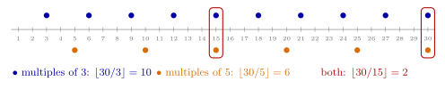
Figure 210: The integers 1 to 30, with the multiples of 3 marked above the line and the multiples of 5 below. There are \(\lfloor 30/3 \rfloor = 10\) multiples of 3 and \(\lfloor 30/5 \rfloor = 6\) of 5, but 15 and 30, the multiples of \(\operatorname{lcm}(3, 5) = 15\), are marked twice. So \(10 + 6 - 2 = 14\) integers are divisible by 3 or 5, and the other 16 by neither.
With probabilities
When all outcomes in a finite sample space \(S\) are equally likely, \(P(E) = |E|/|S|\) (probability). Dividing the two-set rule through by \(|S|\) gives
\[P(A \cup B) = P(A) + P(B) - P(A \cap B),\]
and the three-set and \(n\)-set rules divide through in the same way. The probability that neither happens is \(1 - P(A \cup B)\). Either count first and divide at the end, or divide first and combine probabilities; the answer is the same.
Worked: divisible by 2, 3 or 5
How many of the integers \(1, 2, \dots, 1000\) are divisible by none of 2, 3 and 5?
Let \(A\), \(B\), \(C\) be the multiples of 2, 3 and 5 in \(\{1, \dots, 1000\}\). The numbers are pairwise coprime, so each intersection is the multiples of the product. Not every division is exact this time.
\[|A| = \left\lfloor \tfrac{1000}{2} \right\rfloor = 500, \quad |B| = \left\lfloor \tfrac{1000}{3} \right\rfloor = 333, \quad |C| = \left\lfloor \tfrac{1000}{5} \right\rfloor = 200,\]
\[|A \cap B| = \left\lfloor \tfrac{1000}{6} \right\rfloor = 166, \quad |A \cap C| = \left\lfloor \tfrac{1000}{10} \right\rfloor = 100, \quad |B \cap C| = \left\lfloor \tfrac{1000}{15} \right\rfloor = 66, \quad |A \cap B \cap C| = \left\lfloor \tfrac{1000}{30} \right\rfloor = 33.\]
\[|A \cup B \cup C| = 500 + 333 + 200 - 166 - 100 - 66 + 33 = 734,\]
so \(1000 - 734 = 266\) are divisible by none of 2, 3 and 5. A direct count over \(1, \dots, 1000\) agrees.
Worked: the lcm, not the product
How many of the integers \(1, 2, \dots, 100\) are divisible by 4 or by 6?
Let \(A\) be the multiples of 4 and \(B\) the multiples of 6. Then \(|A| = \lfloor 100/4 \rfloor = 25\) and \(|B| = \lfloor 100/6 \rfloor = 16\). A number divisible by both 4 and 6 is divisible by \(\operatorname{lcm}(4, 6) = 12\), so \(|A \cap B| = \lfloor 100/12 \rfloor = 8\). Hence
\[|A \cup B| = 25 + 16 - 8 = 33.\]
Using \(4 \cdot 6 = 24\) for the intersection gives \(\lfloor 100/24 \rfloor = 4\) and the wrong answer 37. The number 12 is divisible by both 4 and 6 but not by 24.
Worked: both, from neither
In a class of 60 students, 35 study French, 28 study German and 10 study neither. How many study both?
Let \(F\) and \(G\) be the students studying French and German. The students studying at least one are everyone except the 10, so \(|F \cup G| = 60 - 10 = 50\). Then
\[|F \cap G| = |F| + |G| - |F \cup G| = 35 + 28 - 50 = 13.\]
Check: \(35 - 13 = 22\) French only, \(28 - 13 = 15\) German only, 13 both and 10 neither, and \(22 + 15 + 13 + 10 = 60\).
Worked: at least one six
Two fair dice are rolled. What is the probability that at least one shows a six?
The 36 ordered pairs of results are equally likely. Let \(A\) be “the first die shows 6” and \(B\) “the second die shows 6”. Each has 6 outcomes, and \(A \cap B\) is the single outcome \((6, 6)\). So
\[P(A \cup B) = P(A) + P(B) - P(A \cap B) = \frac{6}{36} + \frac{6}{36} - \frac{1}{36} = \frac{11}{36}.\]
The answer \(\frac{12}{36} = \frac13\), from adding without the correction, counts the double six twice. The complement agrees: no six on either die has \(5 \cdot 5 = 25\) outcomes, and \(1 - \frac{25}{36} = \frac{11}{36}\).
Common mistakes
- Adding overlapping sets. \(|A| + |B|\) is \(|A \cup B|\) only when \(A\) and \(B\) are disjoint. Otherwise it counts every element of \(A \cap B\) twice.
- The wrong sign on the triple term. \(|A \cap B \cap C|\) is added. Subtracting it, as if every intersection were subtracted, leaves the centre counted \(3 - 3 - 1 = -1\) times.
- Leaving out the triple term. Subtracting the three pairs and stopping counts the centre 0 times.
- “Neither” as \(|U| - |A| - |B|\). That removes \(A \cap B\) twice. The elements in neither are \(|U| - |A \cup B| = |U| - |A| - |B| + |A \cap B|\).
- The product instead of the lcm. Divisible by 4 and 6 is divisible by 12, not 24. The product is right only when the numbers share no factor.
- Forgetting the floor. There are \(\lfloor 1000/3 \rfloor = 333\) multiples of 3 up to 1000, not \(333.\overline{3}\).
- Including the empty set of indices. In the sum over index sets \(S\), \(S\) ranges over the non-empty subsets of \(\{1, \dots, n\}\). There is no intersection of no sets among the terms.
- Reading the “neither” group wrongly. “Came to class and scored below 60%” is outside both “did not come” and “scored at least 60%”: it is \((A \cup B)^c\), not \(A \cap B\) or \(A^c\) alone.
See also
- 2026-10-20-inclusion-exclusion — Lecture 32, with every question worked in full
- counting-principles — the addition rule for disjoint sets and the difference rule
- sets-and-set-notation — unions, intersections and complements
- formula-sheet — the numbered set identities used in the proof
- gcd-lcm-and-euclidean-algorithm — the lcm, for intersections of sets of multiples
- binomial-coefficients — \(\binom{m}{k}\) and the binomial theorem behind the general rule
- [probability] — probability by counting equally likely outcomes
- practice-problems — §41, with full worked solutions
The Integers Modulo n
\(\mathbb{Z}_n\) is the set of equivalence classes of congruence mod \(n\). It is a number system with exactly \(n\) elements, in which addition and multiplication are done on classes. Congruence itself is in modular-arithmetic, and equivalence classes in equivalence-classes-and-partitions. Under addition \(\mathbb{Z}_n\) is one of the course’s standard [groups], and when \(n\) is prime it is a field, with division by every non-zero class ([fields]). First met in 2026-09-24-definitions-and-examples-of-groups.
The set \(\mathbb{Z}_n\)
Fix \(n \in \mathbb{Z}^{+}\). Congruence mod \(n\) is an equivalence relation on \(\mathbb{Z}\), \[m \mathrel{R} k \iff m \equiv k \pmod n \iff n \mid (m - k),\] and its classes partition \(\mathbb{Z}\). \(\mathbb{Z}_n\) is the set of those classes: \[\mathbb{Z}_n = \{[0], [1], [2], \dots, [n-1]\}.\]
For \(n = 10\): \[\mathbb{Z}_{10} = \{[0], [1], [2], [3], [4], [5], [6], [7], [8], [9]\}\] \[[0] = \{\dots, -30, -20, -10, 0, 10, 20, 30, \dots\}, \qquad [1] = \{\dots, -29, -19, -9, 1, 11, 21, 31, \dots\}\]
- \(\mathbb{Z}_n\) has exactly \(n\) elements. Every integer leaves exactly one of the remainders \(0, 1, \dots, n-1\) on division by \(n\) (modular-arithmetic), so every integer is in exactly one of the \(n\) classes.
- Each element is an infinite set of integers. \([1]\) is not the number 1. It is the set of all integers congruent to 1.
- Each class has many names. \([0] = [10] = [30]\) and \([1] = [21] = [-9]\). In general \([a] = [b]\) exactly when \(a \equiv b \pmod n\) (equivalence-classes-and-partitions).
We usually use \([0], [1], \dots, [n-1]\) as representatives for the equivalence classes of \(\mathbb{Z}_n\).
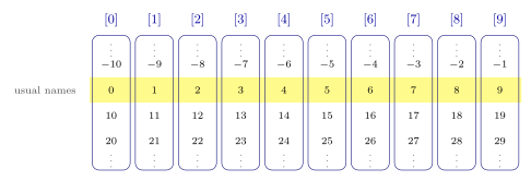
Figure 211: The integers from \(-10\) to 29 written in rows of ten. Each column is one element of \(\mathbb{Z}_{10}\): going down a column adds 10, so everything in a column is congruent mod 10. The whole of \(\mathbb{Z}\) is sorted into these ten columns, and \(\mathbb{Z}_{10}\) is the set of the ten columns. The shaded row holds the usual representatives, 0 to 9. Any other number in a column names the same class, so \([21] = [1]\) and \([-1] = [9]\).
Adding and multiplying classes
Define binary operations \(+\) (plus/addition) and \(\cdot\) (times/multiplication) on \(\mathbb{Z}_n\) as follows. For all \([a], [b] \in \mathbb{Z}_n\), \[[a] + [b] = [a + b] \qquad\text{and}\qquad [a] \cdot [b] = [ab].\]
To combine two classes, combine a representative of each in the ordinary way and take the class of the result. In \(\mathbb{Z}_{10}\): \([8] + [9] = [17] = [7]\) and \([8] \cdot [9] = [72] = [2]\).
Any representative can be used
when doing arithmetic in \(\mathbb{Z}_n\), any representative of the equivalence classes can be used.
The definition \([a] + [b] = [a + b]\) computes with the particular names \(a\) and \(b\), and each class has infinitely many names. The boxed sentence says the result does not depend on which names are used.
The reason is the lemma of modular-arithmetic: if \(a \equiv a' \pmod n\) and \(b \equiv b' \pmod n\), then \[a + b \equiv a' + b' \pmod n \qquad\text{and}\qquad ab \equiv a'b' \pmod n.\] In the language of classes, if \([a] = [a']\) and \([b] = [b']\) then \([a + b] = [a' + b']\) and \([ab] = [a'b']\).
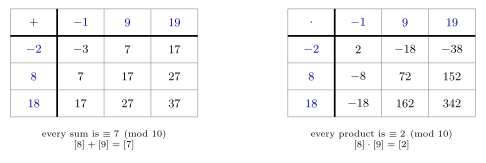
Figure 212: \([8] + [9]\) and \([8] \cdot [9]\) in \(\mathbb{Z}_{10}\), computed with three different representatives of each class: \(-2\), 8 and 18 for \([8]\) down the side, and \(-1\), 9 and 19 for \([9]\) across the top. The sums are not all the same integer, but every one of them is congruent to 7. The products are not all the same integer, but every one is congruent to 2. Whichever representatives are used, \([8] + [9] = [7]\) and \([8] \cdot [9] = [2]\).
Choosing a convenient representative
Since any representative will do, pick the one that makes the arithmetic easy, and reduce at any stage. For example:
\[\begin{aligned} ([8] + [9]) \cdot ([6] + [7]) &= ([8] + [-1]) \cdot ([6] + [-3]) \\ &= [7] \cdot [3] = [21] = [1]. \end{aligned}\]
\([9]\) became \([-1]\) and \([7]\) became \([-3]\). A representative just below a multiple of \(n\) is often better written as a small negative number. Without the swap the same calculation is \([17] \cdot [13] = [221] = [1]\).
\((\mathbb{Z}_n, +)\) is a group
For every \(n \in \mathbb{Z}^{+}\), \((\mathbb{Z}_n, +)\) is a group. The check of the four properties (groups):
- Closure. \([a] + [b] = [a + b]\), which is a class in \(\mathbb{Z}_n\).
- Associativity. \(([a] + [b]) + [c] = [(a + b) + c] = [a + (b + c)] = [a] + ([b] + [c])\). It is inherited from addition of integers.
- Identity. \([0]\), since \([0] + [a] = [a] + [0] = [a]\).
- Inverses. \([a]^{-1} = [-a]\), since \([a] + [-a] = [-a] + [a] = [0]\). With the usual names, \([-a] = [n - a]\).
It is abelian, because \([a] + [b] = [a + b] = [b + a] = [b] + [a]\).
For \(n = 3\), one of the eight candidates of groups:
| \(+\) | \([0]\) | \([1]\) | \([2]\) |
|---|---|---|---|
| \(\mathbf{[0]}\) | \([0]\) | \([1]\) | \([2]\) |
| \(\mathbf{[1]}\) | \([1]\) | \([2]\) | \([0]\) |
| \(\mathbf{[2]}\) | \([2]\) | \([0]\) | \([1]\) |
Here the group inverse of \([1]\) is \([2]\), because \([1] + [2] = [0]\). In an additive group the “inverse” is the negative.
Multiplication: \(\mathbb{Z}_n - \{[0]\}\)
Multiplication of classes is closed, associative and commutative on \(\mathbb{Z}_n\), with identity \([1]\). But \((\mathbb{Z}_n, \cdot)\) is not a group when \(n > 1\): \([0] \cdot [a] = [0]\) for every \([a]\), so \([0]\) has no inverse. This is the same obstacle as 0 in \((\mathbb{R}, \cdot)\), and the same repair is tried, removing it.
| Group under multiplication? | Worked in | |
|---|---|---|
| \(\mathbb{Z}_5 - \{[0]\}\) | yes | 2026-09-24-definitions-and-examples-of-groups; table in practice-problems, Q4 |
| \(\mathbb{Z}_7 - \{[0]\}\) | yes | 2026-09-24-definitions-and-examples-of-groups |
| \(\mathbb{Z}_9 - \{[0]\}\) | no: not closed, \([3] \cdot [3] = [9] = [0]\) | the same practice set, Q1 |
| \(\{[1],[2],[4],[5],[7],[8]\}\) in \(\mathbb{Z}_9\) | yes | the same practice set, Q3 |
| \(\mathbb{Z}_4 - \{[0]\}\) | no: not closed, \([2] \cdot [2] = [4] = [0]\) | 2026-10-08-definitions-and-examples-of-fields |
| \(\mathbb{Z}_{15} - \{[0]\}\) | no: not closed, \([3] \cdot [5] = [15] = [0]\) | 2026-10-08-definitions-and-examples-of-fields |
For \(n = 9\), removing \([0]\) is not enough. \([3]\) and \([6]\) multiply into \([0]\), and removing those as well leaves a group.
The rule: \(\mathbb{Z}_n - \{[0]\}\) is a group under multiplication exactly when \(n\) is prime. When \(n = rs\) is composite, with \(1 < r, s < n\), the non-zero classes \([r]\) and \([s]\) have \([r] \cdot [s] = [n] = [0]\), and closure fails, as for \(9 = 3 \cdot 3\), \(4 = 2 \cdot 2\) and \(15 = 3 \cdot 5\). When \(n\) is prime, no product of non-zero classes is \([0]\) and every non-zero class has an inverse. Why is in fields.
\(\mathbb{Z}_p\) is a field
\((\mathbb{Z}_p, +, \cdot)\) is a field when \(p\) is prime. All three conditions of fields hold:
- \((\mathbb{Z}_p, +)\) is an abelian group, as above.
- \((\mathbb{Z}_p - \{[0]\}, \cdot)\) is an abelian group, by the rule just stated.
- The distributive laws are inherited from the integers: \([a] \cdot ([b] + [c]) = [a(b + c)] = [ab + ac] = [a][b] + [a][c]\).
So in \(\mathbb{Z}_p\) every class can be subtracted and every non-zero class divided by, and every equation \([a]x + [b] = [c]\) with \([a] \neq [0]\) has exactly one solution (fields). For composite \(n\), \(\mathbb{Z}_n\) is not a field. \(\mathbb{Z}_7\) is, and \(\mathbb{Z}_4\) and \(\mathbb{Z}_{15}\) are not (2026-10-08-definitions-and-examples-of-fields).
Finding a multiplicative inverse
The inverse of \([a]\) is the class \([b]\) with \(ab \equiv 1 \pmod n\). Read it from the Cayley table, as in 2026-09-24-definitions-and-examples-of-groups, or search: in \(\mathbb{Z}_7\), \([3] \cdot [5] = [15] = [1]\), so \([3]^{-1} = [5]\). This is the relation \(xy \equiv 1 \pmod 7\), whose arrow diagram is in 2026-09-17-relations-reflexivity-symmetry-transitivity: each non-zero number is joined to its inverse.
When there is no table, there are three ways in:
- List the multiples. Write \(a, 2a, 3a, \dots\) mod \(p\), each one the previous plus \(a\), reduced, until \(1\) appears. For \([10]\) in \(\mathbb{Z}_{17}\) the list is \(10, 3, 13, 6, 16, 9, 2, 12, 5, 15, 8, 1\), so \(10 \cdot 12 \equiv 1\) and \([10]^{-1} = [12]\). The search is drawn in 2026-10-08-definitions-and-examples-of-fields. In \(\mathbb{Z}_p\) it always succeeds within \(p - 1\) steps, because the multiples of a non-zero class run through every non-zero class.
- Stop at \(-1\). If \(ab \equiv -1\), then \(a \cdot (-b) \equiv 1\), so \([a]^{-1} = [-b]\). In the same list, \(10 \cdot 5 = 50 \equiv 16 = -1 \pmod{17}\), so \([10]^{-1} = [-5] = [12]\) after five steps instead of twelve.
- Quick cases. \([1]^{-1} = [1]\) and \([p - 1]^{-1} = [p - 1]\), since \((-1)(-1) = 1\). For odd \(p\), \([2]^{-1} = [\frac{p+1}{2}]\), since \(2 \cdot \frac{p+1}{2} = p + 1 \equiv 1\). In \(\mathbb{Z}_{11}\) that gives \([2]^{-1} = [6]\).
The inverses in three small fields, each pair being inverses of each other:
| \(p\) | Own inverse | Pairs |
|---|---|---|
| 5 | \([1]\), \([4]\) | \([2] \leftrightarrow [3]\) |
| 7 | \([1]\), \([6]\) | \([2] \leftrightarrow [4]\), \(\ [3] \leftrightarrow [5]\) |
| 11 | \([1]\), \([10]\) | \([2] \leftrightarrow [6]\), \(\ [3] \leftrightarrow [4]\), \(\ [5] \leftrightarrow [9]\), \(\ [7] \leftrightarrow [8]\) |
In a composite \(\mathbb{Z}_n\) the search can fail. The multiples of \([2]\) in \(\mathbb{Z}_6\) are \([2], [4], [0], [2], \dots\), and \([1]\) never appears, so \([2]\) has no inverse there.
Notation
- Three ways to say one thing. \(n \mid (a - b)\), \(\ a \equiv b \pmod n\), and \([a] = [b]\) in \(\mathbb{Z}_n\) are the same statement. The first is about divisibility, the second about integers, the third about classes.
- \(=\) for classes, \(\equiv\) for integers. \([7] = [0]\) in \(\mathbb{Z}_7\) is true. \(7 = 0\) is false. \(7 \equiv 0 \pmod 7\) is true.
- Brackets are often dropped. The practice problems write \(\mathbb{Z}_9 - \{0\} = \{1, 2, \dots, 8\}\) and “\(2 \cdot 5 = 10 \equiv 1 \pmod 9\)” for what is written here as \(\mathbb{Z}_9 - \{[0]\}\) and \([2] \cdot [5] = [10] = [1]\). It is the same arithmetic.
- The \(-\) in \(\mathbb{Z}_7 - \{[0]\}\) is set difference (sets-and-set-notation): the set \(\mathbb{Z}_7\) with the one element \([0]\) removed.
- \(\bmod\) again. The remainder \(a \bmod n\) is the usual representative of \([a]\) (modular-arithmetic).
Common mistakes
- Treating \([a]\) as the integer \(a\). \([9] = [-1]\) in \(\mathbb{Z}_{10}\), but \(9 \neq -1\).
- Thinking \(\mathbb{Z}_n\) is infinite. It has \(n\) elements. Each element is an infinite set.
- Using the wrong inverse. In \((\mathbb{Z}_7, +)\) the inverse of \([3]\) is \([4]\). In \((\mathbb{Z}_7 - \{[0]\}, \cdot)\) it is \([5]\). Look at the operation first.
- Dividing. There is no \([\frac12]\). An “inverse of \([2]\)” under multiplication means a class \([b]\) with \([2][b] = [1]\), and it may not exist. In \(\mathbb{Z}_p\) it always does: in \(\mathbb{Z}_{11}\) it is \([6]\), so “dividing by 2” there means multiplying by \([6]\).
- Mixing up the two inverses. To undo \(+ [3]\) in \(\mathbb{Z}_{11}\), add \(-[3] = [8]\). To undo \([2] \cdot\), multiply by \([2]^{-1} = [6]\).
- Not checking closure after removing elements. \(\mathbb{Z}_9 - \{[0]\}\) is the example.
See also
- modular-arithmetic — congruence, remainders, and the lemma that makes class arithmetic work
- equivalence-classes-and-partitions — classes and representatives in general
- [groups] — the definition \(\mathbb{Z}_n\) is checked against
- [fields] — why \(\mathbb{Z}_n\) is a field exactly when \(n\) is prime, and solving equations in \(\mathbb{Z}_p\)
- subgroups-and-cyclic-groups — cyclic subgroups and cyclic groups; \((\mathbb{Z}_n, +)\) is cyclic, generated by \([1]\)
- cayley-tables — the tables for \(\mathbb{Z}_7 - \{[0]\}\) and \(\mathbb{Z}_5 - \{[0]\}\) and how to read them
- 2026-09-24-definitions-and-examples-of-groups — Lecture 26 · 2026-09-21-equivalence-relations — Lecture 24, where the classes of congruence mod 3 are drawn
- 2026-10-06-elementary-properties-of-groups — Lecture 27, where powers and cyclic subgroups are worked in \(\mathbb{Z}_7 - \{[0]\}\), \(\mathbb{Z}_{11} - \{[0]\}\) and \(\mathbb{Z}_8\)
- 2026-10-08-definitions-and-examples-of-fields — Lecture 28, where \(\mathbb{Z}_4\), \(\mathbb{Z}_7\) and \(\mathbb{Z}_{15}\) are tested and equations are solved in \(\mathbb{Z}_{11}\) and \(\mathbb{Z}_{17}\)
- practice-problems — §33, with full worked solutions
- practice-problems — §36, equations in \(\mathbb{Z}_5\), \(\mathbb{Z}_{11}\), \(\mathbb{Z}_{13}\) and \(\mathbb{Z}_{19}\)
Inverse Functions
When a function can be run backwards, what the backwards function is, and the one notational trap: \(f^{-1}\) means two different things, and the braces tell you which. Builds on one-to-one-and-onto-functions; the preimage half is from functions-on-general-sets; the lecture is 2026-09-07-functions-one-to-one-onto-inverse.
Bijections have inverses
A function that is both one-to-one and onto is said to be a bijection.
A bijection \(f : X \to Y\) has an inverse function \(f^{-1} : Y \to X\), where for all \(y \in Y\), \[f^{-1}(y) = x \text{ where } x \text{ is the unique } x \in X \text{ such that } f(x) = y.\]
Note the direction: \(f : X \to Y\) gives \(f^{-1} : Y \to X\). The inverse’s domain is \(f\)’s co-domain and vice versa.
The definition is exactly one sentence, and both properties are inside it:
- “\(x\) … such that \(f(x) = y\)” — such an \(x\) exists for every \(y\) because \(f\) is onto.
- “the unique \(x\)” — there is only one because \(f\) is one-to-one.
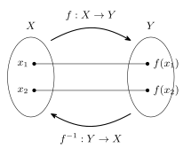
Figure 213: A bijection \(f\) pairs \(x_1\) with \(f(x_1)\) and \(x_2\) with \(f(x_2)\), one arrow each, nothing shared, nothing missed — and so the arrows can be read backwards. The curved arrow above is \(f : X \to Y\); the one below is \(f^{-1} : Y \to X\), the same pairs in the other direction.
Drop either and \(f^{-1}\) is not a function: if \(f\) is not onto, some \(y\) has nowhere to go; if \(f\) is not one-to-one, some \(y\) has two places to go. Both failures are drawn in 2026-09-07-functions-one-to-one-onto-inverse. And the converse holds too:
\[f \text{ has an inverse} \iff f \text{ is a bijection.}\]
Finding the inverse
The onto proof computes it. Proving \(f\) onto means taking an arbitrary \(y\) (or \((a,b)\)) and producing the \(x\) that maps to it, as a formula in \(y\). That formula is \(f^{-1}\). It is a function whether or not \(f\) is one-to-one; one-to-one is what makes it the inverse, by guaranteeing the \(x\) it produces is the only preimage, so that \(f^{-1} \circ f\) is the identity and not merely \(f \circ f^{-1}\).
\(f : \mathbb{R} \times \mathbb{R} \to \mathbb{R} \times \mathbb{R}\), \(f((x,y)) = (y+1, 2x)\) — a bijection (proved in one-to-one-and-onto-functions).
The onto proof took, for \((a,b)\), the candidate \(\left(\frac{b}{2}, a - 1\right)\). So
\[f^{-1} : \mathbb{R} \times \mathbb{R} \to \mathbb{R} \times \mathbb{R}, \qquad f^{-1}((a,b)) = \left(\tfrac{b}{2}, \; a - 1\right), \quad\text{i.e.}\quad f^{-1}((x,y)) = \left(\tfrac{y}{2}, \; x - 1\right).\]
Sense check, both ways: \[f\!\left(f^{-1}((x,y))\right) = f\!\left(\left(\tfrac{y}{2}, x-1\right)\right) = \left((x-1)+1, \; 2 \cdot \tfrac{y}{2}\right) = (x,y),\] \[f^{-1}\!\left(f((x,y))\right) = f^{-1}((y+1, 2x)) = \left(\tfrac{2x}{2}, \; (y+1) - 1\right) = (x,y).\]
In the language of composition-of-functions: \(f \circ f^{-1}\) and \(f^{-1} \circ f\) are both the identity, and checking one of them is the standard way to confirm an inverse has been computed correctly.
For a function given by a formula in one variable the procedure is the same: set \(f(x) = y\), solve for \(x\) in terms of \(y\), and the solution is \(f^{-1}(y)\) — provided the solution is unique and always in the domain, which is what “bijection” guarantees.
The two meanings of \(f^{-1}\)
This is the most common source of wrong answers in this topic.
1. Preimage. If \(f : X \to Y\) is any function and \(A \subseteq Y\), then the inverse image or preimage of \(A\) is \[f^{-1}(A) = \{x \in X : f(x) \in A\}.\] The preimage function is a function \(f^{-1} : \mathcal{P}(Y) \to \mathcal{P}(X)\).
2. Inverse function. If \(f : X \to Y\) is a bijection, then the inverse function of \(f\) is \(f^{-1} : Y \to X\) with $f^{-1}(y) = $ the unique \(x\) such that \(f(x) = y\). The inverse function is a function \(f^{-1} : Y \to X\).
| Takes | Gives | Exists | |
|---|---|---|---|
| preimage \(f^{-1}(A)\) | a subset \(A \subseteq Y\) | a subset of \(X\) | for every function |
| inverse function \(f^{-1}(y)\) | an element \(y \in Y\) | an element of \(X\) | only if \(f\) is a bijection |
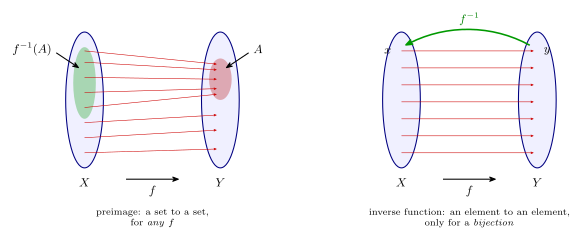
Figure 214: The two meanings side by side. Left: a many-to-one \(f\), with a subset \(A\) of \(Y\) (red) and its preimage \(f^{-1}(A)\) (green) — every \(x\) whose arrow lands in \(A\). This exists for any function, and it is a set. Right: a bijective \(f\), every arrow its own, and the single green arrow \(f^{-1}\) running one element back from \(y\) to \(x\). Same symbol; the first eats sets and the second eats elements.
The braces decide. \(f^{-1}(\{a\})\) has a set inside, so it is a preimage and always means something. \(f^{-1}(a)\) has an element inside, so it is the inverse function and means something only if \(f\) is a bijection.
Worked: reading the braces
\(f : \{1,2,3,4\} \to \{a,b,c\}\), \(f = \{(1,a), (2,a), (3,b), (4,b)\}\).
\(f\) is not one-to-one (\(1, 2 \mapsto a\)) and not onto (\(c\) unreached), so it is not a bijection.
| Statement | Because | |
|---|---|---|
| The inverse function \(f^{-1}\) does not exist. | T | \(f\) is not a bijection |
| \(f^{-1}(\{a\}) = \{1,2\}\). | T | preimage: 1 and 2 map to \(a\), nothing else does |
| \(f^{-1}(a)\) is not defined. | T | \(a\) is an element, so this is the inverse function, which does not exist |
| \(f^{-1}(\{c\}) = \emptyset\). | T | preimage: nothing maps to \(c\), and \(\emptyset\) is a perfectly good answer |
All four are true. The second and third differ only in the braces, and one is a set while the other is undefined.
When \(f\) is a bijection the two meanings agree in the obvious way: \(f^{-1}(\{y\}) = \{f^{-1}(y)\}\), a one-element set whose element is the inverse function’s value. That is the only case in which it is safe to blur them, and even then the types differ.
See also
- one-to-one-and-onto-functions — the two properties a bijection needs, and how to prove them
- composition-of-functions — \(f \circ f^{-1}\) and \(f^{-1} \circ f\)
- symmetric-group — the inverse function as the inverse of an element of a group
- groups — \(f(x) = ax + b\) with \(a \neq 0\) has inverse \(f^{-1}(x) = \frac1a x - \frac{b}{a}\), its inverse in the group of such functions
- functions-on-general-sets — image and preimage, where meaning 1 comes from
- sets-and-set-notation — power sets, which the preimage function maps between
- 2026-09-07-functions-one-to-one-onto-inverse — Lecture 19 · 2026-09-08-composition-of-functions — Lecture 20
- practice-problems — §25
Logical Connectives
Logic is the study of reasoning, and the language of symbolic logic is what lets us analyse ordinary sentences, test arguments for validity, construct proofs for complex arguments, and identify incorrect proofs and common fallacies. This note covers the first layer of that language: statements, the three basic connectives, and the truth tables that define them.
Statements
A statement (or proposition) is a sentence that is either true or false, but not both. Represented by variables \(p, q, r, \dots\)
| Sentence | Statement? | Why |
|---|---|---|
| “6 is odd.” | Yes — and it is false | Definitely one of T/F, and we can say which |
| “It is raining.” | Yes | Which value it takes depends on the circumstances — it could be either — but in any given circumstance it is definitely one or the other |
| “\(x\) is odd.” | No | Its truth depends on the unspecified \(x\), so it has no truth value on its own |
| “Is it raining?” | No | A question is not true or false |
| “She is happy.” | No | Not objectively true or false |
The row worth pausing on is “It is raining.” A sentence does not stop being a statement just because you personally don’t know which value it has. What disqualifies “\(x\) is odd.” is different: it has a free variable, so there is nothing to be true about until \(x\) is fixed. Sentences of that shape are predicates, and the machinery for turning them into statements is quantifiers — see quantified-statements.
Basic connectives
| Connective | Symbol | Alt. symbol |
|---|---|---|
| not | \(\sim\) | \(\neg\) |
| and | \(\land\) | |
| or (inclusive) | \(\lor\) |
\(\sim\) and \(\neg\) are both common symbols for “not”. This course writes \(\sim\), and so does the examination formula page, so that is what these notes use.
\(p \lor q\) is true when \(p\) is true, \(q\) is true, or both (“inclusive or”).
The defining truth tables
These three must be known by heart:
| \(p\) | \(q\) | \(p \land q\) | \(p \lor q\) |
|---|---|---|---|
| T | T | T | T |
| T | F | F | T |
| F | T | F | T |
| F | F | F | F |
| \(p\) | \(\sim p\) |
|---|---|
| T | F |
| F | T |
Inclusive vs exclusive in English
Ordinary English uses “or” both ways:
- “Would you like red or white wine?” — reads as exclusive; you’re expected to pick one.
- “Would you like milk or sugar with your tea?” — reads as inclusive; both is a perfectly good answer.
\(\lor\) is always the inclusive one.
Translating English into symbols
Translating between English and mathematics is difficult, and three English words carry most of that difficulty:
| English | Symbolic | Note |
|---|---|---|
| but | \(\land\) | Carries a contrast in English, none in logic — “it is not cold but it is snowing” is \(\sim p \land q\) |
| neither \(A\) nor \(B\) | \(\sim(A \lor B)\), equivalently \(\sim A \land \sim B\) | “Neither … nor” is the negation of an “or” statement — the De Morgan rewrite is why the two forms agree (see logical-equivalence-laws) |
| or | \(\lor\) | Always inclusive, whatever the English suggests |
Worked. Let \(p\) = “it is cold”, \(q\) = “it is snowing”, \(r\) = “it is sunny”.
| English | Symbolic |
|---|---|
| It is not cold but it is snowing. | \(\sim p \land q\) |
| It is neither snowing nor cold, but it is sunny. | \(\sim(q \lor p) \land r \;\equiv\; (\sim q \,\land\sim p) \land r\) |
and back the other way:
| Symbolic | English |
|---|---|
| \(\sim q \land p\) | It is not snowing and it is cold. |
| \((p \land q) \lor r\) | It is cold and snowing, or it is sunny. (Inclusive — a cold, snowing, sunny day satisfies it.) |
Are “It is not cold but it is snowing” and “It is snowing and it is not cold” equivalent? Yes, by the commutative law: \(\sim p \land q \equiv q \,\land\sim p\). The English word order changes and the meaning does not.
Exclusive or (\(\oplus\))
“One or the other, but not both”, often written XOR:
\[p \oplus q \equiv (p \lor q) \land \sim(p \land q)\]
Laid beside the two inclusive connectives, so the differences are visible in one place:
| \(p\) | \(q\) | \(p \land q\) | \(p \lor q\) | \(p \oplus q\) |
|---|---|---|---|---|
| T | T | T | T | F |
| T | F | F | T | T |
| F | T | F | T | T |
| F | F | F | F | F |
\(\oplus\) is equivalent to neither of them:
\[p \oplus q \;\not\equiv\; p \lor q \qquad\qquad p \oplus q \;\not\equiv\; p \land q\]
\(\oplus\) agrees with \(\lor\) everywhere except the “both” row, and agrees with \(\land\) only on the row where neither holds.
Order of operations
- \(\sim\) first.
- \(\land, \lor\) equal second — parenthesise, else left to right.
\(\to\) and \(\leftrightarrow\) join as an equal third tier; see conditional-statements.
Worked. Take the statement form
\[(p \land q) \lor \sim (r \lor p) \land s\]
Because \(\sim\) binds first, the \(\sim\) takes only \((r \lor p)\); the remaining \(\lor\) and \(\land\) are then resolved left to right. So it means
\[\big((p \land q) \lor (\sim (r \lor p))\big) \land s\]
which is a different statement form from \((p \land q) \lor \big((\sim (r \lor p)) \land s\big)\) — the reading you would get by assuming \(\land\) binds tighter than \(\lor\). In this course they are equal in precedence, so that assumption is wrong here. Write the parentheses.
Truth tables
A truth table shows the truth value of a statement form for all possible truth values of its statement variables. A statement form with \(n\) variables has \(2^n\) rows, where \(n\) counts the distinct letters, not the occurrences.
Take \((p \land q) \land (q \land r)\). Each unique letter is a variable, so there are 3 variables \(p, q, r\) — not 2 and not 4 — and the table has \(2^3 = 8\) rows. The repeated \(q\) does not add one.
Standard truth table form
Construct your truth tables in standard form so that (i) you are sure you have covered all combinations of the truth values of the statement variables, and (ii) it is easy for someone to check your work.
Standard form fixes the row order: the first variable is T for the whole top half and F for the whole bottom half, and each later variable halves the run again, so the last variable alternates T, F every row.
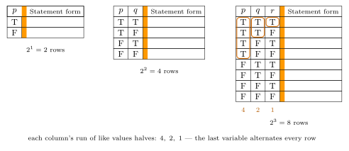
Figure 215: Standard truth table form for one, two and three variables. Each new variable doubles the number of rows and halves the run of like values — 4, 2, 1 for three variables — so the pattern is fixed and completeness is checkable at a glance. The rings mark that pattern on the three-variable table. The narrow amber column separates the variables from the statement-form column.
The four-variable table extends the same pattern: \(p\) runs T for eight rows then F for eight, \(q\) in blocks of four, \(r\) in blocks of two, \(s\) alternating — \(2^4 = 16\) rows.
For how to build the intermediate columns of a compound form, and the convention of numbering them in evaluation order, see the worked table in 2026-07-30-logical-form-and-equivalence.
See also
- logical-equivalence-laws
- conditional-statements
- quantified-statements — what to do with sentences like “\(x\) is odd” that are not statements
- 2026-07-30-logical-form-and-equivalence — Lecture 2, where all of this was introduced
- practice-problems — §1 Logical Form, with full worked solutions
Logical Equivalence & Laws
Two statement forms are logically equivalent (\(\equiv\)) if they have the same truth value for every combination of truth values of their variables — shown via a truth table, or by chaining the laws below. To show two forms are not equivalent (\(\not\equiv\)), exhibit one combination of truth values where they differ.
\(\equiv\) compares statements (like \(=\) compares numbers); it’s not a connective itself. The connective that combines two statements into one is the biconditional \(\leftrightarrow\) — see conditional-statements.
Tautologies and contradictions
A tautology \(\mathbf{t}\) is a statement that is always true. A contradiction \(\mathbf{c}\) is a statement that is always false.
Both are written in bold upright lower case on the formula sheet, and both appear as values inside the laws — \(p \lor \sim p \equiv \mathbf{t}\) produces one, \(p \land \mathbf{t} \equiv p\) consumes one. A chain of laws that reaches \(\mathbf{t}\) or \(\mathbf{c}\) has proved the original form is always true or always false, which is usually the point of the exercise.
Laws of logical equivalence
Provided in the exam. These laws are printed on the MATH1061/MATH7861 Examination Formula Page, so they don’t need memorising. What the exercises ask for is choosing and applying them, and naming the one used at each step. The same page also carries the valid-argument-forms and the set identities of proving-set-properties.
Given statement variables \(p, q, r\), a tautology \(\mathbf{t}\), and a contradiction \(\mathbf{c}\):
| Law | Form 1 | Form 2 |
|---|---|---|
| Commutative | \(p \land q \equiv q \land p\) | \(p \lor q \equiv q \lor p\) |
| Associative | \((p \land q) \land r \equiv p \land (q \land r)\) | \((p \lor q) \lor r \equiv p \lor (q \lor r)\) |
| Distributive | \(p \land (q \lor r) \equiv (p \land q) \lor (p \land r)\) | \(p \lor (q \land r) \equiv (p \lor q) \land (p \lor r)\) |
| Identity | \(p \land \mathbf{t} \equiv p\) | \(p \lor \mathbf{c} \equiv p\) |
| Negation | \(p \lor \sim p \equiv \mathbf{t}\) | \(p \land \sim p \equiv \mathbf{c}\) |
| Double negative | \(\sim(\sim p) \equiv p\) | |
| Idempotent | \(p \land p \equiv p\) | \(p \lor p \equiv p\) |
| Universal bound | \(p \lor \mathbf{t} \equiv \mathbf{t}\) | \(p \land \mathbf{c} \equiv \mathbf{c}\) |
| De Morgan’s | \(\sim(p \land q) \equiv \sim p \lor \sim q\) | \(\sim(p \lor q) \equiv \sim p \land \sim q\) |
| Absorption | \(p \lor (p \land q) \equiv p\) | \(p \land (p \lor q) \equiv p\) |
| Negations of \(\mathbf{t}\)/\(\mathbf{c}\) | \(\sim \mathbf{t} \equiv \mathbf{c}\) | \(\sim \mathbf{c} \equiv \mathbf{t}\) |
De Morgan’s Laws are especially important for negating “and”/“or” statements — e.g. the negation of “5 is divisible by 2 and 6 is divisible by 2” is “5 is not divisible by 2 or 6 is not divisible by 2”. Note what changes: the connective flips from and to or, and both halves get negated. Negating only one half, or leaving the connective alone, is the standard error.
How to write a law chain
The layout expected in your own work:
- the first line is the starting expression, on its own;
- every later line begins with \(\equiv\), vertically aligned down the page;
- the name of the law used to get there sits in its own right-hand column on that line.
Two or more laws may be cited on one line if they act on the same step (e.g. “by De Morgan’s law and the double negative law”). Name a law on every line that changes the expression. The one kind of line that goes unnamed is a pure re-labelling that asserts nothing new, like the “where \(r = (p \,\land\sim q)\)” line in the first worked example below.
Treat a compound expression as a single letter
The laws are stated for variables \(p, q, r\), but they hold with any statement form substituted in. Spotting that turns a long expression into a short one:
\[(p \,\land\sim q) \;\land\; \sim(p \,\land\sim q)\]
is \(r \,\land\sim r\) with \(r = (p \,\land\sim q)\), so the negation law applies directly and it is \(\mathbf{c}\). This is exactly the move in the first worked example below.
Worked: reaching a contradiction
Show that \((p \,\land\sim q) \land (\sim p \lor q) \equiv \mathbf{c}\).
\[ \begin{aligned} (p \,\land\sim q) \land (\sim p \lor q) &\equiv (p \,\land\sim q) \;\land\; \sim(p \,\land\sim q) && \text{by De Morgan's law and the double negative law} \\ &\equiv r \,\land\sim r \quad \text{where } r = (p \,\land\sim q) \\ &\equiv \mathbf{c} && \text{by the negation law} \end{aligned} \]
The whole proof is the first line: recognising that \(\sim p \lor q\) is \(\sim(p \,\land\sim q)\) in disguise. Read De Morgan’s backwards — \(\sim p \lor q \equiv \sim p \,\lor\sim(\sim q) \equiv \sim(p \,\land\sim q)\) — and the two conjuncts are a statement and its own negation.
Worked: absorbing a conjunction
Show that \(\sim p \lor (p \land q) \equiv \sim p \lor q\).
\[ \begin{aligned} \sim p \lor (p \land q) &\equiv (\sim p \lor p) \land (\sim p \lor q) && \text{by the distributive law} \\ &\equiv \mathbf{t} \land (\sim p \lor q) && \text{by the negation law} \\ &\equiv \sim p \lor q && \text{by the identity law} \end{aligned} \]
The pattern distribute, collapse the tautology or contradiction, drop it with the identity law is the most common three-step shape in this topic, and it recurs in both routes below.
Worked: two routes to the same answer
Show that \(\sim\big((\sim p \land q) \lor (\sim p \,\land\sim q)\big) \equiv p\).
There is no unique chain. Here are two, and both are complete proofs:
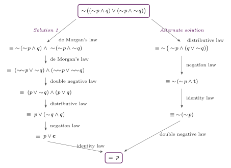
Figure 216: The same equivalence proved two ways. Starting from the same expression and ending at the same p, the left route pushes the negation inward with De Morgan’s first and takes six steps; the right route factors out the common ~p with the distributive law first and takes four. Every edge names the law that licenses it — that naming is what the chain is for.
Neither route is “the” answer, and nothing turns on finding the short one. What matters is that every line follows from the one above by a named law. The shorter route is found by looking for a common factor before doing anything else: both disjuncts inside the brackets contain \(\sim p\), so the distributive law pulls it out and the rest collapses.
The same equivalence can also be established with a truth table — see the worked table in 2026-07-30-logical-form-and-equivalence, where the column for \(\sim\big((\sim p \land q) \lor (\sim p \,\land\sim q)\big)\) comes out identical to the column for \(p\).
Showing two forms are not equivalent
To show \(\not\equiv\) you do not need a full truth table. Find one assignment of truth values on which the two forms disagree, and say what each evaluates to.
Worked. Show that \(\sim(p \lor q) \;\not\equiv\; \sim p \lor \sim q\).
Take \(p\) false and \(q\) true. Then
- LHS: \(p \lor q\) is \(\mathrm{F} \lor \mathrm{T} = \mathrm{T}\), so \(\sim(p \lor q)\) is false.
- RHS: \(\sim p \,\lor\sim q\) is \(\mathrm{T} \lor \mathrm{F} = \mathrm{T}\), so it is true.
One row on which they differ is a complete disproof, so the two forms are not logically equivalent.
The correct partner for \(\sim(p \lor q)\) is of course \(\sim p \,\land\sim q\) — this is precisely the De Morgan trap of changing the sign but not the connective.
See also
- logical-connectives
- conditional-statements
- formula-sheet — what else is provided in the exam, and what is not
- proving-set-properties — the same eleven laws as set identities, and the two set-equality proof methods built on them
- 2026-07-30-logical-form-and-equivalence — Lecture 2, where these laws were introduced and applied
- practice-problems — §2 Logical Equivalence, with full worked solutions
Diagram and Notation Conventions
The house style for every figure, symbol and proof layout in MATH1061 — read off the course’s own lecture slides rather than assumed. This is the authority any new diagram for this course is checked against. Where the source does not settle something, that is said so explicitly rather than filled in.
What was read
Everything the course ships in the anchor set, in full: all 176 slide pages across the 18 lecture decks (L01–L18), plus the 1-page examination formula sheet. No sampling — the whole corpus was viewed as rendered images so the drawings, ink colours and box shapes were seen, not inferred from extracted text.
Citations below use L07 p2 = PDF page 2 of math1061-lecture-07-…pdf. Two decks have a page-label offset worth knowing: L03 p2–p3 carry the printed header Lecture 2, and L17 p9–p10 carry the printed header Lecture 18. PDF page position is what is cited.
The course ships one written reference — the MATH1061/MATH7861 Examination Formula Page. It is a genuine notation authority (it fixes ∼, ≡, bold t/c, Aᶜ, ∴, A − B, and the numbering of the set identities), but it is not a drawing guide: it says nothing about figures, colour, layout or symbol shape. Everything in the Diagrams section below is inferred from the decks alone.
Only 18 of the course’s 36 lectures exist in this set (L19–L36 — one-to-one/onto functions, composition, cardinality, relations, equivalence and partial orders, groups, fields, counting, probability, pigeonhole, graph theory, walks, matrix representations, trees — are absent). Conventions for those topics are unestablished; see the last section.
Provenance: two lecturers, one template
The course is split between two lecturers (L01 p12, course schedule): Sara Davies takes L01–L09 and L18–L26; Katie Clinch takes L10–L17 and L27–L36. Both use the same slide frame, but their annotation habits and some box conventions differ. Where they diverge it is recorded under Inconsistencies, not resolved.
Textbook lineage
The recommended text is Susanna Epp, Discrete Mathematics with Applications, 4th or 5th (metric) edition (L01 p3, with the cover image on the slide). It is cited repeatedly by page for statements and exercises — L14 p7 (“Q27 on page 279 of Epp”), L14 p8 (“Q31 on page 279”), L16 p12 (“page 310 (in 4th edition) or page 346 (in 5th edition)”), L18 p8 (“pages 419-421 (ed. 5) or pages 378-380 (ed. 4)”).
Important qualification: no slide anywhere carries a caption naming a textbook as the source of a figure. The Epp lineage is real for wording and content — the logical-equivalence names, the valid-argument-form names and the twelve numbered set identities are Epp’s — but it is not documented evidence for any drawing style. Do not cite Epp as a figure source.
Slide frame and page furniture
| Element | Convention | Evidence | Holds? |
|---|---|---|---|
| Header band | Page 1 of each deck: MATH1061/MATH7861 Discrete Mathematics Semester 2, 2026 at far left, Lecture N – Title at far right. Later pages: right-hand lecture label only. A full-width thin black rule sits beneath. |
L02 p1 vs L02 p2; identical in every deck L02–L18 |
Every deck except L01, which has UQ-branded title slides |
| Pre-work box | A purple rounded-rectangle box, top right of page 1, headed Pre-work video: / Pre-work videos: in bold, listing Video NNN Title with three-digit zero-padded numbers |
L02 p1, L03 p1, L05 p1, L07 p1, L10 p1, L13 p1, L16 p1, L18 p1 |
All 17 decks L02–L18 — the single most consistent element in the course |
| Learning goals | Bold Learning Goals heading, numbered list 1. 2. 3. |
L02 p1 … L18 p1 |
Every deck L02–L18 (L07 p1 uses an unnumbered list — the one exception) |
| Student Q&A | Bold blue heading Student questions and comments: (or Student questions:), questions in blue, answers in red |
L02 p1, L04 p1, L06 p1, L08 p1, L11 p1, L12 p1, L15 p1, L18 p1 |
Every deck L02–L18 |
| Activities | Bold Activity N: restarting at 1 each lecture; pre-class items as Q1 from the pre-class questions; Clinch decks add Poll question N: |
L02 p3, L07 p5, L12 p2, L17 p3 |
Throughout |
Figures are never numbered and never labelled “Figure”. When a caption exists it sits centred directly beneath the drawing, either as the mathematical expression it depicts ((A − B), L18 p2) or as a short prose verdict (not a function / a function, L18 p9).
Colour
Printed colour on slides
- Red = the thing you must not get wrong. Warnings, answers to student questions, “IMPORTANT NOTE”, “Take care with notation!”, “WARNING”.
L01 p4(“hurdles”),L02 p1,L08 p2(“WARNING”),L10 p1(“IMPORTANT NOTE”),L11 p4(“Take care with notation!”),L17 p2(“Warning!!!!”),L17 p9. Holds in both lecturers’ decks, all semester. - Blue = student voice and explanatory gloss. Student questions (
L02 p1onward, universal) and, in Clinch’s decks, a plain-English restatement placed directly beneath a formal condition written in red —L12 p3(d|a and d|bin red, “d is a divisor of both a and b” in blue below it),L12 p4(same pattern for lcm). That paired red-above/blue-below idiom is specific and recurs. - Colour as correspondence, not meaning. Where two expressions must be matched piece-by-piece, matching pieces are given matching colours.
L03 p9(a three-row table wherea ↔︎ b,a if and only if b,b is necessary and sufficient for aare colour-aligned column by column),L06 p6(quantifier negation, below),L11 p3(quotient in red above q, remainder in red above r, and the same two colours on the worked examples). This is the one place colour genuinely carries information. - Pastel highlight capsules (yellow, green, blue, pink, orange) mark the single expression being tracked through a calculation — it keeps its capsule colour as it moves line to line. Heavily used by Clinch:
L11 p3,L12 p6,L13 p6,L14 p3,L16 p5,L17 p5. Rare in Davies’s decks.
Annotation ink (live handwriting)
Both lecturers annotate over the slides in ink. Blue is the predominant ink for the main worked solution — L01 p13, L02 p7, L04 p4, L07 p4, L08 p5, L10 p5, L13 p7, L16 p7, L18 p3. Other colours (green, red, purple, orange, teal) are layered over it for justifications, second solutions, and circling.
Be honest about what ink colour means: mostly, nothing fixed. It separates successive layers of annotation for legibility, and rotates. The two places it is systematic:
- Correspondence — e.g.
L02 p6, where each intermediate truth-table column is written in its own colour and numbered ①②③ in that colour to show evaluation order, with the final column ringed and labelled “final answer”. - Verdict marks — a green circled
Tand a red circledFfor true/false answers:L05 p7,L05 p8,L06 p4. Green tick / red cross for correct/incorrect options:L06 p3,L09 p4,L16 p2.
Boxes and callouts
| Shape | Meaning | Evidence | Holds? |
|---|---|---|---|
| Purple rounded rectangle | A named, quotable object: definition, Fact, Lemma, Theorem — and the pre-work video box | L07 p1 (the six definitions), L07 p2 (two Facts), L08 p2, L09 p6 (Fact + Lemma), L10 p6, L10 p7 (Unique Factorisation Theorem), L10 p9, L10 p12, L11 p3 (Quotient-Remainder Theorem), L11 p7, L11 p8 |
Strong: both lecturers, L07 through L12 |
| Plain thin black rectangle | A structural panel — a proof skeleton, or a two-way comparison | L07 p3, L08 p3, L09 p2 (the four proof-method skeletons), L11 p3 (“2 equivalent ways of defining…”) |
Consistent where it appears |
| Red rectangle | Davies: a fact that must be memorised or a warning. Clinch: a numbered step caption or a named principle | L02 p8 (De Morgan’s laws), L03 p4, L03 p9, L04 p1 (“Recall:”), L01 p4; and L10 p6 (margin commentary), L12 p10 (steps 1/2/3), L14 p6 (Well-ordering Principle) |
Both uses recur; see Inconsistencies |
| Margin callout with arrow | A red-outlined box in the right margin, with a red arrow to the exact proof line it explains, and a purple ★ at the anchor point | L10 p6 (two callouts, two arrows, two stars) |
Seen once — extrapolating from a single instance |
| Hand-drawn cloud | An aside or a menu of options: “What type of proof will work?” with ✓/✗ against each method | L09 p4, L09 p5, L09 p6, L09 p7; L14 p3 |
Four consecutive slides in L09, once in L14 |
Logic notation
Fixed by the formula sheet and used unchanged in every deck:
| Symbol | Reading | Note |
|---|---|---|
∼ p |
not p | The course symbol is the tilde ∼, not ¬. L02 p1 answers this directly: “some common symbols for not include ∼ and ¬” — both exist, this course writes ∼. Used in every deck and on the formula sheet |
p ∧ q, p ∨ q |
and, or | ∨ is inclusive or; exclusive or is ⊕ (L02 p5) |
p → q |
if p then q | L03 p1; defined as ∼ p ∨ q |
p ↔︎ q |
if and only if | A connective that combines statements |
p ≡ q, p ≢ q |
logically equivalent / not | A relation that compares statements |
| t, c | tautology, contradiction | Bold upright, lower case. Formula sheet; L02 p9 |
∴ |
therefore | Prefixes the conclusion of an argument |
↔︎ versus ≡ is stated explicitly and must not be blurred (L03 p7): “The biconditional (↔︎) is a conjunction used to combine statements (similar to +, -, x, ÷ … with numbers). Logical equivalence (≡) is used when comparing two statements (similar to = with numbers).”
Precedence (L02 p5, extended at L03 p7): ∼ first; ∧ and ∨ equal second; → and ↔︎ equal third; within a tier, work left to right — “but parentheses should always be used to avoid confusion.”
Statement variables are lower-case italic p, q, r. When a problem is in English, the letters are chosen as mnemonics of the English phrase: w = wages, b = buying, d = depression (L04 p4); q = queued, s = sent to the buffer (L05 p2).
Truth tables
The course calls this “standard truth table form” and requires it (L02 p4): “You should construct your truth tables in standard form so that you are sure you have covered all combinations … and it is easy for someone to check your work.”
- Values are the single upright capitals
TandF— never 1/0, never True/False. Universal:L02 p4,L03 p1,L04 p5,L06 p2,L07 p3,L09 p2. - 2ⁿ rows for n variables, in a fixed order: the first variable is
Tfor the whole top half thenFfor the whole bottom half; each subsequent variable halves again; the last variable alternatesT,Fevery row. Shown for n = 1, 2, 3, 4 side by side atL02 p4. - A narrow solid-filled amber/orange column separates the input block from the compound-form block.
L02 p4(after the variable columns, before “Statement form”);L04 p5(after the variables and their simple negations, before the premise and conclusion columns). Two instances, both lecturers’ style aside — treat as the course’s own table furniture. - Header row typeset in red italic maths (
p,q,p → q), body values in black upright.L03 p1,L03 p4,L04 p1,L04 p2,L04 p5,L07 p3,L08 p3,L09 p2. Consistent throughout Davies’s decks; Clinch draws no printed truth tables. - Full ruled grid — every cell bordered.
- When built by hand, columns are added left to right in evaluation order and numbered ①②③ beneath, each in its own ink colour, with the answer column ringed.
L02 p6,L03 p2. AtL03 p2the two columns that must match are marked with a✳beneath and the verdict written out: “Starred columns are identical so ∼((∼p∧q) ∨ (∼p∧∼q)) ≡ p”.
Arguments and inference proofs
Argument form (formula sheet; L04 p2, L04 p3, L04 p6, L05 p2, L05 p4): premises stacked one per line, left-aligned; the conclusion on the last line prefixed by ∴. No horizontal rule above the conclusion. Premises are numbered 1. 2. 3. and the ∴ line is left unnumbered.
Rules-of-inference proof (L04 p6, L04 p7, L05 p4): numbered lines down the left, the derived statement in the middle, and the justification in its own right-hand column, phrased as from ② by contraposition, from ① & ④ by transitivity, by double negative law, by definition of →. The annotation at L04 p6 is emphatic: “must write explanations!”.
Equivalence-law chains (L02 p10, L03 p8, L18 p5, L18 p7): first line is the starting expression; every subsequent line begins with ≡ (or = for sets), vertically aligned, with the named law in a right-hand column — by de Morgan's law, by the negation law, by identity law. For set identities the numbered law from the formula sheet is cited: by set diff law (12), by de Morgan (9b), dist. law (3b), complement law (5b), identity law (4a) (L18 p7).
Biconditional proofs are marked by direction: ⇒ and ⇐ label the two halves (L12 p8). Two named methods, with a stated preference — Method 1, prove each direction separately, is annotated “recommended method”; Method 2, an iff chain, is annotated “Be careful! Quicker method but easy to make a logical error” (L12 p8, L12 p9).
Quantifiers
∀x ∈ D, P(x)— universal, comma after the domain.∃x ∈ D such that P(x)— existential, the words “such that”, abbreviateds.t.(L06 p1,L05 p7).- Both established at
L05 p5and used unchanged throughL08 p1,L17 p3. ∈reads “is an element of” / “belongs to”;∉“is not an element of” (L05 p5).- Negation rules, stated as displayed equivalences at
L08 p1:∼(∃x ∈ D such that P(x)) ≡ ∀x ∈ D, ∼P(x)and∼(∀x ∈ D, P(x)) ≡ ∃x ∈ D such that ∼P(x).
Number sets
Blackboard-bold, established at L05 p1 and used unchanged to the end: ℝ, ℚ, ℤ, ℕ.
Irrational numbers are written ℚ̄ — ℚ with an overbar (L05 p1, L09 p1, L09 p3, L09 p6). Not ℝ∖ℚ; the equality ℝ∖ℚ = ℚ̄ is written by hand at L09 p1 as a gloss, but the barred form is what the printed slides use.
Restrictions are written as superscripts on the set symbol, in italic, not as subscripts and not as prose:
ℤ⁺ ℤ^even ℤ^odd ℤ^nonneg ℤ^prime ℤ^composite ℤ^{>1} ℤ^{≥2} ℤ^{≤1} ℤ⁻
Evidence: L05 p1 (ℤ⁺, ℤ^even, ℤ^nonneg), L07 p2 (ℤ^even, ℤ^odd, ℤ^prime, ℤ^composite, ℤ^{≤1}, ℤ^{>1}), L07 p6 (ℤ^{≥2}), L10 p12 (ℤ^{≥2}), L17 p10 (ℤ⁺, ℤ⁻). Strong and semester-long.
Proof layout
The four methods each have a fixed printed skeleton, given verbatim on a repeated slide (L07 p3, L08 p3, L09 p2 — the same panel, grown one box at a time as methods are introduced). Reproduce these wordings:
- Direct proof —
Let x ∈ D and suppose P(x).…Hence Q(x).□ - Disproof by counterexample —
Let x = ⋯. Then x ∈ D and P(x) is true.However, Q(x) is false.So x is a counterexample and the statement is false. - Proof by contradiction —
Suppose the negation of ∀x ∈ D, P(x) → Q(x) is true.That is, suppose ∃x ∈ D such that P(x) is true but Q(x) is false.…Hence something that is obviously wrong…This is a contradiction, and we conclude that … is true.□ - Proof by contraposition —
We prove the contrapositive of ∀x ∈ D, P(x) → Q(x), namely that ∀x ∈ D, ∼Q(x) → ∼P(x).Let x ∈ D and suppose ∼Q(x).…Hence, ∼P(x).□
Each box carries a red caption directly beneath it saying what it establishes: Shows the statement is true. / Shows the statement is false. (L07 p3, L08 p3).
Other layout facts:
Proof:label, then the hypothesis line, then the working with=signs vertically aligned in a column, then aHence/Thus/Soconclusion.L07 p4,L07 p5,L08 p5,L09 p3,L10 p5.- Method comparison is a two-column layout with bold centred headings —
Direct Proofleft,Proof by contradictionright (L08 p5,L08 p6);Proof SMI/Proof MI/Proof WOP(L14 p7,L14 p8). Without loss of generality, spelled out then abbreviatedWLOG(L08 p8,L09 p5).- Case splits are labelled
Case 1:/Case 2:(L10 p6,L10 p12,L14 p5). - Every proof unfolds definitions. The six definitions in the purple box at
L07 p1/L08 p2are stated as biconditionals using↔︎— e.g.n is an even integer ↔︎ n = 2k for some integer k,d|n ↔︎ d ≠ 0 and n = dk for some integer k— because they are used in both directions. - Introduce a new variable for each new existential. Annotated explicitly at
L08 p6: “use a new variable!” wherem = 2k+1is followed byn = 2ℓ+1.
End-of-proof mark
Printed proofs end with an open square □: L07 p3, L07 p4, L08 p3, L09 p2, L10 p6, L10 p11, L10 p12.
Handwritten proofs end with either a hand-drawn open square (L07 p5, L08 p8, L09 p4, L09 p5, L09 p6) or a double slash // (L10 p5, L11 p6, L13 p7, L13 p9, L14 p10, L15 p5, L16 p7, L18 p3, L18 p7). At L11 p6 the lecturer writes an explicit legend of the acceptable marks: // or □ ▪ QED. Treat all four as sanctioned.
Contradiction mark
Davies writes (⇒⇐) — two arrows meeting — inline at the point the contradiction lands: L08 p3, L08 p5, L08 p6, L08 p7, L08 p8, L09 p6. Clinch instead uses a small crossed glyph ⨳ inline, e.g. “(proof by ⨳)” for “proof by contradiction” (L14 p6, twice). See Inconsistencies.
Induction
The named-step skeleton is fixed and printed identically in five separate proofs:
Proof:  Let P(n) be the predicate  ⟨statement⟩.
Basis step:        ⟨verify P(a)⟩ … so P(a) is true.
Inductive step:    Prove that ∀k ∈ ℤ with k ≥ a, if P(k) is true, then P(k+1) is true.
Inductive hypothesis:  Suppose that k ≥ a is an integer and that P(k) is true.
        LHS of P(k+1):  ⟨chain of = with the RHS reached⟩
        Therefore P(k+1) is true.
Therefore, by ⟨PMI / SMI⟩, ⟨statement⟩ for each integer n ≥ a.
Evidence: L13 p6, L13 p8, L14 p3, L14 p7, L16 p6, L16 p8, L16 p10. Step labels are printed in blue at L13 p6 and in red at L14 p3/L14 p7.
LHS/RHSare the standard abbreviations, and the two sides are named and worked separately:LHS of P(1): …RHS of P(1): …(L13 p6,L13 p7,L16 p7).- The step where the hypothesis is used is annotated
(by the inductive hypothesis)on the same line (L13 p6,L13 p7,L14 p3). - Slides ask for the steps to be named: “It is a good idea to list these explicitly in your proofs to help the reader to follow the proof” (
L13 p1). - Multiple base cases are listed one per line when strong induction needs them (
L14 p4,L15 p8).
Number-theory notation
- Divides:
d | n. Does not divide:d ∤ n(slashed bar).L05 p7,L07 p1,L10 p1,L10 p10,L14 p8. - Equivalent phrasings given at
L10 p1: d divides n, d is a divisor of n, d is a factor of n, n is a multiple of d. n mod d = r(uprightmodas a binary operator, no brackets) versusm ≡ n (mod d)(congruence,(mod d)bracketed after the statement). These are different things and the course flags it twice under a red headingTake care with notation!—L11 p3,L11 p4, recappedL12 p2.gcd(a, b)andlcm(a, b), lower case, upright roman (L12 p3,L12 p4). AtL12 p3the alternativehcf(a,b)is written and then struck through — it is not this course’s name.- Floor
⌊x⌋and ceiling⌈x⌉(L11 p2). - Standard factored form:
n = p₁^{e₁} p₂^{e₂} ⋯ p_k^{e_k}with the primes in increasing orderp₁ < p₂ < ⋯ < p_k(L10 p7, annotated “increasing” atL10 p8). - Multiplication is a centred dot
·in printed slides:2 · 3 · 5 · 7 · 11 ⋯ p(L10 p11),5859 = 1232 · 4 + 931(L12 p6),2 · 100 + 5 · 10 + 4 · 1(L11 p8),3 · 1 + 2(L13 p6).
Sequences, sums and recurrences
- Summation
Σwithi = mbelow andnabove; index lettersi,j,k; change of variable written asj = i + 1(L13 p3,L13 p4,L13 p6). - A recursive definition of a sequence requires two named parts: a recurrence relation and initial conditions (
L15 p3,L16 p7,L16 p9). - A recursive definition of a set requires three named parts: Base, Recursion, Restriction — always in that order, with the Restriction worded “Nothing is in B other than objects defined by the Base and the Recursion” (
L15 p6,L15 p7). - Verifying a guessed explicit formula has two named methods: Method 1 (check the initial conditions and the recurrence relation — annotated “quicker”) and Method 2 (prove it by induction — annotated “rigorous”).
L16 p4, used atL16 p5–L16 p10. n!with0! = 1by definition (L15 p5).
Set-theory notation
| Notation | Meaning | Evidence |
|---|---|---|
x ∈ A |
is an element of | L17 p1 |
A ⊆ B |
is a subset of | L17 p1, L17 p3 |
A ⊂ B |
is a proper subset of (⊆ and there is an element of B not in A) | L17 p3 — the course does use ⊂ strictly for proper |
A ∩ B, A ∪ B |
intersection, union; indexed forms ⋃_{i=1}^{3} Aᵢ, ⋂_{i=1}^{3} Aᵢ |
L17 p1, L17 p6 |
A − B |
set difference; A \ B is stated to be equally acceptable |
L17 p1 — answered directly: “Yes. A − B can be written as A \ B” |
Aᶜ |
complement, superscript c |
L17 p1, L18 p1, formula sheet |
𝒫(A) |
power set, calligraphic script P |
L17 p1, L17 p7, L17 p8 |
A × B |
Cartesian product; ℝ × ℝ also written ℝ² |
L17 p1, L17 p9 |
∅ |
empty set, also written { } |
L17 p5 |
\|A\| |
cardinality | L17 p7, L17 p9 |
{n ∈ ℤ \| n ≡ 2 (mod 8)} |
set-builder with a vertical bar | L17 p3, L18 p2 |
[a, b] |
closed interval {x ∈ ℝ \| a ≤ x ≤ b} |
L17 p6 |
Sets take capital italic letters (A, B, C, S, T, D, E, R, X, Y), the universal set is U, elements take lower case (x, y, t). L17 p3, L18 p1, L18 p6.
The ∈ / ⊆ distinction is the course’s flagged trap — a red Warning!!!! at L17 p2 and the first learning goal of both L17 and L18. 2 ≠ {2} (L17 p2); ℤ ∈ ℚ is false, ℤ ⊆ ℚ is true (L17 p1, L17 p2).
Proof of set statements has three named methods (L18 p4): the element method, using the laws of logical equivalence, and using set identities (citing the formula sheet’s numbering, as above).
Functions (L18 p9–L18 p11): f: X → Y; f ⊆ X × Y such that for each x ∈ X there is a unique y ∈ Y with (x, y) ∈ f. Domain X, co-domain Y (hyphenated in print), range f(X) = {f(x) : x ∈ X}. Image of a subset f(A); inverse image or preimage f⁻¹(B) — both words are given as correct.
Diagrams
This is what the decks actually draw. Nine idioms recur; everything else is a one-off and is labelled as such.
1. Nested closed curves for containment (Euler style)
Number systems are drawn as concentric plain closed curves with each label written inside its own region — ℚ: rational numbers outermost, containing ℤ: integers, containing ℕ: natural numbers; ℝ labelled above the frame, ℚ̄: irrational numbers in a separate adjacent panel. Thin blue rule dividing the two panels; curves thin black; no shading; no element dots. L05 p1. Seen once for number systems, but the same nested-oval idiom recurs for subsets at L17 p3 and L18 p3, so the shape convention is safe — the specific number-system figure is not.
2. Rectangle partitions
A plain rectangle with a thin blue/teal outline stands for the ambient set; thin internal straight lines split it into disjoint parts; each part is labelled in red italic with its superscript-qualified name; the ambient set’s own label sits above and outside the top-left corner. Two instances on one page: ℤ split into ℤ^even | ℤ^odd, and ℤ split into ℤ^{≤1} | ℤ^prime / ℤ^composite. L07 p2. Seen on one page only — but it is the course’s only printed partition figure, and it is the natural pairing with the superscript set notation above.
3. Two-circle Venn diagrams
- Exactly two circles of equal radius, overlapping, drawn side by side in a horizontal row; thin black outline; labels
AandBplaced inside each circle near its top outer edge. - The region being denoted is filled solid grey. The undecorated pair is drawn first, unshaded, as the reference.
- The expression it depicts is the caption, centred directly beneath —
(A − B),(B − A). L18 p2. Three diagrams in a row.- Hand-drawn variant at
L18 p3: a rectangle for the universe with red diagonal hatching over the complement region, withA(green) insideB(green outline) inside it.
Critical rule, stated by the course itself: at L18 p2 a hand annotation brackets all three Venn diagrams and writes “not a proof!”. A Venn diagram in this course illustrates a set statement; it never discharges one. Proofs go through the element method, the laws of logical equivalence, or the set identities (L18 p4).
4. Small icon strip for set relations
A row of thumbnail two-set diagrams, one per notation, aligned under the list of symbols they gloss: set A drawn as a green ellipse, set B as a pale blue/grey ellipse; an element as a small filled dot; the operation’s region filled or hatched in blue. L17 p1 (the full strip: x ∈ A, A ⊆ B, A ⊂ B, A ∩ B, A ∪ B, A − B, and A = B drawn as coincident ellipses). Repeated as single icons at L17 p3, L17 p4, L17 p6. The green-A / grey-B colour pairing holds across all five appearances.
5. Function arrow diagrams (bipartite)
- Two vertical ellipses side by side: the domain
Xon the left, the co-domainYon the right, each labelled beneath the ellipse in blue. - Elements are labelled dots stacked vertically inside each ellipse.
- Each element of
Xis joined to its image by a straight blue line segment. Flow is left to right. - A subset under discussion is marked by a translucent coloured blob drawn around the relevant dots, labelled just outside in the matching colour with its expression (
f({2,3}),f⁻¹({1}),f({1})). L18 p11— four diagrams on the page, all hand-drawn, all following this arrangement.
6. Cartesian-plane graphs
Axes as thin double-headed arrows crossing at the origin; the y label at the top of the vertical axis and the x label at the right of the horizontal axis, both immediately beside the arrowhead; the curve in blue; marked points as filled dots labelled with their coordinate pair (0,1), (5,11); a prose caption centred beneath (Plot of the function y = 2x + 1., not a function, a function). The vertical line test is shown as a red vertical line crossing the curve twice. L18 p9 — three panels in a row.
7. Number lines
Drawn as a horizontal line with an arrowhead at each end, evenly spaced tick marks, integer labels beneath the ticks, and marked points or brackets above the line. L11 p2 (two of them: the real line from −5 to 4 for floor/ceiling, and a minimal one showing only k and k+1 with k + ½ between); L17 p6 (interval [a,b] drawn above the line with filled dots at the closed endpoints, the axis labelled ℝ at the right end).
8. Colour-coded correspondence diagrams
The single most information-dense idiom in the course. At L06 p6, the negation of a two-quantifier statement is shown as two copies of the same statement schema stacked one above the other and horizontally aligned part-for-part, with each corresponding pair of parts underlined in its own colour and joined by a double-headed arrow of that colour:
- red:
∀x ∈ X↔︎∃x ∈ X such that - green:
∃y ∈ Y such that↔︎∀y ∈ Y, - cyan:
P(x,y)↔︎∼P(x,y) - a purple curved double-headed arrow spanning both rows, labelled
negation
Seen once, but it is the canonical figure for the topic. The same alignment-plus-colour technique without arrows appears at L03 p9 and L12 p3.
9. Algorithm and process cascades
- Euclidean algorithm (
L12 p6): the successive equationsa = bq + rstacked vertically down the left; each numeral wrapped in a pastel capsule, and each number keeps the same capsule colour as it migrates frombtoaandrtobon the next line; red diagonal arrows trace those two migrations; a parallel right-hand column carries the matchinggcd(a,b) = gcd(b,r)chain with the same capsule colours. Colour here is pure identity-tracking. - Sequence hops (
L16 p2,L16 p3,L15 p5): terms written in a horizontal row, short curved arrows above or below each gap, labelled with the operation (+3,×3,× −1). - Recursive-construction tree (
L15 p6): rootεat the left, branches as plain straight segments fanning rightwards, node labels at the branch tips, no arrowheads on the branches. The separate derivation chain uses arrows with the rule name written above:ε --1--> 1 --1--> 11 --01--> 1101(L15 p7). - State sequences (
L16 p11, Tower of Hanoi): three vertical blue pegs on a base line; discs as short red horizontal bars, widest at the bottom; each state enclosed in a plain black rectangle; states run left to right; green curved arrows between states labelled with the move count (m_{n-1},1,m_{n-1}). - Partitions of a set as coloured blobs (
L17 p10): irregular non-overlapping closed curves in distinct colours, each containing dots, each labelled just outside in its own colour (A₁green,A₂red,A₃yellow,A₄blue). On the same page a number line is partitioned instead by weaving highlighter stripes — pink forS, green forT— over the tick labels.
Tables
- Full ruled grid, header row present.
- Truth tables as described above.
- Comparison tables put the item varying across the top and the cases down the side, with
T/Fin the cells (L06 p2: three quantified statements across, three setsSdown). - Material reproduced from the examination formula sheet is pasted as an image and therefore appears in serif LaTeX type, visually distinct from the sans-serif slide body:
L02 p9(Logical Equivalences),L04 p3(Valid Argument Forms),L18 p6(Set Identities). If reproducing one of those tables, reproduce the formula sheet’s own wording and numbering.
Inconsistencies
The course does these things more than one way. Both readings are recorded; no winner is picked. A decision is needed before any new figure fixes one.
End-of-proof mark. Printed proofs use
□(L07 p3,L10 p11). Handwritten proofs use a hand-drawn square (L09 p4) or//(L13 p7,L18 p7). AtL11 p6the lecturer offers all of//,□,▪andQEDas equivalent. Clinch’s printed induction proofs (L14 p7,L16 p6) end with a concluding sentence and no mark at all. Four options, all sanctioned. Decide.Contradiction mark. Davies writes
(⇒⇐)(L08 p3,L08 p5,L08 p6,L08 p7,L08 p8,L09 p6). Clinch writes a crossed glyph⨳and uses it as a noun — “(proof by ⨳)” (L14 p6, two occurrences on one page). Decide.Name of the induction principle. Within four decks: “by the principle of mathematical induction” (
L13 p6), “by PMI” (L13 p8,L16 p12), “by MI” (L16 p10), “by SMI” (L14 p5,L16 p8), “by PSMI” (L14 p3,L14 p7). PMI/MI and SMI/PSMI are used for the same two principles in the same lecturer’s decks. Decide.Sequence delimiters. Printed:
{bₙ}_{n≥0}(L13 p2),{aₙ}_{n≥1}(L15 p3), and barea₀, a₁, a₂, …(L14 p3,L16 p2). Handwritten on the same slide (L13 p1):(aₙ)_{n≥0}and{aₙ}_{n=1}^{∞}. Four forms. Decide.Set-builder separator. Vertical bar in
{n ∈ ℤ | n ≡ 2 (mod 8)}(L17 p3),{(x,y)|x ∈ ℝ and y ∈ ℝ}(L18 p9); colon inf = {(x,y) ∈ ℝ × ℝ : y = 2x + 1}(L18 p9, same page),f⁻¹(B) = {x ∈ X : f(x) ∈ B}andf(A) = {f(x): x ∈ A}(L18 p11). Both on the same page as each other. Decide.Multiplication sign. Printed slides use the centred dot:
1232 · 4(L12 p6),2 · 3 · 5 · 7(L10 p11). Handwriting on the very next slide uses×:2431 × 1(L12 p7),4 × 9(L13 p9),×3(L16 p2). Decide.Set difference symbol.
A − Bthroughout the printed slides and the formula sheet;A \ Bexplicitly declared equally correct atL17 p1. Not a conflict of fact, but a live choice.Which box shape carries a named principle. Purple rounded rectangle for Theorem/Lemma/Definition/Fact (
L07 p1,L10 p7,L11 p3) versus a red rectangle for the Well-ordering Principle (L14 p6). Same category of object, two shapes.Text colour inside the purple definition box. Red at
L07 p1,L08 p2,L11 p7; blue atL10 p7(Unique Factorisation Theorem); black atL07 p2(the two Facts). Three colours for the same box type.Capitalisation of the induction step labels. “Inductive hypothesis” (
L13 p6,L14 p3) versus “Inductive Hypothesis” (L16 p6,L16 p8,L16 p10). Also “Let P(n) be the predicate” (L13 p7,L16 p6) versus “Let P(n) denote the predicate” (L13 p6).LHSversusL.H.S.L.H.S/R.H.Swith stops atL13 p1;LHS/RHSwithout atL13 p6,L13 p7,L16 p7,L16 p9.Does
ℕcontain 0? The printed diagram atL05 p1showsℕ: natural numbersnested insideℤwithout saying which. The handwritten annotation on the same slide gives bothℕ = {0,1,2,…}and= {1,2,3,…}with the note “take care!” — the course is deliberately flagging the ambiguity rather than settling it.ℤ^nonneg = {0,1,2,3,…}is defined unambiguously on the same slide and is the safe alternative.Writing two variables in the same domain. Three forms shown side by side at
L06 p5:∃x ∈ D and ∃y ∈ E …(annotated “more clear”),∃x ∈ D and y ∈ E …, and∃x, y ∈ D …(annotated “short hand for same domain”). Preference is hinted at but not stated as a rule.
Not established by the source
Be candid: these are where a new diagram would be inventing, not conforming.
- Arrowheads on function-diagram connectors. Every mapping at
L18 p11is drawn with a plain line segment. Whether an arrowhead is intended, required, or merely omitted in fast handwriting cannot be told from one page. Nothing in the corpus shows an arrowheaded mapping diagram. - Three-set Venn diagrams. Only two-circle Venns are ever printed (
L18 p2). The set identities involving three sets (associative, distributive —L18 p6) are never illustrated. There is no evidence for the standard three-circle arrangement, region labelling, or which regions get shaded. - A universe rectangle in printed Venn diagrams.
L18 p2has no enclosing rectangle at all. The only universe rectangle appears in a hand annotation (L18 p3) with red diagonal hatching. Whether a printed figure should includeUis unsettled. - Shading colour and fill style. One printed instance uses solid mid-grey (
L18 p2); the icon strip uses blue hatching and blue solid interchangeably on the same row (L17 p1). No stated palette. - Line weights, stroke colours for plain geometry, and typeface. Nothing is specified anywhere. Slide body text is a Calibri-like sans; reproduced formula-sheet extracts are serif LaTeX. Beyond that, invent nothing.
- Figure numbering and cross-referencing. No figure in 176 pages carries a number or the word “Figure”. There is no established way to refer to a diagram from body text.
- Any convention for the second half of the course. L19–L36 have no decks in this set. That means nothing is established for: one-to-one / onto / inverse function diagrams; composition diagrams; cardinality and countability arguments (the Schröder–Bernstein theorem is on the formula sheet but never drawn); relation digraphs; Hasse diagrams for partial orders; equivalence-class pictures; Cayley tables for groups; counting trees and Pascal’s triangle; graph drawings (vertex shape, edge style, labelling, directedness); walks/trails/circuits notation; adjacency-matrix layout; and tree drawings for graph theory. The only graph-theoretic images in the corpus are the Königsberg bridge photograph and a Tower of Hanoi photograph on
L01 p13, which establish nothing. - Whether hand-annotation colour should be reproduced at all. The ink layers exist because the slides are annotated live. A clean redrawn figure has no equivalent of “second colour for the second pass”, and the corpus gives no printed-only version of most annotated diagrams to copy from.
- A logic-gate or circuit notation. None appears; MATH1061 is not a circuits course, but
L01 p10motivates logic via computer science, so the absence is worth stating. - Whether
⊂may ever mean plain subset. The course defines it as proper subset (L17 p3) and uses it that way consistently in the pages seen, but never says “we never use ⊂ loosely”, so a reader coming from other texts has no explicit prohibition to point at.
Mathematical Induction
The principle of mathematical induction, the four-step shape every induction proof takes, and the extra care inequalities need. See sequences-and-summations for the summation manipulations these proofs run on, and proof-techniques for the other proof methods in the course.
Why it works
Let \(P(n)\) be a predicate written in terms of some integer \(n\). Suppose you know two statements are true:
- \(P(2)\)
- \(\forall k \in \mathbb{Z}\) with \(k \geq 2\), if \(P(k)\) then \(P(k+1)\)
Can you conclude \(P(5)\)? Yes — statement 2 is a general implication, so instantiate it repeatedly and apply modus ponens. The conclusion of one step is the premise of the next, which is what turns two facts into a chain (Figure 217).
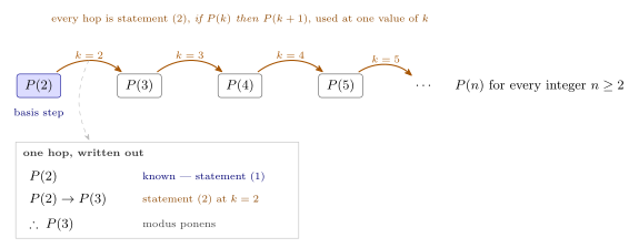
Figure 217: Why those two statements are enough. The basis step pins one statement true; every hop after it is the same general implication used at one more value of \(k\), so each conclusion becomes the next premise. The panel writes one hop out in full — it is a single modus ponens, nothing more.
Nothing here is special to 5. \(P(5)\) is reached in three hops, but the chain never stops, so \(P(n)\) is true for each integer \(n \geq 2\).
Both statements are needed. Statement 2 alone gives nothing: an implication \(P(k) \to P(k+1)\) is true in three of the four rows of its truth table — including both rows where \(P(k)\) is false. Without the basis step pinning \(P\) true somewhere, the chain has nothing to start from and every link stays vacuously true while every \(P(n)\) stays false.
The shape of an induction proof
Four steps, and it is worth naming each one explicitly in the write-up so the reader can follow the argument:
- Define the predicate. Let \(P(n)\) denote (the statement, with \(n\) free).
- Basis step. Prove the predicate is true at the smallest value of \(n\) in the claim — evaluate the two sides separately and observe they agree.
- Inductive hypothesis. Suppose \(k\) is an integer at or above the basis value, and that the predicate is true for \(n = k\). Write out what \(P(k)\) actually says.
- Inductive step. Prove \(P(k+1)\) follows, i.e. \(\forall k \in \mathbb{Z}\) with \(k \geq\) (basis), if \(P(k)\) is true then \(P(k+1)\) is true. Start from the LHS of \(P(k+1)\), use the inductive hypothesis somewhere (say where), and arrive at the RHS of \(P(k+1)\).
Then conclude: therefore, by the principle of mathematical induction, … for each integer \(n \geq\) (basis).
One thing about the order. In the write-up, the inductive step’s goal — prove that \(\forall k \in \mathbb{Z}\) with \(k \geq\) (basis), if \(P(k)\) is true then \(P(k+1)\) is true — goes on the line above the inductive hypothesis, and the assumption is made underneath it: goal first, assumption second. The numbering above counts the four actions; the goal line itself is not numbered. Write the goal down, then assume, then work.
Worked example — a summation
Prove that for each integer \(n \geq 1\), \(\displaystyle\sum_{i=1}^{n} (3i+2) = \frac{3n^2 + 7n}{2}\).
Proof. Let \(P(n)\) denote the predicate \(\displaystyle\sum_{i=1}^{n} (3i+2) = \frac{3n^2+7n}{2}\).
Basis step. Prove the predicate is true for \(n = 1\).
LHS of \(P(1)\): \(\displaystyle\sum_{i=1}^{1}(3i+2) = 3 \cdot 1 + 2 = 5\). RHS of \(P(1)\): \(\dfrac{3(1^2) + 7(1)}{2} = \dfrac{3+7}{2} = 5\). Therefore \(P(1)\) is true.
Inductive step. Prove that \(\forall k \in \mathbb{Z}\) with \(k \geq 1\), if \(P(k)\) is true then \(P(k+1)\) is true.
Inductive hypothesis: suppose \(k \geq 1\) is an integer and the predicate is true for \(n = k\) — that is, \(\displaystyle\sum_{i=1}^{k}(3i+2) = \frac{3k^2+7k}{2}\).
LHS of \(P(k+1)\):
\[\sum_{i=1}^{k+1}(3i+2) = \sum_{i=1}^{k}(3i+2) + \big(3(k+1)+2\big)\] \[= \frac{3k^2+7k}{2} + 3k + 5 \qquad \text{(by the inductive hypothesis } P(k)\text{)}\] \[= \frac{3k^2 + 13k + 10}{2} = \frac{3(k^2+2k+1) + 7k + 7}{2} = \frac{3(k+1)^2 + 7(k+1)}{2}\]
which is the RHS of \(P(k+1)\).
Therefore, by the principle of mathematical induction, \(\displaystyle\sum_{i=1}^{n}(3i+2) = \frac{3n^2+7n}{2}\) for each integer \(n \geq 1\).
The move at the first line is splitting off the last term (see sequences-and-summations) — that is what exposes the \(P(k)\) sum so the hypothesis can be applied to it. Figure 218 tracks that one expression through the chain.
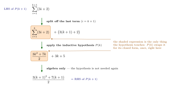
Figure 218: Where the inductive hypothesis actually enters. Splitting off the last term turns the LHS of \(P(k+1)\) into the LHS of \(P(k)\), plus one more term; the hypothesis is then spent exactly once, swapping that sum for its closed form; everything below is algebra. The shading follows that one expression from line to line.
Before starting the chain, write down what the RHS of \(P(k+1)\) actually is — here \(\frac{3(k+1)^2 + 7(k+1)}{2}\). Without it you are simplifying with no idea what counts as finished; with it, the last algebraic step is obvious, because you already know the shape you are steering the numerator into.
Induction with inequalities
Be careful when manipulating inequalities. The rules that hold:
| Given | Conclusion |
|---|---|
| \(a < b\) | \(a + x < b + x\), regardless of the sign of \(x\) |
| \(a < b\), \(x\) positive | \(ax < bx\) |
| \(a < b\), \(x\) negative | \(ax > bx\) — the direction flips |
| \(a < b\), \(x\) zero | \(ax = bx\) |
| \(a < b\) and \(x < y\) | \(a + x < b + y\) |
| \(a < b\) and \(x > y\) | nothing can be concluded about \(a + x\) |
All of these still hold with \(<\) and \(>\) replaced by \(\leq\) and \(\geq\).
Worked example — \(n^2 < 2^n\)
Prove that for each integer \(n \geq 5\), \(n^2 < 2^n\).
Proof. Let \(P(n)\) be the predicate \(n^2 < 2^n\).
Basis step. Consider \(n = 5\). Then \(n^2 = 25\) and \(2^n = 32\). Since \(25 < 32\), \(P(5)\) is true.
Inductive hypothesis. Suppose \(k \geq 5\) is an integer and \(P(k)\) is true. Thus \(k^2 < 2^k\), and hence \(2k^2 < 2 \cdot 2^k\).
Inductive step. Consider \(n = k+1\); the goal is \((k+1)^2 < 2^{k+1} = 2 \cdot 2^k\).
\[(k+1)^2 = k^2 + 2k + 1 < k^2 + 2k + k = k^2 + 3k < k^2 + k^2 = 2k^2 < 2(2^k) = 2^{k+1}\]
The first inequality uses \(1 < k\) (since \(k \geq 5\)); the second uses \(3k < k \cdot k\), which holds because \(5 \leq k\); the last uses the inductive hypothesis. Thus \(P(k+1)\) is true.
Therefore, by PMI, for each integer \(n \geq 5\), \(n^2 < 2^n\).
The pattern for an inequality is a chain: start at the LHS of \(P(k+1)\) and relax it one step at a time — each step justified by a rule from the table or by the inductive hypothesis — until it reaches the RHS of \(P(k+1)\). Every step must be an inequality in the same direction, or the chain says nothing.
The inductive step must hold at every \(k\)
Including the first one. An inductive step that is sound for all large \(k\) but fails at the basis value leaves a gap the chain cannot cross, and the induction proves nothing beyond the basis case — even though every individual line of the argument can look correct.
The classic demonstration is the ‘proof’ that all numbers are equal, whose inductive step is valid for every \(k \geq 2\) and false at \(k = 1\); it is picked apart in 2026-08-31-recursive-definitions. When checking an induction proof, run the inductive step at the smallest \(k\) it claims to cover and see whether it still says anything.
Strong induction
When the inductive step needs more than just the immediately preceding case — typically because a recurrence reaches back several terms, or because the step splits a number into two smaller ones it cannot control — ordinary induction is not enough. See strong-induction-and-the-well-ordering-principle for the stronger form, how many base cases it demands, and the well-ordering principle it is equivalent to.
See also
- sequences-and-summations · strong-induction-and-the-well-ordering-principle · proof-techniques
- solving-recurrence-relations — induction used to prove an explicit formula for a recursively defined sequence
- inclusion-exclusion — the rule for \(n\) sets, from the rule for two by splitting off the last set, an induction on \(n\)
- 2026-08-24-sequences-and-mathematical-induction — Lecture 13
- practice-problems — §17 Mathematical Induction, with full worked solutions
Modular Arithmetic, Floor & the Quotient-Remainder Theorem
Floor and ceiling
For a real number \(x\):
- \(\lfloor x \rfloor\) — the floor: move left on the number line to the nearest integer.
- \(\lceil x \rceil\) — the ceiling: move right on the number line to the nearest integer.
So \(\lfloor -3.2 \rfloor = -4\) and \(\lceil -3.2 \rceil = -3\); \(\lfloor 3.2 \rfloor = 3\) and \(\lceil 3.2 \rceil = 4\). Negative numbers are where this goes wrong most often — floor of \(-3.2\) is \(-4\), not \(-3\).
To use floor or ceiling in a proof, it is usually easiest to rewrite the expression as an integer plus an amount between 0 and 1. For instance, in proving “if \(n\) is an odd integer then \(\lceil \frac{n}{2} \rceil = \lfloor \frac{n}{2} \rfloor + 1\)”, write
\[\frac{n}{2} = \frac{2k+1}{2} = k + \frac{1}{2}\]
for some integer \(k\); then \(k + \frac{1}{2}\) sits strictly between \(k\) and \(k+1\), so the floor is \(k\) and the ceiling is \(k+1\). The same move handles things like \(\big\lfloor (p^3 + 4p^2 + 5) + \frac{1}{4} \big\rfloor\) where \(p \in \mathbb{Z}\).
Two ways to compute \(\lfloor \frac{-32}{5} \rfloor\):
- Fraction approach: \(\lfloor \frac{-32}{5} \rfloor = \lfloor \frac{-30}{5} - \frac{2}{5} \rfloor = \lfloor -6 - \frac{2}{5} \rfloor = -7\) (something smaller than \(-6\)).
- Decimal approach: \(\lfloor -6.4 \rfloor = \lfloor -6 - 0.4 \rfloor = -7\).
And \(\lceil \frac{-32}{5} \rceil = -6\).
\(\forall x \in \mathbb{R}, \lfloor x^2 \rfloor = \lfloor x \rfloor^2\) is false — take \(x = \frac{3}{2}\): \(\lfloor \frac{9}{4} \rfloor = 2\) but \(\lfloor \frac{3}{2} \rfloor^2 = 1^2 = 1\).
The quotient-remainder theorem
Given any integer \(n\) and positive integer \(d\), there exist unique integers \(q\) and \(r\) such that
\[n = dq + r \quad \text{and} \quad 0 \leq r < d\]
\(q\) is the quotient (\(n \operatorname{div} d\)) and \(r\) is the remainder (\(n \bmod d\)). Explicitly:
\[q = \left\lfloor \frac{n}{d} \right\rfloor \qquad r = n - d\left\lfloor \frac{n}{d} \right\rfloor\]
With \(d = 6\):
| \(n\) | \(n = dq + r\) | \(q\) | \(r\) |
|---|---|---|---|
| \(53\) | \(6 \cdot 8 + 5\) | \(8\) | \(5\) |
| \(20\) | \(6 \cdot 3 + 2\) | \(3\) | \(2\) |
| \(-19\) | \(6 \cdot (-4) + 5\) | \(-4\) | \(5\) |
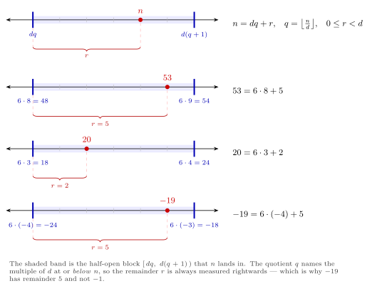
Figure 219: Why the remainder is never negative: the general case and the three \(d = 6\) examples on the number line. Each shaded band is one block \([dq, d(q+1))\) of width \(d\); the quotient names the multiple of \(d\) at or below \(n\), so \(r\) is always the rightward gap from that multiple, and \(-19\) therefore has remainder \(5\) rather than \(-1\).
Negative \(n\) is the case to watch: the remainder is still required to be non-negative, so \(-19 \bmod 6 = 5\), not \(-1\). Likewise \(-95 = 11(-9) + 4\), so \(-95 \operatorname{div} 11 = -9\) and \(-95 \bmod 11 = 4\). And \(58 = 11 \cdot 5 + 3\), so \(58 \operatorname{div} 11 = 5\), \(58 \bmod 11 = 3\).
\(\bmod\) versus \(\equiv\) — take care with notation
These are different statements.
- \(n \bmod d = r\) — an equality between numbers: the remainder when \(n\) is divided by \(d\) is \(r\), with \(0 \leq r < d\).
- \(m \equiv n \pmod{d}\) — a relation between \(m\) and \(n\): they leave the same remainder when divided by \(d\).
Example: \(5 \bmod 4 = 1\) and \(9 \bmod 4 = 1\), so \(9 \equiv 5 \pmod 4\) — but \(9 \bmod 4 \neq 5\).
Two equivalent definitions of congruence
For \(m, n, d \in \mathbb{Z}\) with \(d > 0\):
- Definition 1: \(m \equiv n \pmod d\) iff \(m\) and \(n\) have the same remainder under the quotient-remainder theorem.
- Definition 2: \(m \equiv n \pmod d\) iff \(d \mid (m - n)\).
Definition 2 is usually the faster one to check, and the one to reach for in proofs (see divisibility-and-factorisation).
Worked both ways — is \(-50 \equiv 22 \pmod 8\)?
- Definition 1: \(-50 = -56 + 6 = 8(-7) + 6\), so \(-50 \bmod 8 = 6\); and \(22 = 16 + 6\), so \(22 \bmod 8 = 6\). Same remainder, so yes.
- Definition 2: \(22 - (-50) = 72 = 8 \cdot 9\), so \(8 \mid \big(22 - (-50)\big)\), so yes.
Similarly \(53 \equiv -19 \pmod 6\) (both leave remainder 5; and \(53 - (-19) = 72\) is divisible by 6), while \(53 \not\equiv 20 \pmod 6\).
Arithmetic with congruences
Lemma: if \(a \equiv b \pmod d\) and \(m \equiv n \pmod d\), then \[a + m \equiv b + n \pmod d \qquad \text{and} \qquad am \equiv bn \pmod d\]
That is, you may substitute any number for a congruent one before adding or multiplying — which is what makes modular arithmetic cheap.
For example, \(8 \equiv 2 \pmod 3\) and \(46 \equiv 1 \pmod 3\), so \(8 \cdot 46 \equiv 2 \cdot 1 \equiv 2 \pmod 3\) and \(8 + 46 \equiv 2 + 1 \equiv 0 \pmod 3\).
Worked: suppose \(x \bmod 6 = 4\) and \(y \bmod 6 = 3\).
- \((x + y) \bmod 6\): \(x + y \equiv 4 + 3 \equiv 7 \equiv 1 \pmod 6\), so the answer is \(1\).
- \((5x^2 + 4y) \bmod 6\): \(5x^2 + 4y \equiv 5(4)^2 + 4(3) \equiv 5(16) + 12 \equiv 5(4) \equiv 20 \equiv 2 \pmod 6\) — applying the lemma at each step.
Worked: if \(m \bmod 6 = 4\), what is \(35m \bmod 6\)? Since \(35 \bmod 6 = 5\), \(35m \equiv 5 \cdot 4 \equiv 20 \equiv 2 \pmod 6\). And \(3m^2 + 2m + 1 \equiv 3(4)^2 + 2(4) + 1 \equiv 12(4) + 8 + 1 \equiv 8 + 1 \equiv 3 \pmod 6\) — \(3 \cdot 4^2\) is \(12 \cdot 4\), and that term drops out whole, since \(6 \mid 12\).
Worked: an integer \(n\) leaves remainder 4 on division by 7 — what is the remainder of \(3n\)? Write \(n = 7k + 4\); then \(3n = 21k + 12 = 7(3k + 1) + 5\), so the remainder is \(5\). (The course’s solutions PDF has this step as \(7(3k) + 5\), which is \(21k + 5\), not \(21k + 12\); the quotient is \(3k+1\). The answer of 5 is unaffected — see practice-problems.)
Worked: \(m\) leaves remainder 9 on division by 11 — what remainder does \(4m\) leave on division by 22? Write \(m = 11k + 9\); then \(4m = 44k + 36 = 22(2k+1) + 14\), so the remainder is \(14\). (Note the modulus changed, so you cannot just reduce mod 11.)
Divisibility tests
Modular arithmetic explains the familiar tests. A positive integer is divisible by 3 if and only if the sum of its digits is divisible by 3, because \(10 \equiv 1 \pmod 3\) and hence \(10^k \equiv 1 \pmod 3\) for every \(k \in \mathbb{Z}^+\) (apply the multiplication half of the lemma repeatedly: \(10^2 \equiv 1\) from \(a = m = 10\), \(b = n = 1\); then \(10^3 \equiv 1\) from \(a = 10^2\), \(m = 10\); and so on).
\[254 \equiv 2 \cdot 100 + 5 \cdot 10 + 4 \cdot 1 \equiv 2 + 5 + 4 \equiv 11 \equiv 2 \pmod 3\]
so \(254\) is not divisible by 3 and leaves remainder 2 (checking: \(254 = 3 \cdot 84 + 2\)). Whereas
\[3252 \equiv 3 + 2 + 5 + 2 \equiv 12 \equiv 0 \pmod 3\]
so \(3 \mid 3252\).
Worked proofs
For any odd integer \(n\), \(n^2 \bmod 4 = 1\).
Suppose \(n\) is odd, so \(n = 2k+1\) for some \(k \in \mathbb{Z}\). Then \[n^2 = (2k+1)^2 = 4k^2 + 4k + 1 = 4(k^2 + k) + 1.\] Since \(k^2 + k \in \mathbb{Z}\) and \(0 \leq 1 < 4\), the quotient-remainder theorem gives \(n^2 \bmod 4 = 1\). \(\square\)
Hence for any odd integer \(n\), \(\left\lfloor \frac{n^2}{4} \right\rfloor = \frac{n^2 - 1}{4}\). Two routes:
- Method 1 — expand both sides. With \(n = 2k+1\): LHS \(= \lfloor \frac{4k^2+4k+1}{4} \rfloor = \lfloor (k^2+k) + \frac{1}{4} \rfloor = k^2 + k\). RHS \(= \frac{(2k+1)^2 - 1}{4} = \frac{4k^2+4k}{4} = k^2 + k\). Equal.
- Method 2 — use \(r = n - d\lfloor \frac{n}{d} \rfloor\). With number \(n^2\), divisor \(4\), remainder \(1\): \(1 = n^2 - 4\lfloor \frac{n^2}{4} \rfloor\), so \(4\lfloor \frac{n^2}{4} \rfloor = n^2 - 1\) and \(\lfloor \frac{n^2}{4} \rfloor = \frac{n^2-1}{4}\).
For all odd integers \(n\), \(\left\lfloor \frac{n^2}{4} \right\rfloor = \left(\frac{n-1}{2}\right)\left(\frac{n+1}{2}\right)\) — true, since with \(n = 2k+1\) the right-hand side is \(\frac{2k}{2} \cdot \frac{2k+2}{2} = k(k+1)\), matching the \(k^2 + k\) above.
If \(y\) is any integer, then \(y^2\) divided by 5 leaves remainder 0, 1 or 4 — never 2 or 3.
Fix \(y \in \mathbb{Z}\). By the quotient-remainder theorem, \(y = 5m + r\) for some \(m \in \mathbb{Z}\) and \(r \in \{0,1,2,3,4\}\). Then \[y^2 = 25m^2 + 10mr + r^2 \equiv r^2 \pmod 5.\] Checking each case: \(0^2 \equiv 0\), \(1^2 \equiv 1\), \(2^2 \equiv 4\), \(3^2 \equiv 9 \equiv 4\), \(4^2 \equiv 16 \equiv 1 \pmod 5\). So \(y^2 \equiv 0, 1\) or \(4 \pmod 5\). \(\square\)
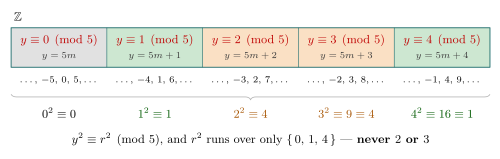
Figure 220: The case split the proof above runs on: \(\mathbb{Z}\) cut into the five residue classes mod 5. The tints group the classes by the remainder their square leaves, which is what makes \(2\) and \(3\) unreachable.
This “split into cases by remainder” move is the standard way to prove something about every integer using modular arithmetic.
See also
- divisibility-and-factorisation · gcd-lcm-and-euclidean-algorithm · proof-techniques
- sets-and-set-notation — congruence classes as sets, and the partitions of \(\mathbb{Z}\) they give
- equivalence-relations · integers-modulo-n — congruence as an equivalence relation, and its classes as the number system \(\mathbb{Z}_n\)
- pigeonhole-principle — the \(n\) remainders as pigeonholes: among any \(n + 1\) integers, two differ by a multiple of \(n\)
- practice-problems — §14 Modular Arithmetic, with full worked solutions
One-to-One and Onto Functions
The two properties a function \(f : X \to Y\) can have beyond being a function at all — injective (one-to-one) and surjective (onto) — with the proof templates for showing each and for showing its failure. Together they make a bijection, which is what inverse-functions needs. The definition of a function is in functions-on-general-sets; the lecture is 2026-09-07-functions-one-to-one-onto-inverse.
The definitions
Let \(f\) be a function, \(f : X \to Y\).
Injective function (one-to-one function): \(\forall x_1, x_2 \in X\), if \(f(x_1) = f(x_2)\) then \(x_1 = x_2\).
Surjective function (onto function): \(\forall y \in Y\), \(\exists x \in X\) such that \(f(x) = y\).
A function that is both one-to-one and onto is a bijection.
In words: one-to-one means no two inputs share an output — different inputs, different outputs. Onto means every element of the co-domain is hit — the range is the whole of \(Y\). Each name has a Latin and an English form, used interchangeably: injective / one-to-one, surjective / onto, bijective / one-to-one correspondence.
The two are about opposite ends of the arrows. One-to-one is a condition on the domain side: arrows never merge. Onto is a condition on the co-domain side: nothing is left unreached. They are independent, and all four combinations occur:
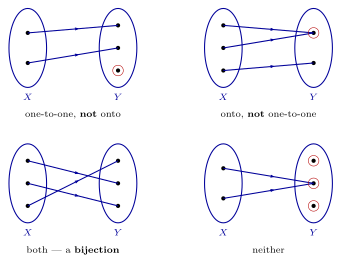
Figure 221: The four combinations, on the smallest sets that show them. Top left: one-to-one but not onto — arrows never merge, but the third dot of \(Y\) is missed. Top right: onto but not one-to-one — everything in \(Y\) is hit, but two arrows merge. Bottom left: both, a bijection — a perfect pairing. Bottom right: neither. A red ring marks the offending element of \(Y\) in each failing panel — a target that two arrows share, or a dot no arrow reaches; in the neither panel it marks one of each kind.
For finite sets the picture gives a counting fact for free: one-to-one forces \(|X| \leq |Y|\), onto forces \(|X| \geq |Y|\), and a bijection forces \(|X| = |Y|\). That is the beginning of the next topic, [cardinality], where the same three facts become the definitions of \(\leq\), \(\geq\) and \(=\) for sets of any size.
On the real line
The graph versions of the two tests:
| Test on the graph | Example | |
|---|---|---|
| one-to-one | no horizontal line meets the graph twice | \(2^x\) passes; \(x^3 - x\) fails, \(x^2\) fails |
| onto \(\mathbb{R}\) | every horizontal line meets the graph at least once | \(x^3 - x\) passes; \(2^x\) fails (never \(\leq 0\)), \(x^2\) fails |
The vertical line test decides whether a curve is a function at all (functions-on-general-sets); the horizontal line test decides one-to-one.
Changing the co-domain
Onto depends on the declared co-domain, so it can be switched on by declaring a smaller one:
\[f : \mathbb{R} \to \mathbb{R}, \; f(x) = x^2 \text{ is not onto}; \qquad g : \mathbb{R} \to \mathbb{R}^{\geq 0}, \; g(x) = x^2 \text{ is onto.}\]
Same pairs, different function, because \(Y\) is part of what a function is. Any function becomes onto its own range. One-to-one, by contrast, is a fact about the pairs alone and cannot be adjusted by relabelling the co-domain — though it can be switched on by shrinking the domain, which is how \(\sqrt{\;}\) gets to be the inverse of \(x^2\) on \(\mathbb{R}^{\geq 0}\).
How to prove it
| To show \(f : X \to Y\) is … | Template |
|---|---|
| one-to-one | Suppose \(x_1, x_2 \in X\) with \(f(x_1) = f(x_2)\). … Hence \(x_1 = x_2\). \(\square\) |
| not one-to-one | Exhibit \(x_1, x_2 \in X\) with \(x_1 \neq x_2\) and \(f(x_1) = f(x_2)\). |
| onto | Let \(y \in Y\). Take \(x = \ldots\) (in terms of \(y\)). Check \(x \in X\). Check \(f(x) = y\). \(\square\) |
| not onto | Exhibit \(y \in Y\) such that \(f(x) \neq y\) for all \(x \in X\) (and say why). |
The shape follows the quantifiers (quantified-statements). One-to-one and onto are both universal statements, so proving them means starting from an arbitrary element and arguing in general; their negations are existential, so disproving means producing one witness. This is the same logic as the element method for sets (proving-set-properties), and the same warning applies: checking examples proves neither property, it can only disprove one.
One-to-one: algebra
\(g : \mathbb{Z} \to \mathbb{Z}^{\text{odd}}\), \(g(x) = 2x + 3\).
Let \(x_1, x_2 \in \mathbb{Z}\) with \(g(x_1) = g(x_2)\). Then \(2x_1 + 3 = 2x_2 + 3\), so \(2x_1 = 2x_2\), so \(x_1 = x_2\). \(\therefore g\) is one-to-one. \(\square\)
The proof is “undo the function”: peel operations off both sides until the inputs are exposed. Every step must be reversible-in-effect — dividing by 2 is fine; squaring both sides would not be, which is exactly why \(x^2\) is not one-to-one.
Onto: solve backwards, then run forwards
Same \(g\). Scratch work (not part of the proof): want \(x\) with \(2x + 3 = y\), so \(x = \frac{y - 3}{2}\).
Proof. Let \(y \in \mathbb{Z}^{\text{odd}}\). Take \(x = \frac{y-3}{2}\). Since \(y\) is odd, \(y - 3\) is even, so \(x \in \mathbb{Z}\). And \(g(x) = 2 \cdot \frac{y-3}{2} + 3 = y\). \(\therefore g\) is onto. \(\square\)
Three moves, always in this order: name the candidate, check it is in the domain, check it maps to \(y\). The middle one is where onto proofs go wrong. Here it is the only place the oddness of \(y\) is used; drop it and the same lines “prove” that \(2x + 3\) is onto all of \(\mathbb{Z}\), which is false (\(y = 4\) needs \(x = \frac{1}{2}\)).
Pairs as inputs
\(f : \mathbb{R} \times \mathbb{R} \to \mathbb{R} \times \mathbb{R}\), \(f((x,y)) = (y + 1, 2x)\).
One-to-one. Suppose \(f((x_1,y_1)) = f((x_2,y_2))\). Then \((y_1 + 1, 2x_1) = (y_2 + 1, 2x_2)\), so \(y_1 + 1 = y_2 + 1\) and \(2x_1 = 2x_2\); hence \(y_1 = y_2\) and \(x_1 = x_2\), so \((x_1,y_1) = (x_2,y_2)\). \(\square\)
Onto. Let \((a,b) \in \mathbb{R} \times \mathbb{R}\). Take \(\left(\frac{b}{2}, a - 1\right) \in \mathbb{R} \times \mathbb{R}\). Then \(f\!\left(\left(\frac{b}{2}, a-1\right)\right) = ((a-1)+1, 2 \cdot \frac{b}{2}) = (a,b)\). \(\square\)
Two ordered pairs are equal exactly when both coordinates are, so one equation of pairs is two equations of numbers, and both must be carried through. The coordinates also cross over — the output’s first entry comes from the input’s second — which is why the candidate in the onto proof has \(b\) first.
Disproofs
\(f : \mathbb{Z} - \{-1,0,1\} \to \mathbb{Z}^{>1}\), \(f(x) =\) the largest prime divisor of \(x\).
Not one-to-one: \(f(10) = 5 = f(15)\) and \(10 \neq 15\). Not onto: \(4 \in \mathbb{Z}^{>1}\), but \(4\) is not prime, so no \(x\) has \(f(x) = 4\) — the range of \(f\) is the set of primes, a proper subset of \(\mathbb{Z}^{>1}\). Both are one line, because both are witnesses.
Is it even a function?
Before either property, the candidate has to be a function. These are examples of how that fails (functions-on-general-sets):
- \(f : \mathbb{Z}^{+} \to \mathbb{Z}^{+}\), \(f(n) = \frac{(n+1)(n+3)}{3}\) — lands outside the co-domain (\(n = 1\) gives \(\frac{8}{3}\)).
- \(f : \mathbb{Q} \to \mathbb{Z}\), \(f\!\left(\frac{m}{n}\right) = m\) — one input, two values: \(f\!\left(\frac{1}{2}\right) = 1\) but \(f\!\left(\frac{2}{4}\right) = 2\), and \(\frac{1}{2} = \frac{2}{4}\). A rule that depends on how the input is written is not well defined.
- \(\{(x,y) : y^2 = x\}\) and \(\{(x,y) : x = \lvert y \rvert\}\) — one input, two values again: \((4,2)\) and \((4,-2)\); \((1,1)\) and \((1,-1)\).
A constant function (\(f(x) = 1\)) and \(f(n) = n!\) on \(\mathbb{Z}^{+}\) are functions; the constant one is neither one-to-one nor onto \(\mathbb{R}\), which makes it the fourth panel of Figure 221.
See also
- inverse-functions — what a bijection buys you
- composition-of-functions — how the two properties behave under \(g \circ f\)
- functions-on-general-sets — the definition, co-domain versus range
- counting-selections — a one-to-one function from an \(r\)-element set to an \(n\)-element set picks \(r\) different images in order, so there are \(\frac{n!}{(n-r)!}\) of them
- pigeonhole-principle — no function from a finite set to a smaller one is one-to-one, the pigeonhole principle
- quantified-statements · proof-techniques — why the templates have the shape they have
- 2026-09-07-functions-one-to-one-onto-inverse — Lecture 19
- practice-problems — §25
Partial Order Relations
A partial order is a relation that ranks the elements of a set: it is reflexive, antisymmetric and transitive. If in addition every two elements can be compared, it is a total order. The property that is new here is in antisymmetric-relations, and the picture of a partial order is its Hasse diagram. First met in 2026-09-22-partial-order-relations.
The definitions
A relation \(R\) on a set \(S\) is a partial order relation if and only if \(R\) is
- Reflexive;
- Antisymmetric; and
- Transitive.
If \(R\) is a relation on a set \(S\), then two elements \(a, b \in S\) are comparable if and only if \(a \mathrel{R} b\) or \(b \mathrel{R} a\).
A relation \(R\) on a set \(S\) is a total order relation if and only if \(R\) is
- Reflexive;
- Antisymmetric;
- Transitive; and
- Any two elements of \(S\) are comparable.
Any total order relation is a partial order relation.
A partial order relation is a total order relation if and only if every two elements are comparable.
The model is \(\leq\) on numbers, and it helps to read \(a \mathrel{R} b\) as “\(a\) is below or equal to \(b\)”. Partial refers to condition 4 being absent. In a partial order some pairs may not be ranked against each other at all. Partial does not mean “not total”: a total order is a partial order that happens to rank every pair.
Comparable elements
Two elements are comparable when they are related in some direction. They are non-comparable when neither \(a \mathrel{R} b\) nor \(b \mathrel{R} a\) holds.
| Relation | Comparable | Non-comparable |
|---|---|---|
| \(\subseteq\) on \(\mathcal{P}(\mathbb{Z})\) | \(\{7\}\) and \(\{7,9\}\) | \(\{7\}\) and \(\{9\}\); \(\{1,2,3\}\) and \(\{1,2,4\}\) |
| divides on \(\mathbb{Z}^{+}\) | 2 and 6 | 2 and 3 |
| \(\leq\) on \(\mathbb{R}\) | every pair | none |
The first row is worked in 2026-09-22-partial-order-relations.
- Non-comparable is not “different”. \(\{7\}\) and \(\{7,9\}\) are different and comparable.
- Non-comparable is not “disjoint” or “unlike”. \(\{1,2,3\}\) and \(\{1,2,4\}\) share two elements and are still non-comparable, because neither contains the other.
- Both directions have to fail. \(6 \nmid 2\) on its own does not make 2 and 6 non-comparable, because \(2 \mid 6\).
- The elements have to be in the set. 7 and 9 are not comparable under \(\subseteq\) on \(\mathcal{P}(\mathbb{Z})\), and not non-comparable either: they are not elements of \(\mathcal{P}(\mathbb{Z})\).
In a partial order every element is comparable with itself, because the relation is reflexive. The definition of comparable applies to any relation, and in a relation that is not reflexive an element is comparable with itself only if it has a loop, as in the six-point example of 2026-09-22-partial-order-relations.
Proving a relation is a partial order
Three labelled parts, as for an equivalence relation (equivalence-relations), with the middle one changed:
| Part | Start with | Show |
|---|---|---|
| reflexive | Let \(a \in S\). | \(a \mathrel{R} a\) |
| antisymmetric | Let \(a, b \in S\) and suppose \(a \mathrel{R} b\) and \(b \mathrel{R} a\). | \(a = b\) |
| transitive | Let \(a, b, c \in S\) and suppose \(a \mathrel{R} b\) and \(b \mathrel{R} c\). | \(a \mathrel{R} c\) |
Worked: divides on \(\mathbb{Z}^{+}\)
The proof is written out in full in 2026-09-22-partial-order-relations. Unfold \(a \mid b\) as \(b = ak\) for some \(k \in \mathbb{Z}\) (divisibility-and-factorisation).
- Reflexive. \(a = a \cdot 1\), so \(a \mid a\).
- Antisymmetric. If \(b = ak\) and \(a = b\ell\) then \(b = b(\ell k)\), so \(\ell k = 1\). Both are positive, so \(\ell = k = 1\) and \(a = b\).
- Transitive. If \(b = ak\) and \(c = b\ell\) then \(c = a(k\ell)\) and \(k\ell \in \mathbb{Z}\), so \(a \mid c\).
Worked: \(\subseteq\) on a set of sets
Let \(S\) be any set of sets, for instance a power set.
- Reflexive. Every set is a subset of itself: \(X \subseteq X\).
- Antisymmetric. If \(X \subseteq Y\) and \(Y \subseteq X\) then \(X = Y\) (sets-and-set-notation).
- Transitive. If \(X \subseteq Y\) and \(Y \subseteq Z\), then every element of \(X\) is in \(Y\) and so in \(Z\): \(X \subseteq Z\).
Proper subset, \(\subset\), is not a partial order under this definition: it is not reflexive (2026-09-17-relations-reflexivity-symmetry-transitivity). The same goes for \(<\) on \(\mathbb{R}\). Both are antisymmetric and transitive, and neither has a single loop.
Total or not
Once a relation is known to be a partial order, totality is one more “for all”: for all \(a, b \in S\), \(a \mathrel{R} b\) or \(b \mathrel{R} a\).
| How | |
|---|---|
| To show it is total | Let \(a, b \in S\). Show that \(a \mathrel{R} b\) or \(b \mathrel{R} a\), usually by splitting into cases. |
| To show it is not total | Find one pair that is not comparable. |
Divides on \(\mathbb{Z}^{+}\) is not total: \(2 \nmid 3\) and \(3 \nmid 2\). One pair that cannot be compared is the whole answer. With \(\tau\) for “divides” it is written \(2 \mathrel{\not\tau} 3\) and \(3 \mathrel{\not\tau} 2\).
A total order by cases (practice-problems, Q1): for \(x \mathrel{\rho} y \leftrightarrow x^3 - 1 < y^3\) on \(\mathbb{Z}\), take two different integers \(x, y\). Then \(x^3 \neq y^3\), so either \(x^3 < y^3\), giving \(x \mathrel{\rho} y\), or \(y^3 < x^3\), giving \(y \mathrel{\rho} x\).
Whether an order is total depends on the set. Take “divides” on \(\{1, 2, 4, 8, 16\}\). There each number divides all the later ones, every two are comparable, and the order is total. On a set that contains 2 and 3 it is not.
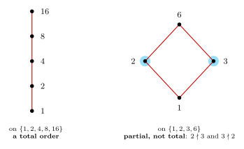
Figure 222: The relation divides on two sets, drawn as Hasse diagrams: a line means the lower number divides the upper one, and so does any path that goes up all the way. Left: on \({1,2,4,8,16}\) the diagram is a single column. Any two numbers are joined by an upward path, so every two are comparable and the order is total. Right: on \({1,2,3,6}\) the diagram branches. 2 and 3, shaded, are not joined by an upward path, since neither divides the other, so the order is partial and not total.
The examples side by side
| Relation | on | Partial order? | Total order? |
|---|---|---|---|
| \(\leq\) | \(\mathbb{R}\) | yes | yes |
| divides | \(\mathbb{Z}^{+}\) | yes | no: 2 and 3 |
| divides | \(\{1,2,4,8,16\}\) | yes | yes |
| \(\subseteq\) | \(\mathcal{P}(\{1,2,3\})\) | yes | no: \(\{1\}\) and \(\{2\}\) |
| \(\subseteq\) | \(\mathcal{P}(\mathbb{Z})\) | yes | no: \(\{7\}\) and \(\{9\}\) |
| \(x^3 - 1 < y^3\) | \(\mathbb{Z}\) | yes | yes |
| five elements in a single column | five elements | yes | yes |
| the same with a sixth element at the side | six elements | yes | no |
| \(\operatorname{weight}(s) \leq \operatorname{weight}(t)\) | binary strings of length 6 | no: not antisymmetric | — |
| \(<\) | \(\mathbb{R}\) | no: not reflexive | — |
| divides | \(\mathbb{Z}\) | no: not antisymmetric | — |
Rows 6 and 9 are Q1 and Q2 of practice-problems. Rows 7 and 8 are the two diagrams of 2026-09-22-partial-order-relations.
Equivalence relations and partial orders
The two kinds of relation the course singles out differ in one property.
| Equivalence relation | Partial order | |
|---|---|---|
| Properties | reflexive, symmetric, transitive | reflexive, antisymmetric, transitive |
| Between two different related elements | arrows both ways, always | an arrow one way only, always |
| What it does to the set | sorts it into classes | ranks it |
| Its picture | separate clusters, a partition | a Hasse diagram |
| Standard examples | \(=\), congruence mod \(n\), same parity | \(\leq\), \(\subseteq\), divides on \(\mathbb{Z}^{+}\) |
| Notes | equivalence-relations, equivalence-classes-and-partitions | partial-order-relations, hasse-diagrams |
A relation that is both an equivalence relation and a partial order is symmetric and antisymmetric, so all its arrows are loops (antisymmetric-relations), and reflexive, so it has every loop. It is equality.
Common mistakes
- Taking “partial order” to mean “not a total order”. Every total order is a partial order.
- Proving “not symmetric” where “antisymmetric” is wanted. They are different properties (antisymmetric-relations).
- Calling \(<\) or \(\subset\) a partial order. With this course’s definition a partial order is reflexive.
- Declaring a pair non-comparable after checking one direction.
- Showing a relation is total with an example. “2 and 4 are comparable” proves nothing about every pair. Not total, on the other hand, needs only one pair.
- Forgetting the set. Divides is a partial order on \(\mathbb{Z}^{+}\), a total order on \(\{1,2,4,8,16\}\), and not even antisymmetric on \(\mathbb{Z}\).
See also
- antisymmetric-relations — the property that separates a partial order from an equivalence relation
- hasse-diagrams — the standard drawing of a partial order
- reflexive-symmetric-and-transitive-relations — reflexive and transitive, with their proof templates
- equivalence-relations — the other important kind of relation
- divisibility-and-factorisation · sets-and-set-notation — the two standard partial orders, divides and \(\subseteq\)
- 2026-09-22-partial-order-relations — Lecture 25
- practice-problems — §32, with full worked solutions
The Pigeonhole Principle
If more objects are put into boxes than there are boxes, some box gets two. That is the pigeonhole principle, and it proves that something must exist (two chosen numbers that are consecutive, two subsets with the same sum, two vertices with the same degree) without finding it. This note states the principle, gives its form for functions and its generalised form, explains how to choose the pigeons and the holes, and works through the standard arguments. Counting the pigeons and the holes uses counting-principles and counting-selections. First met in 2026-10-22-pigeonhole-principle-introduction-to-graph-theory.
The principle
The pigeonhole principle. If \(n\) pigeons fly into \(m\) pigeonholes and \(n > m\), then at least one pigeonhole contains two or more pigeons.
Proof. Suppose every hole contains at most one pigeon. Then the \(m\) holes contain at most \(m\) pigeons in total. But there are \(n > m\) pigeons, a contradiction. So some hole contains at least two. \(\square\)
Three things about it:
- It says some hole has two, not which hole. A pigeonhole proof is an existence proof.
- It needs \(n > m\) strictly. Nine pigeons in nine holes can sit one per hole.
- It says nothing when \(n \le m\). Then two pigeons might share a hole or might not, and the principle gives no information either way.
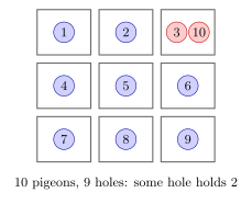
Figure 223: Ten pigeons, numbered, in nine holes. However the ten are placed, the nine holes cannot each hold at most one, since that accounts for only nine pigeons. Here pigeons 3 and 10 share the top-right hole. A different placement would make a different pair share a hole, but some hole always holds two.
As a statement about functions
Putting each pigeon in a hole is a function from the set of pigeons to the set of holes, and “two pigeons in one hole” says two inputs have the same output. So:
Pigeonhole principle, function form. If \(X\) and \(Y\) are finite sets with \(|X| > |Y|\), then no function \(f : X \to Y\) is one-to-one: there are \(x_1 \neq x_2\) in \(X\) with \(f(x_1) = f(x_2)\).
This is the first of the facts about finite sets in cardinality, and “one-to-one” is defined in one-to-one-and-onto-functions. Read this way, a pigeonhole proof has three parts: say what \(X\) is (the pigeons), say what \(Y\) is (the holes), and say what \(f\) does (which hole each pigeon goes to). Then count both sets.
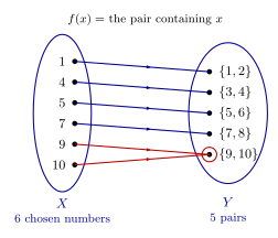
Figure 224: The function form on a small case: six numbers chosen from 1 to 10. \(X\) is the set of chosen numbers, the pigeons. \(Y\) is the set of five pairs of neighbours \({1, 2}, {3, 4}, \dots, {9, 10}\), the holes. \(f\) sends each chosen number to the pair it lies in. Since \(|X| = 6 > 5 = |Y|\), \(f\) cannot be one-to-one, so two chosen numbers, here 9 and 10, go to the same pair, and two numbers in one pair are consecutive. A different choice of six moves the collision to a different pair but cannot avoid one.
The generalised principle
Sometimes two in a hole is not enough, and the argument needs three, or more. The same proof gives the standard generalisation:
Generalised pigeonhole principle. If \(n\) pigeons fly into \(m\) pigeonholes and \(n > k \cdot m\), then at least one pigeonhole contains \(k + 1\) or more pigeons.
Proof. If every hole contained at most \(k\) pigeons, there would be at most \(k \cdot m\) pigeons, and there are more. \(\square\)
With \(k = 1\) it is the ordinary principle. An equivalent way to say it: some hole contains at least \(\lceil n/m \rceil\) pigeons, the average rounded up. If \(n > k \cdot m\) then \(n/m > k\), so \(\lceil n/m \rceil \ge k + 1\).
Example: birth months. Among any 25 people, at least 3 were born in the same month. The people are the pigeons and the 12 months are the holes. \(25 > 2 \cdot 12\), so some month has at least \(\lceil 25/12 \rceil = 3\) of them. 24 people are not enough: two born in each month have no three in the same month.
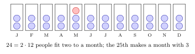
Figure 225: The generalised principle with 25 people and 12 months. Up to 24 people can be spread so that no month has more than 2, two in every month. That fills every month to its limit, so the 25th person, in red, must make some month’s count 3. In general, more than \(k \cdot m\) pigeons in \(m\) holes force some hole to hold \(k + 1\).
Choosing the pigeons and the holes
The principle is easy. The work is in choosing what the pigeons and the holes are.
- The pigeons are usually the objects the problem chooses: the numbers selected, the subsets, the people, the vertices.
- The holes must cover everything. Every pigeon has to land in some hole, and in exactly one. When the pigeons are elements of a set, the holes are a partition of that set (sets-and-set-notation).
- Two pigeons in one hole must give exactly what is wanted. This is what decides the holes. To force two consecutive numbers, make the holes pairs of consecutive numbers. To force a sum of 101, make the holes pairs that sum to 101. To force a common remainder, make the holes the remainders.
- Count both. The argument works only if there are more pigeons than holes. If the first choice of holes gives too many, look for a way to merge them, as in equal degrees, or a better bound, as in subset sums.
Many problems ask for the largest (or smallest) number with some property. The answer always has two halves:
- An example. Show that the number can be reached, by writing down a selection of that size.
- A pigeonhole argument. Show that one more forces the property to fail.
The pigeonhole half on its own proves only a bound. Without the example, the true answer might be smaller.
Worked: no two consecutive
What is the largest number of integers that can be chosen from \(\{1, 2, \dots, 100\}\) with no two consecutive?
50. The odd numbers \(1, 3, \dots, 99\) are 50 numbers with no two consecutive. For the bound, the holes are the 50 pairs \(\{1, 2\}, \{3, 4\}, \dots, \{99, 100\}\). Each pair is two consecutive numbers, so a good selection takes at most one from each pair. Choosing 51 or more puts two in some pair, and they are consecutive.
In general, from \(\{1, 2, \dots, 2m\}\) the largest selection with no two consecutive has \(m\) numbers. The holes are pairs of neighbours, \(\{2i - 1, 2i\}\).
The full question, with the wrong options, is in 2026-10-22-pigeonhole-principle-introduction-to-graph-theory.
Worked: a pair with a given sum
Prove that if 51 numbers are chosen from \(\{1, 2, \dots, 100\}\), then two of them sum to 101.
The holes are the 50 pairs \(P_i = \{i, 101 - i\}\) for \(i = 1, \dots, 50\):
\[\{1, 100\},\ \{2, 99\},\ \dots,\ \{50, 51\}.\]
Each number from 1 to 100 is in exactly one of them. 51 chosen numbers in 50 pairs put two in one pair \(P_i\), and \(i + (101 - i) = 101\).
The same holes answer any question of this shape. From \(\{1, 2, \dots, 2m\}\), any \(m + 1\) numbers include two that sum to \(2m + 1\), using the pairs \(\{i, 2m + 1 - i\}\). And \(m\) numbers are not enough: \(1, 2, \dots, m\) have no two summing to more than \(2m - 1\).
The drawing of these pairs is in 2026-10-22-pigeonhole-principle-introduction-to-graph-theory.
Worked: no three consecutive
What is the largest number of integers that can be chosen from \(\{1, 2, \dots, 60\}\) with no three consecutive?
40.
- Example. Choose everything except the multiples of 3, the numbers congruent to 1 or 2 mod 3. Any three consecutive integers include a multiple of 3, so no three chosen numbers are consecutive. That is \(60 \cdot \frac23 = 40\) numbers.
- Bound. The holes are the 20 blocks \(\{1, 2, 3\}, \{4, 5, 6\}, \dots, \{58, 59, 60\}\). A block with all three chosen is three consecutive numbers. With 41 numbers in 20 blocks, \(41 > 2 \cdot 20\), so by the generalised principle some block holds \(\lceil 41/20 \rceil = 3\) chosen numbers.
This is the generalised principle with \(k = 2\): the property needs three in one hole, not two.
Worked: two subsets with the same sum
Show that if \(A\) is any 6-element subset of \(\{1, 2, \dots, 12\}\), then \(A\) has distinct subsets \(X\) and \(Y\) with the same sum.
- Pigeons: the subsets of \(A\). There are \(2^6 = 64\) of them, including \(\emptyset\) and \(A\) (sets-and-set-notation, binomial-coefficients).
- Holes: the possible sums. Every element is positive, so a subset’s sum is between 0 (for \(\emptyset\)) and the sum of all of \(A\). Six different integers from 1 to 12 add up to at most \(7 + 8 + 9 + 10 + 11 + 12 = 57\). So there are at most 58 possible sums, \(0, 1, \dots, 57\).
- Conclusion. \(64 > 58\), so two different subsets have the same sum.
The pigeons here are not the elements of \(A\) but its subsets, which are far more numerous than the possible sums: the number of subsets doubles with each extra element, while the largest possible sum grows by at most 12. That gap is what makes the argument work. The bound on the sum has to be the tight one. Using the sum of all of \(\{1, \dots, 12\}\), 78, as the bound gives 79 holes for 64 pigeons, and the argument fails.
Leaving out \(\emptyset\) works too: 63 non-empty subsets and 57 possible sums, \(1, \dots, 57\). Either way, count the pigeons and the holes over the same collection.
The figure for \(A = \{2, 4, 6, 8, 10, 12\}\) is in 2026-10-22-pigeonhole-principle-introduction-to-graph-theory.
Worked: two with the same remainder
Show that among any \(n + 1\) integers there are two whose difference is divisible by \(n\).
The holes are the \(n\) possible remainders on division by \(n\), \(0, 1, \dots, n - 1\). Each integer has exactly one, by the quotient-remainder theorem (modular-arithmetic). \(n + 1\) integers and \(n\) remainders put two integers \(a\) and \(b\) in one hole. They have the same remainder \(r\), so \(a = nq_1 + r\) and \(b = nq_2 + r\), and \(a - b = n(q_1 - q_2)\) is divisible by \(n\).
\(n\) integers are not enough: \(0, 1, \dots, n - 1\) have all their differences between \(-(n-1)\) and \(n - 1\), and none of those but 0 is divisible by \(n\).
For example, among any 4 integers, two differ by a multiple of 3. From \(\{1, 2, \dots, 100\}\) that means 4 picks guarantee such a pair, while the 3 picks \(1, 2, 3\) do not.
Worked: two vertices of equal degree
Show that in any simple graph with at least two vertices, two vertices have the same degree.
Graphs, simple graphs and degree are in [graphs]. Said with people: in any group of two or more people, two of them have the same number of friends within the group, if friendship goes both ways.
Let the graph have \(n \ge 2\) vertices. In a simple graph a vertex is joined to at most each of the other \(n - 1\) vertices once, so every degree is one of the \(n\) values \(0, 1, \dots, n - 1\). That is \(n\) pigeons and \(n\) holes, which is not enough. The extra step is that 0 and \(n - 1\) cannot both occur. A vertex of degree \(n - 1\) is joined to every other vertex, so no vertex has degree 0. So the degrees all lie in \(\{0, 1, \dots, n - 2\}\) or all lie in \(\{1, 2, \dots, n - 1\}\). Either way there are only \(n - 1\) holes for \(n\) vertices, and two vertices share a degree.
This is the problem about five friends in 2026-07-27-welcome-and-intro-problems.
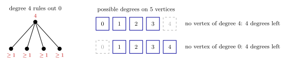
Figure 226: Why two vertices of a simple graph on 5 vertices have equal degree. The possible degrees are 0 to 4, five holes for five vertices, which forces nothing. But a vertex of degree 4 is joined to all four others, left, so each of them has degree at least 1 and none can have degree 0. So either no vertex has degree 4, top right, or none has degree 0, bottom right. In both cases only four degrees are available for five vertices, and two vertices share one.
Common mistakes
- Using it with too few pigeons. If the number of pigeons is not more than the number of holes, the principle proves nothing. It does not make the statement false either: every 5-element subset of \(\{1, \dots, 12\}\) also has two subsets with equal sums, but with 32 subsets and up to 51 possible sums the pigeonhole argument cannot show it.
- Holes that overlap. Pairs like \(\{1, 2\}, \{2, 3\}, \{3, 4\}, \dots\) share numbers, so a pigeon is in two holes and the count no longer works. The holes must split the set: every pigeon in exactly one hole.
- Holes that don’t force the property. Two pigeons in one hole must give what is wanted. Pairs \(\{1, 2\}, \{3, 4\}, \dots\) force two consecutive numbers but not two that sum to 101.
- Only half an answer. For “what is the largest”, the pigeonhole bound needs an example of that size as well, and the example needs the bound.
- Off by one in the generalised form. \(k \cdot m\) pigeons can sit \(k\) to a hole. It takes \(k \cdot m + 1\) to force \(k + 1\) in one hole: 24 people can have no three sharing a birth month, 25 cannot.
- A loose bound on the holes. Counting more holes than can actually be used (sums up to 78 rather than 57, or degrees 0 to \(n - 1\) when 0 and \(n - 1\) exclude each other) can make an argument that should work fail.
- Claiming to know which hole. The principle says some hole has two pigeons. It does not say which.
See also
- cardinality — no one-to-one function from a larger finite set to a smaller one, which is the principle for functions
- one-to-one-and-onto-functions — what one-to-one means
- [graphs] — degree, used in equal degrees
- counting-selections — counting the pigeons and the holes
- 2026-10-22-pigeonhole-principle-introduction-to-graph-theory — Lecture 33
- 2026-10-26-walks-trails-and-circuits — Lecture 34, which opens with equal degrees again
- practice-problems — §42, with full worked solutions
Practice Problems — the Semester-wide Set
This is the course’s one problem set for the whole semester — a single document rather than a per-week handout. 46 sections, one per pre-work video, each with the relevant textbook pages, a set of practice problems and full worked solutions. Everything is reproduced here in full, so you never need to open the PDF.
Applied Classes start in Week 2 and run to Week 13 — twelve of them, matching the “best 8 of 12” Applied Classes component worth 30% (see math1061). Each week’s class applies the previous week’s lecture content, so the material a class covers runs roughly one week behind the lecture column below. Which sections a given Applied Class draws on is not stated in any of the source material.
These problems belong to the roughly three hours of individual study each week, which are for revising the videos, readings and classes and completing the Practice Problems. They are the out-of-class half of the course, and they are not the same thing as the Assessed Exercises, which are done and submitted inside the class itself. (That class goes by two names, the Active Class and the Applied Class. They are one session.)
How each section is laid out
- Relevant textbook pages for Epp 4th edition and 5th (metric) edition
- Practice problems
- Solutions — full worked solutions, not just answers
- Occasionally a non-assessable Application block (see the table below)
Errata
The source document carries an errata page listing corrections made during semester. Last update: 24 August 2026, with two entries:
- On page 195, the solution to 1(b) was corrected (the note in brackets had previously copied the note from 1(a)) — already applied in §45 below.
- Question 2 in section 30 has been updated, and the original version moved to section 32 (because it refers to antisymmetry) — applied in §30 and §32 below.
If something looks wrong, post on the Ed Discussion board.
Section index
Every section is below, with its topic and textbook page ranges. Each section goes with one pre-work video (§1 with Video 001, and so on up to Video 046), and the Lecture (week) column places it in the schedule of math1061 by that video number. The Notes column links to the concept note covering that material where one exists; the rest are still ahead in the semester.
| § | Topic | Lecture (week) | 4th ed. | 5th ed. | Notes |
|---|---|---|---|---|---|
| 1 | Logical Form | L2 (wk 1) | 023–029 | 037–043 | logical-connectives |
| 2 | Logical Equivalence | L2 (wk 1) | 030–038 | 043–053 | logical-equivalence-laws |
| 3 | Conditional Statements | L3 (wk 1) | 039–050 | 053–066 | conditional-statements |
| 4 | Valid and Invalid Arguments | L4 (wk 2) | 051–063 | 066–079 | valid-argument-forms |
| 5 | Methods for Determining Validity | L5 (wk 2) | 051–063 | 066–079 | determining-argument-validity |
| 6 | Quantified Statements | L5 (wk 2) | 096–108 | 108–121 | quantified-statements |
| 7 | Negation of Quantified Statements | L6 (wk 2) | 108–117 | 122–131 | quantified-statements |
| 8 | Statements with Multiple Quantifiers | L6 (wk 2) | 117–131 | 131–146 | quantified-statements |
| 9 | Direct Proofs and Counterexamples | L7 (wk 3) | 145–163 | 160–182 | proof-techniques |
| 10 | Proof by Contradiction | L8 (wk 3) | 198–207 | 218–228 | proof-techniques |
| 11 | Proof by Contraposition | L9 (wk 3) | 198–207 | 218–228 | proof-techniques |
| 12 | Rational Numbers | L9 (wk 3) | 163–170 | 183–190 | rational-and-irrational-numbers |
| 13 | Divisibility | L10 (wk 4) | 170–179 | 190–199 | divisibility-and-factorisation |
| 14 | Modular Arithmetic | L11 (wk 4) | 482–485 | 528–531 | modular-arithmetic |
| 15 | The Euclidean Algorithm | L12 (wk 4) | 220–224 | 250–254 | gcd-lcm-and-euclidean-algorithm |
| 16 | Sequences | L13 (wk 5) | 227–244 | 258–275 | sequences-and-summations |
| 17 | Mathematical Induction | L13 (wk 5) | 244–268 | 275–301 | mathematical-induction |
| 18 | Strong Induction and the Well Ordering Principle | L14 (wk 5) | 268–279 | 301–314 | strong-induction-and-the-well-ordering-principle |
| 19 | Recursive Definitions | L15 (wk 6) | 290–304 | 325–340 | recursive-definitions |
| 20 | Solving Recurrence Relations | L16 (wk 6) | 304–328 | 340–364 | solving-recurrence-relations |
| 21 | Set Theory Definitions | L17 (wk 6) | 336–351 | 377–391 | sets-and-set-notation |
| 22 | More Definitions and Examples of Sets | L17 (wk 6) | 336–351 | 377–391 | sets-and-set-notation |
| 23 | Properties of Sets | L18 (wk 7) | 352–366 | 391–407 | proving-set-properties |
| 24 | Functions Defined on General Sets | L18 (wk 7) | 383–396 | 425–439 | functions-on-general-sets |
| 25 | one-to-one, Onto, and Inverse Functions | L19 (wk 7) | 397–416 | 439–461 | |
| 26 | Composition of Functions | L20 (wk 7) | 416–427 | 461–472 | |
| 27 | Cardinalities | L21 (wk 8) | 428–441 | 473–486 | |
| 28 | Countable and Uncountable Sets | L22 (wk 8) | 428–441 | 473–486 | |
| 29 | Relations on Sets | L23 (wk 8) | 442–449 | 487–494 | |
| 30 | Reflexivity, Symmetry, Transitivity | L23 (wk 8) | 449–459 | 495–505 | |
| 31 | Equivalence Relations | L24 (wk 9) | 459–478 | 505–523 | |
| 32 | Partial Order Relations | L25 (wk 9) | 498–515 | 546–563 | |
| 33 | Definitions and Examples of Groups | L26 (wk 9) | — | — | |
| 34 | Elementary Properties of Groups | L27 (wk 10) | — | — | |
| 35 | Group Isomorphisms | not scheduled | — | — | |
| 36 | Definitions and Examples of Fields | L28 (wk 10) | — | — | |
| 37 | Introduction to Counting | L29 (wk 11) | 516–553 | 564–604 | |
| 38 | Counting Selections | L30 (wk 11) | 516–553 | 564–604 | |
| 39 | Introduction to Probability | L31 (wk 12) | 516–553 | 564–604 | |
| 40 | Binomial Coefficients | L31 (wk 12) | 565–591 | 617–641 | |
| 41 | Inclusion Exclusion | L32 (wk 12) | 545–549 | 595–599 | |
| 42 | The Pigeonhole Principle | L33 (wk 12) | 554–565 | 604–616 | |
| 43 | Introduction to Graph Theory | L33 (wk 12) | 625–660 | 677–697 | |
| 44 | Walks, Trails and Circuits | L34 (wk 12) | 625–660 | 677–697 | |
| 45 | Matrix Representations of Graphs | L35 (wk 13) | 661–675 | 698–712 | |
| 46 | Trees | L36 (wk 13) | 683–701 | 720–742 |
§35 Group Isomorphisms has no lecture in the published schedule — the Week 10 row jumps from L27 (V34) to L28 (V36). The section itself carries no practice problems and is marked optional and will not be assessed, so the gap is deliberate.
§28 Countable and Uncountable Sets carries its own note in the source: this content will not be assessed in MATH1061. It still has a full set of problems and solutions.
Sections 33–36 (groups and fields) list no textbook page ranges.
Non-assessable application blocks
Eight sections carry an extra block of problems, not assessable for MATH1061, mostly drawn from K. Rosen, Discrete Mathematics and its Applications, 7th ed. (1991), with two from Epp. They connect the pure material to computer science, and are reproduced in full alongside their sections.
| After § | Block | Source |
|---|---|---|
| 2 | Applications to Computer Science — bit strings and logic circuits | Rosen pp. 20–24 |
| 5 | Applications of Valid and Invalid Arguments | Rosen pp. 48–68 |
| 9 | Applications of Proofs to Computer Science — resolution and automated theorem proving | Rosen pp. 74–80 |
| 15 | Trace Tables for Algorithms — the Division and Euclidean algorithms | Epp §4.8 (4th ed.) / §4.10 (5th ed.) |
| 21 | Computer Representations of Sets | Rosen pp. 134–138 |
| 28 | Computability of Functions | Rosen pp. 170–177 |
| 31 | Identifiers — C identifiers as an equivalence-relation example | Rosen pp. 608–618 |
| 37 | Runtime — counting basic instructions | Epp 5th ed. pp. 787–799 |
A note on the diagrams: the source PDF draws logic circuits, graphs and Hasse diagrams as figures. Those are reproduced here as explicit gate netlists and edge lists, which carry the same information in a form that renders everywhere.
§1 — Logical Form
Epp 4th ed. pp. 023–029 · 5th ed. (metric) pp. 037–043. Lecture 2 (week 1). Notes: logical-connectives.
Problems
Write a truth table for the statement form \(p \wedge (\sim q \vee r)\).
Suppose you know that \((\sim p \wedge q) \vee p\) is false. What can you conclude about the truth values of each of the two variables?
Let \(p\) be the statement “DATAENDFLAG is off,” \(q\) the statement “ERROR equals 0,” and \(r\) the statement “SUM is less than 1,000.” Express the following sentences in symbolic notation.
DATAENDFLAG is off, ERROR equals 0, and SUM is less than 1,000.
DATAENDFLAG is off but ERROR is not equal to 0.
DATAENDFLAG is off; however, ERROR is not 0 or SUM is greater than or equal to 1,000.
DATAENDFLAG is on and ERROR equals 0 but SUM is greater than or equal to 1,000.
Either DATAENDFLAG is on or it is the case that both ERROR equals 0 and SUM is less than 1,000.
Solutions
The truth table is
\(p\) \(q\) \(r\) \(\sim q\) \(\sim q \vee r\) \(p \wedge (\sim q \vee r)\) T T T F T T T T F F F F T F T T T T T F F T T T F T T F T F F T F F F F F F T T T F F F F T T F We know \((\sim p \wedge q) \vee p\) is false. A disjunction is false only when both parts are false, so we must have
\[p \text{ is false} \quad \text{and} \quad (\sim p \wedge q) \text{ is false.}\]
From \(p\) being false, it follows that \(\sim p\) is true. Now \((\sim p \wedge q)\) can be false only if \(q\) is false (since \(\sim p\) is already true). Hence \(q\) is false.
Therefore \(p\) is false and \(q\) is false.
\(p \wedge q \wedge r\).
\(p \wedge \sim q\).
\(p \wedge (\sim q \vee \sim r)\).
\(\sim p \wedge q \wedge \sim r\).
\(\sim p \vee (q \wedge r)\).
§2 — Logical Equivalence
Epp 4th ed. pp. 030–038 · 5th ed. (metric) pp. 043–053. Lecture 2 (week 1). Notes: logical-equivalence-laws.
Problems
Use the laws of logical equivalence to show that \(p \wedge q \equiv \; \sim (\sim p \vee \sim q)\).
Use the laws of logical equivalence to show that \(\sim (p \vee \sim q) \vee (\sim p \wedge \sim q) \equiv \; \sim p\).
For each of the following, write down a truth table for the statement, and determine whether the statement is a tautology, a contradiction, or neither.
\(((p \wedge q) \vee (q \wedge r)) \vee \sim q\)
\((\sim p \vee q) \vee (p \wedge \sim q)\)
Use De Morgan’s laws to write sentences equivalent to the following:
It is not true that I am studying Computer Science and I am studying Engineering.
I am not going to the movies this weekend or I am not going swimming this weekend.
Let \(\oplus\) denote exclusive or, which means ‘… or … but not both’. The truth table for \(p \oplus q\) is as follows:
\(p\) \(q\) \(p \oplus q\) T T F T F T F T T F F F Use a truth table to show that \((p \vee q) \wedge \sim p \equiv q \wedge \sim p\).
Use a truth table to show that \((p \oplus q) \wedge r \equiv (p \wedge r) \oplus (q \wedge r)\).
Use the laws of logical equivalence and the equivalence \(p \oplus q \equiv (p \vee q) \wedge \sim (p \wedge q)\) (which is the definition of \(\oplus\)) to show that
\[(p \oplus q) \wedge r \equiv (p \wedge r) \oplus (q \wedge r).\]
Solutions
- We have
\[\begin{aligned} \sim\big(\sim p \vee \sim q\big) &\equiv \; \sim(\sim p) \wedge \sim(\sim q) && \text{by De Morgan's law} \\ &\equiv p \wedge q && \text{by the double negative law (used twice).} \end{aligned}\]
- We have
\[\begin{aligned} \sim (p \vee \sim q) \vee (\sim p \wedge \sim q) &\equiv (\sim p \wedge \sim \sim q) \vee (\sim p \wedge \sim q) && \text{by De Morgan's law} \\ &\equiv (\sim p \wedge q) \vee (\sim p \wedge \sim q) && \text{by the double negative law} \\ &\equiv \; \sim p \wedge (q \vee \sim q) && \text{by the distributive law} \\ &\equiv \; \sim p \wedge \mathbf{t} && \text{by the negation law} \\ &\equiv \; \sim p && \text{by the identity law.} \end{aligned}\]
- We have
\(p\) \(q\) \(r\) \(p \wedge q\) \(q \wedge r\) \((p \wedge q) \vee (q \wedge r)\) \(\sim q\) \(\big((p \wedge q) \vee (q \wedge r)\big) \vee \sim q\) T T T T T T F T T T F T F T F T T F T F F F T T T F F F F F T T F T T F T T F T F T F F F F F F F F T F F F T T F F F F F F T T Thus the statement is neither a tautology nor a contradiction.
- We have
\(p\) \(q\) \(\sim p\) \(\sim p \vee q\) \(\sim q\) \(p \wedge \sim q\) \((\sim p \vee q) \vee (p \wedge \sim q)\) T T F T F F T T F F F T T T F T T T F F T F F T T T F T Hence the statement is a tautology.
- Let \(C\) be the statement “I am studying Computer Science” and \(E\) be the statement “I am studying Engineering.” The given statement is \(\sim (C \wedge E)\). By De Morgan’s law,
\[\sim (C \wedge E) \equiv (\sim C) \vee (\sim E).\]
So an equivalent statement is: “I am not studying Computer Science or I am not studying Engineering.”
- Let \(M\) be the statement “I am going to the movies this weekend” and \(S\) be the statement “I am going swimming this weekend.” The given sentence is \((\sim M) \vee (\sim S)\). By De Morgan’s law (in reverse),
\[(\sim M) \vee (\sim S) \equiv \; \sim (M \wedge S).\]
So an equivalent statement is: “It is not the case that I am both going to the movies this weekend and going swimming this weekend.”
- We have
\(p\) \(q\) \(p \vee q\) \(\sim p\) \((p \vee q) \wedge \sim p\) \(q \wedge \sim p\) T T T F F F T F T F F F F T T T T T F F F T F F Since the last two columns agree on every row, we have \((p \vee q) \wedge \sim p \equiv q \wedge \sim p\).
- We have
\(p\) \(q\) \(r\) \(p \oplus q\) \((p \oplus q) \wedge r\) \(p \wedge r\) \(q \wedge r\) \((p \wedge r) \oplus (q \wedge r)\) T T T F F T T F T T F F F F F F T F T T T T F T T F F T F F F F F T T T T F T T F T F T F F F F F F T F F F F F F F F F F F F F The columns for \((p \oplus q) \wedge r\) and \((p \wedge r) \oplus (q \wedge r)\) match on all rows, hence \((p \oplus q) \wedge r \equiv (p \wedge r) \oplus (q \wedge r)\).
- To save space, multiple laws have been applied in some steps. There are many different ways to apply the laws to prove this, so your proof may look different to this one. We have
\[\begin{aligned} &(p \wedge r) \oplus (q \wedge r) \\ &\equiv \big((p \wedge r) \vee (q \wedge r)\big) \wedge \sim \big((p \wedge r) \wedge (q \wedge r)\big) && \text{by the given equivalence (def of } \oplus) \\ &\equiv (p \vee q) \wedge r \wedge \sim \big((p \wedge r) \wedge (q \wedge r)\big) && \text{by distributive and commutative laws (for } \wedge r) \\ &\equiv (p \vee q) \wedge r \wedge \sim \big((p \wedge q) \wedge (r \wedge r)\big) && \text{by associative and commutative laws (for } \wedge) \\ &\equiv (p \vee q) \wedge r \wedge \sim \big((p \wedge q) \wedge r\big) && \text{by idempotent law} \\ &\equiv (p \vee q) \wedge r \wedge \big(\sim (p \wedge q) \vee \sim r\big) && \text{by De Morgan's law} \\ &\equiv (p \vee q) \wedge \Big(\big(r \wedge \sim (p \wedge q)\big) \vee (r \wedge \sim r)\Big) && \text{by distributive law (for } r \wedge) \\ &\equiv (p \vee q) \wedge \Big(\big(r \wedge \sim (p \wedge q)\big) \vee \mathbf{c}\Big) && \text{by negation law} \\ &\equiv (p \vee q) \wedge r \wedge \sim (p \wedge q) && \text{by identity law} \\ &\equiv (p \vee q) \wedge \sim (p \wedge q) \wedge r && \text{by associative and commutative laws (for } \wedge) \\ &\equiv (p \oplus q) \wedge r && \text{by the given equivalence (def of } \oplus) \end{aligned}\]
Application — Applications to Computer Science
Not assessable for MATH1061. Taken from K. Rosen, Discrete Mathematics and its Applications, 7th edition, 1991, pages 20–24.
Information is often represented using binary or bit strings, which are sequences consisting of zeros and ones. The length of a string is the total number of bits in it — for example \(0110110\) is a string of length 7. The logical operators \(\wedge\), \(\vee\) and \(\oplus\) extend to binary strings. The operators AND, OR and XOR are:
| \(p\) | \(q\) | \(p \vee q\) | \(p \wedge q\) | \(p \oplus q\) |
|---|---|---|---|---|
| 0 | 0 | 0 | 0 | 0 |
| 0 | 1 | 1 | 0 | 1 |
| 1 | 0 | 1 | 0 | 1 |
| 1 | 1 | 1 | 1 | 0 |
Propositional logic also applies to the design of computer hardware. A digital logic circuit receives input signals (either 0, the wire being off, or 1, on) and produces output signals which are also bits. Complicated digital logic circuits can be constructed from three basic gates: the OR gate, the NOT gate and the AND gate.
A combinational circuit uses these gates and obeys the following rules.
- Two input wires cannot be combined without a gate.
- A single input wire can be split partway and directed into two separate gates.
- An output wire from a gate can be used as input for another gate.
- No output wire from a gate can eventually feed back into that gate.
For example, the logical expression \((p \wedge \sim q) \vee \sim r\) has the combinational circuit
- \(\text{NOT}(q) \to n_1\)
- \(\text{AND}(p,\, n_1) \to a_1\)
- \(\text{NOT}(r) \to n_2\)
- \(\text{OR}(a_1,\, n_2) \to\) output \((p \wedge \sim q) \vee \sim r\)
Application problems
Find the bitwise OR, bitwise AND and bitwise XOR of each of these pairs of binary strings.
\(1011110\), \(0100001\)
\(11110000\), \(10101010\)
Construct a combinational circuit using the NOT, OR and AND gates that produces the outputs:
\((\sim p \vee \sim r) \wedge q\)
\((p \wedge \sim r) \vee (\sim q \wedge r)\)
Find the output of the following combinational circuit, simplify the expression using logical laws and construct a new circuit for the simplified expression. The circuit is
- \(\text{NOT}(p) \to n_1\)
- \(\text{NOT}(q) \to n_2\)
- \(\text{OR}(p,\, n_2) \to o_1\)
- \(\text{OR}(n_1,\, n_2) \to o_2\)
- \(\text{AND}(o_1,\, o_2) \to a_1\)
- \(\text{OR}(a_1,\, r) \to\) output
(both \(p\) and \(q\) have their wires split, feeding two gates each).
The logical binary operation NAND, denoted \(\mid\), is defined by
\[p \mid q \equiv \; \sim (p \wedge q).\]
Write down the truth table for \(\sim (p \mid q)\). Show all working.
Prove, using truth tables or otherwise, that \((p \mid p) \equiv (\sim p)\). Show all working.
Prove, using truth tables or otherwise, that \(((p \mid p) \mid (q \mid q)) \equiv p \vee q\). Show all working.
Application solutions
\[1011110 \text{ OR } 0100001 = 1111111,\] \[1011110 \text{ AND } 0100001 = 0000000,\] \[1011110 \text{ XOR } 0100001 = 1111111.\]
\[11110000 \text{ OR } 10101010 = 11111010,\] \[11110000 \text{ AND } 10101010 = 10100000,\] \[11110000 \text{ XOR } 10101010 = 01011010.\]
- The circuit is
- \(\text{NOT}(p) \to n_1\)
- \(\text{NOT}(r) \to n_2\)
- \(\text{OR}(n_1,\, n_2) \to o_1\)
- \(\text{AND}(o_1,\, q) \to\) output \((\sim p \vee \sim r) \wedge q\)
- The circuit is
- \(\text{NOT}(r) \to n_1\)
- \(\text{AND}(p,\, n_1) \to a_1\)
- \(\text{NOT}(q) \to n_2\)
- \(\text{AND}(n_2,\, r) \to a_2\)
- \(\text{OR}(a_1,\, a_2) \to\) output \((p \wedge \sim r) \vee (\sim q \wedge r)\)
The given digital logic circuit has output \(\big((p \vee \sim q) \wedge (\sim p \vee \sim q)\big) \vee r\). Using laws of logical equivalence we have
\[\begin{aligned} \big((p \vee \sim q) \wedge (\sim p \vee \sim q)\big) \vee r &\equiv \big(\sim q \vee (p \wedge \sim p)\big) \vee r && \text{by distributive and commutative laws} \\ &\equiv (\sim q \vee \mathbf{c}) \vee r && \text{by negation law} \\ &\equiv \; \sim q \vee r && \text{by identity law} \end{aligned}\]
The simplification is \(\sim q \vee r\). The simplified logic circuit is
- \(\text{NOT}(q) \to n_1\)
- \(\text{OR}(r,\, n_1) \to\) output \(\sim q \vee r\)
- We have
\(p\) \(q\) \(p \wedge q\) \(p \mid q\) \(\sim (p \mid q)\) T T T F T T F F T F F T F T F F F F T F Hence \(\sim (p \mid q)\) has the same truth values as \(p \wedge q\) (it is true exactly when both \(p\) and \(q\) are true).
- Since \(p \mid p \equiv \; \sim (p \wedge p)\), we have
\[p \mid p \equiv \; \sim (p \wedge p) \equiv \; \sim p\]
because \(p \wedge p \equiv p\) (idempotent law). Alternatively, by truth table:
\(p\) \(p \wedge p\) \(p \mid p\) \(\sim p\) T T F F F F T T The last two columns agree, so \(p \mid p \equiv \; \sim p\).
- First note from part (b) that \(p \mid p \equiv \; \sim p\) and \(q \mid q \equiv \; \sim q\). Therefore
\[\begin{aligned} (p \mid p) \mid (q \mid q) &\equiv (\sim p) \mid (\sim q) && \text{by part (b)} \\ &\equiv \; \sim\big((\sim p) \wedge (\sim q)\big) && \text{by def of NAND} \\ &\equiv p \vee q && \text{by De Morgan's law.} \end{aligned}\]
Alternatively, by truth table:
\(p\) \(q\) \(p \mid p\) \(q \mid q\) \((p \mid p) \mid (q \mid q)\) \(p \vee q\) T T F F T T T F F T T T F T T F T T F F T T F F The last two columns match, hence \((p \mid p) \mid (q \mid q) \equiv p \vee q\).
§3 — Conditional Statements
Epp 4th ed. pp. 039–050 · 5th ed. (metric) pp. 053–066. Lecture 3 (week 1). Notes: conditional-statements.
Problems
Let \(p\), \(q\) and \(r\) be statements. Use the laws of logical equivalence to show that
\[p \to (q \vee r) \equiv (p \wedge \sim q) \to r.\]
Let \(p\) and \(q\) be statement variables. Are the following statements logically equivalent? Justify your answer.
- Statement A: \((p \to q) \wedge \sim q\)
- Statement B: \(\sim (p \wedge q)\)
Write each of the following statements in the form ‘if … then …’.
A sufficient condition for the warranty to be good is that you bought the computer less than a year ago.
Jane gets seasick whenever she is on a boat.
For each of the following, write down a truth table for the statement, and determine whether the statement is a tautology, a contradiction, or neither.
\((\sim p \wedge (p \to q)) \to \sim q\)
\((p \to (q \vee r)) \leftrightarrow ((p \wedge \sim q) \to r)\)
Negate the following two statements.
If it rains, then Sue takes her umbrella.
The cakes burn if the oven temperature is too high.
Recall “a sufficient condition for \(s\) is \(r\)” means \(r\) is a sufficient condition for \(s\), and that “a necessary condition for \(s\) is \(r\)” means \(r\) is a necessary condition for \(s\). Rewrite the following statements in ‘if … then …’ form:
A sufficient condition for John’s team to win the championship is that it wins the rest of its games.
A necessary condition for this computer program to be correct is that it not produce error messages during translation.
Solutions
We have
\[\begin{aligned} p \to (q \vee r) &\equiv \; \sim p \vee (q \vee r) && \text{by definition of implication} \\ &\equiv (\sim p \vee q) \vee r && \text{by the associative law} \\ &\equiv \; \sim (p \wedge \sim q) \vee r && \text{by De Morgan's law and double negative law} \\ &\equiv (p \wedge \sim q) \to r && \text{by definition of implication.} \end{aligned}\]
Let \(A\) be the statement \((p \to q) \wedge \sim q\) and let \(B\) be the statement \(\sim (p \wedge q)\). Then
\[\begin{aligned} A &\equiv (\sim p \vee q) \wedge \sim q && \text{by definition of implication} \\ &\equiv (\sim p \wedge \sim q) \vee (q \wedge \sim q) && \text{by distributive and commutative laws} \\ &\equiv (\sim p \wedge \sim q) \vee \mathbf{c} && \text{by negation law} \\ &\equiv \; \sim p \wedge \sim q && \text{by identity law,} \end{aligned}\]
while
\[B \equiv \; \sim (p \wedge q) \equiv \; \sim p \vee \sim q \qquad \text{by De Morgan's law.}\]
Thus Statement A and Statement B are not logically equivalent because, for example, if \(p\) is false and \(q\) is true, then \(A\) is false and \(B\) is true. Hence \(A \not\equiv B\).
If you bought the computer less than a year ago, then the warranty is good.
If Jane is on a boat, then Jane gets seasick.
- Solution Option 1. The truth table for the statement is
\(p\) \(q\) \(\sim p\) \(p \to q\) \(\sim p \wedge (p \to q)\) \(\sim q\) \((\sim p \wedge (p \to q)) \to \sim q\) T T F T F F T T F F F F T T F T T T T F F F F T T T T T The statement is neither a tautology nor a contradiction.
Solution Option 2. The same truth table, written under the parts of the statement:
\(p\) \(q\) \(\sim p\) \(\wedge\) \((p \to q)\) \(\to\) \(\sim q\) T T F F T T F T F F F F T T F T T T T F F F F T T T T T order ① ④ ② ⑤ ③ The small numbers show the order in which the columns were completed. Column ④ comes from comparing columns ① and ②. Column ⑤ comes from comparing columns ③ and ④, and shows the truth values for the entire statement. This shows that this statement is neither a tautology nor a contradiction. (You don’t have to number the columns — this is just to help your understanding!)
- Solution Option 1. The truth tables for the LHS and RHS are:
\(p\) \(q\) \(r\) \(q \vee r\) \(p \to (q \vee r)\) \(\sim q\) \(p \wedge \sim q\) \((p \wedge \sim q) \to r\) T T T T T F F T T T F T T F F T T F T T T T T T T F F F F T T F F T T T T F F T F T F T T F F T F F T T T T F T F F F F T T F T Therefore the truth table for the statement is:
\(p\) \(q\) \(r\) \(\big(p \to (q \vee r)\big) \leftrightarrow \big((p \wedge \sim q) \to r\big)\) T T T T T T F T T F T T T F F T F T T T F T F T F F T T F F F T The statement is a tautology.
Solution Option 2. Another way to represent the truth table for \((p \to (q \vee r)) \leftrightarrow ((p \wedge \sim q) \to r)\):
\(p\) \(q\) \(r\) \(p \to\) \((q \vee r)\) \(\leftrightarrow\) \((p \wedge \sim q)\) \(\to r\) T T T T T T F T T T F T T T F T T F T T T T T T T F F F F T T F F T T T T T F T F T F T T T F T F F T T T T F T F F F T F T F T order ② ① ⑤ ③ ④ Here column ⑤ comes from comparing columns ② and ④. We see (from column ⑤) that this is a tautology.
- Let \(R\) be the statement “it rains” and \(U\) be the statement “Sue takes her umbrella.” The given statement is \(R \to U\). Its negation is
\[R \wedge \sim U,\]
i.e. “It rains and Sue does not take her umbrella.”
- Let \(H\) be the statement “the oven temperature is too high” and \(B\) be the statement “the cakes burn.” The given statement is \(H \to B\). Its negation is
\[H \wedge \sim B,\]
i.e. “The oven temperature is too high and the cakes do not burn.”
If John’s team wins the rest of its games, then John’s team will win the championship.
If this computer program is correct, then it does not produce error messages during translation.
§4 — Valid and Invalid Arguments
Epp 4th ed. pp. 051–063 · 5th ed. (metric) pp. 066–079. Lecture 4 (week 2). Notes: valid-argument-forms.
Problems
State truth values for the statement variables \(p\) and \(q\) that demonstrate that the following argument is invalid, and justify your answer.
Premise 1: \(q\) Premise 2: \(p \to q\) Conclusion: \(p\)
Find values of the statement variables \(a\), \(b\) and \(c\) that show that the following argument is invalid.
- \(a \to b\)
- \(\sim a \to c\)
- \(\sim b \to c\) \(\therefore\ b\)
Use a truth table to show that the following argument forms are valid.
- Elimination:
- \(p \vee q\)
- \(\sim q\) \(\therefore\ p\)
- Generalisation:
- \(p\) \(\therefore\ p \vee q\)
Use a truth table to show that the following argument is invalid.
- \((p \wedge q) \to \sim r\)
- \(p \vee \sim q\)
- \(\sim q \to p\) \(\therefore\ \sim r\)
Solutions
To show the argument is invalid, we must find truth values for \(p\) and \(q\) such that the premises are true and the conclusion is false.
Suppose \(p\) is false and \(q\) is true. Then Premise 1 (\(q\)) is true and Premise 2 (\(p \to q\)) is true (by definition of implication). However, the conclusion (\(p\)) is false. Therefore the argument is invalid.
To show the argument is invalid, we must find truth values for \(a\), \(b\) and \(c\) such that the premises are true and the conclusion is false.
Let \(a\) be false, \(b\) be false, and \(c\) be true. By definition of implication, all three premises are true, but the conclusion (\(b\)) is false, so the argument is invalid.
\(p\) \(q\) premise 1: \(p \vee q\) premise 2: \(\sim q\) conclusion: \(p\) T T T F T T F T T T F T T F F F F F T F There is only one row of the truth table in which all premises are true (the second row), and here the conclusion is true. Thus, whenever all the premises are true, the conclusion is true, so the argument is valid.
\(p\) \(q\) premise 1: \(p\) conclusion: \(p \vee q\) T T T T T F T T F T F T F F F F There are two rows for which all premises (here just the one premise) are true — the first two rows — and for each of these rows the conclusion is true. Thus, whenever all the premises are true, the conclusion is true, so the argument is valid.
We compute the truth table:
\(p\) \(q\) \(r\) \((p \wedge q) \to \sim r\) \(p \vee \sim q\) \(\sim q \to p\) Prem. 1 \(\wedge\) Prem. 2 \(\wedge\) Prem. 3 \(\sim r\) T T T F T T F F T T F T T T T T T F T T T T T F T F F T T T T T F T T T F T F F F T F T F T F T F F T T T F F F F F F T T F F T There are three rows for which all the premises are true, however for one of these rows the conclusion is false. In particular, taking \(p\) to be true, \(q\) to be false, and \(r\) to be true makes all the premises true but the conclusion false, so the argument is invalid.
§5 — Methods for Determining Validity
Epp 4th ed. pp. 051–063 · 5th ed. (metric) pp. 066–079. Lecture 5 (week 2). Notes: determining-argument-validity.
Problems
Determine whether the following arguments are valid. If the argument is valid, prove it using rules of inference. If the argument is invalid, demonstrate it with a choice of truth values for the variables.
\(p \to q\) \(q \to p\) \(\therefore\ p \vee q\)
\(p\) \(p \to q\) \(\sim q \vee r\) \(\therefore\ r\)
\(p \vee q\) \(p \to \sim q\) \(p \to r\) \(\therefore\ r\)
Write the following argument in symbolic form. Then determine whether the argument is valid or not.
An error message is received if the output is flagged. The system is running normally only if the output is not flagged. An error message is received. Therefore, the system is not running normally.
Please use the following variables:
\(p\) the output is flagged \(q\) an error message is received \(r\) the system is running normally Give truth values for the variables \(p\), \(q\), \(r\), \(s\) and \(w\) which demonstrate that the following argument is invalid.
\[\big[(p \vee q) \wedge (q \to r) \wedge ((p \wedge s) \to w) \wedge (\sim r) \wedge (q \to s)\big] \to w\]
Solutions
- The argument is invalid. When \(p\) and \(q\) are both false, all the premises are true, but the conclusion is false. One could arrive at this example by computing the following truth table:
\(p\) \(q\) \(p \to q\) \(q \to p\) \(p \vee q\) T T T T T T F F T T F T T F T F F T T F (In the last row, the premises are true, but the conclusion is false.)
- The argument is valid, and we prove this with rules of inference:
1. \(p\) Premise 2. \(p \to q\) Premise 3. \(\sim q \vee r\) Premise 4. \(q\) from 1 and 2 by Modus Ponens 5. \(r\) from 3 and 4 by elimination (and the double negative law) Therefore the argument is valid.
- Suppose the argument is invalid. Then it is possible to find truth values for the statement variables that make all the premises true and the conclusion false. For the conclusion to be false, we have \(r\) is false. Since \(r\) is false but the third premise (\(p \to r\)) is true, we must have \(p\) is false. Since \(p\) is false, this means the second premise (\(p \to \sim q\)) is also true. Now since \(p\) is false but the first premise (\(p \vee q\)) is true, we must have \(q\) is true.
Thus, with these truth values for the three variables, we have that all the premises are true, but the conclusion is false. So the argument is invalid.
The argument has the symbolic form:
1. \(p \to q\) (An error message is received if the output is flagged.) 2. \(r \to \sim p\) (The system is running normally only if the output is not flagged.) 3. \(q\) (An error message is received.) \(\therefore\) \(\sim r\) (The system is not running normally.) Suppose the argument is invalid. Then it is possible to find truth values for the statement variables that make all the premises true and the conclusion false. For the conclusion to be false, we have \(r\) is true. Since \(r\) is true, and premise 2 is true, we must have \(\sim p\) true, that is \(p\) is false. Since premise 3 is true, we have \(q\) is true.
Thus, with these truth values for the three variables, we have that all the premises are true, but the conclusion is false. So the argument is invalid.
The argument being valid is the same as this overall implication statement being a tautology.
\[\big[(p \vee q) \wedge (q \to r) \wedge ((p \wedge s) \to w) \wedge (\sim r) \wedge (q \to s)\big] \to w\]
We can write the argument as follows:
- \(p \vee q\)
- \(q \to r\)
- \((p \wedge s) \to w\)
- \(\sim r\)
- \(q \to s\) \(\therefore\ w\)
Suppose the argument is invalid. Then it is possible to find truth values for the statement variables that make all the premises true and the conclusion false. For the conclusion to be false, we have \(w\) is false. Since premise 4 is true we have \(r\) is false. Since premise 2 is true and \(r\) is false, we must have \(q\) is false. Since premise 1 is true and \(q\) is false we have \(p\) is true. Since premise 3 is true and \(w\) is false, we must have \((p \wedge s)\) false, and since \(p\) is true, this means \(s\) is false. These truth values also mean premise 5 is true.
Thus with these truth values for the variables, we have that all the premises are true, but the conclusion is false. So the argument is invalid.
Application — Applications of Valid and Invalid Arguments
Not assessable for MATH1061. Taken from K. Rosen, Discrete Mathematics and its Applications, 7th edition, 1991, pages 48–68.
Application problems
Translating English sentences into logical expressions is an essential part of specifying both hardware and software systems. Software engineers must take requirements in English and produce precise, unambiguous specifications that can be used as the basis for system development.
Consider the following predicates and domains:
Predicates:
\(F(x, y)\) disk \(x\) has more than \(y\) kilobytes of free space. \(S(m)\) mail message \(m\) can be saved. \(A(x)\) alert \(x\) is active. \(Q(m)\) message \(m\) is queued. \(T(m)\) message \(m\) is transmitted. \(D(s)\) the diagnostic monitor tracks the status of system \(s\). Domains:
\(M\) the nonempty set of all messages. \(X\) the set of all disks. \(Y\) the set of all alerts. \(S\) the set of all systems. Express the system specifications below using quantifiers and logical connectives:
At least one mail message, among the nonempty set of messages, can be saved if there is a disk with more than 10 kilobytes of free space.
Whenever there is an active alert, all queued messages are transmitted.
The diagnostic monitor tracks the status of all systems except the main console.
System specifications should be consistent; that is, they should not contain conflicting requirements that could be used to derive a contradiction. When specifications are not consistent, there would be no way to develop a system that satisfies all specifications. Logically, a system is consistent if it is possible for all the premises to be simultaneously true.
Use logical expressions and methods of logical deduction to determine whether the following specifications are consistent.
The system is in multiuser state if and only if it is operating normally. If the system is operating normally, the kernel is functioning. The kernel is not functioning or the system is in interrupt mode. If the system is not in multiuser state, then it is in interrupt mode. The system is not in interrupt mode.
The router can send packets to the edge system only if it supports the new address space. For the router to support the new address space it is necessary that the latest software release be installed. The router can send packets to the edge system if the latest software release is installed. The router does not support the new address space.
Application solutions
\((\exists x \in X \text{ s.t. } F(x, 10)) \to (\exists m \in M \text{ s.t. } S(m))\).
\((\exists y \in Y \text{ s.t. } A(y)) \to (\forall m \in M,\ (Q(m) \to T(m)))\).
Let \(c \in S\) denote the main console. \(\forall s \in S,\ (s \neq c \to D(s))\).
- Define the following variables:
\(m\) the system is in multiuser state \(n\) the system is operating normally \(k\) the kernel is functioning \(i\) the system is in interrupt mode Now we can express the specifications as follows:
- \(m \leftrightarrow n\)
- \(n \to k\)
- \(\sim k \vee i\)
- \(\sim m \to i\)
- \(\sim i\)
Solution Option 1. If these specifications are consistent, then we must be able to find truth values for each of the variables that makes all of the specifications true. Assume the specifications are consistent (so we assume each specification is true). For specification 5 to be true we know \(i\) is false. For specification 4 to be true, with \(i\) false, we know \(\sim m\) is false so \(m\) is true. For premise 1 to be true, with \(m\) true, we have \(n\) is true. For specification 2 to be true, and since \(n\) is true, we have \(k\) is true. However, now \(\sim k\) is false and \(i\) is false, which means specification 3 is false. This contradicts our assumption that all the specifications are true, and so it is impossible for the system to be consistent. Therefore, the system is not consistent.
Solution Option 2. Suppose the specifications are all true. Using laws of inference, we have
1. \(m \leftrightarrow n\) specification 2. \(n \to k\) specification 3. \(\sim k \vee i\) specification 4. \(\sim m \to i\) specification 5. \(\sim i\) specification 6. \(\sim k\) from 3 and 5 by elimination (and double negative law) 7. \(\sim n\) from 2 and 6 by Modus Tollens 8. \((m \to n) \wedge (n \to m)\) from 1 by definition of \(\leftrightarrow\) 9. \(m \to n\) from 8 by specialisation 10. \(\sim m\) from 9 and 7 by Modus Tollens 11. \(i\) from 4 and 10 by Modus Ponens But now we have both \(i\) and \(\sim i\) being true, which is a contradiction. This contradicts our assumption that all the specifications are true, and so it is impossible for the system to be consistent. Therefore, the system is not consistent.
- Define the following variables:
\(r\) the router can send packets to the edge system \(a\) the router supports the new address space \(s\) the latest software release is installed Now we can express the specifications as follows:
- \(r \to a\)
- \(a \to s\)
- \(s \to r\)
- \(\sim a\)
Assume the specifications are consistent, so each specification is true. For specification 4 to be true, \(\sim a\) is true, so \(a\) is false. For specification 1 to be true with \(a\) false we must have \(r\) is false. Now, since \(r\) is false and specification 3 is true, we have \(s\) is false. We double-check that specification 2 is true, which it is because \(a\) is false. Thus, we have found truth values of the statement variables that make all of the specifications true, so the system is consistent.
§6 — Quantified Statements
Epp 4th ed. pp. 096–108 · 5th ed. (metric) pp. 108–121. Lecture 5 (week 2). Notes: quantified-statements.
Problems
Rewrite each of the following in the form “\(\forall \underline{\phantom{xx}},\ \underline{\phantom{xx}}\).” Here, let \(D\) be the set of all dinosaurs, and let \(L\) be the set of all logicians.
All dinosaurs are extinct.
Every real number is positive, negative, or zero.
No irrational numbers are integers.
No logicians are lazy.
The number \(2{,}147{,}581{,}953\) is not equal to the square of any integer.
The number \(-1\) is not equal to the square of any real number.
Rewrite each of the following in the form “\(\exists \underline{\phantom{xx}}\) such that \(\underline{\phantom{xx}}\).” Here, let \(X\) be the set of all exercises.
Some exercises have answers.
Some real numbers are rational.
Determine whether the following statements are true or false. Justify your reasoning.
\(\forall x \in \mathbb{R},\ x \geq \frac{1}{x}\).
\(\forall a \in \mathbb{Z},\ \frac{a-1}{a} \notin \mathbb{Z}\).
\(\forall m, n \in \mathbb{Z}^+,\ mn \geq m + n\).
Solutions
\(\forall x \in D,\ x\) is extinct.
\(\forall x \in \mathbb{R},\ (x > 0 \vee x < 0 \vee x = 0)\).
\(\forall x \in \mathbb{R},\ (x \text{ is irrational} \to x \notin \mathbb{Z})\).
\(\forall x \in L,\ x\) is not lazy.
\(\forall x \in \mathbb{Z},\ x^2 \neq 2147581953\).
\(\forall x \in \mathbb{R},\ -1 \neq x^2\).
\(\exists x \in X\) such that \(x\) has an answer.
\(\exists x \in \mathbb{R}\) such that \(x \in \mathbb{Q}\).
False. Counterexample: take \(x = \frac{1}{2}\). Then \(x = \frac{1}{2}\) but \(\frac{1}{x} = 2\), so \(x \geq \frac{1}{x}\) is false.
False. Counterexample: take \(a = 1\). Then \(\frac{a-1}{a} = \frac{0}{1} = 0 \in \mathbb{Z}\).
False. Counterexample: take \(n = m = 1\). Then \(mn = 1\) but \(m + n = 2\).
§7 — Negation of Quantified Statements
Epp 4th ed. pp. 108–117 · 5th ed. (metric) pp. 122–131. Lecture 6 (week 2). Notes: quantified-statements.
Problems
Write the negation of each of the following statements, and then determine whether the original or the negation is true:
\(\forall x \in \mathbb{R}\), if \(x^2 > 9\) then \(x \geq 2\).
\(\forall n \in \mathbb{Z}^+\), \(n\) is either prime or composite.
\(\exists x, y \in \mathbb{R}\) such that \(x \notin \mathbb{Z}\) and \(y \notin \mathbb{Z}\) but \(xy \in \mathbb{Z}\).
Write down the negation of each of the following statements:
All fire engines are red.
Some apples are ripe.
A triangle with equal sides exists.
Solutions
- Original: \(\forall x \in \mathbb{R}\), if \(x^2 > 9\) then \(x \geq 2\). Negation: \(\exists x \in \mathbb{R}\) such that \(x^2 > 9\) and \(x < 2\).
The original statement is false. For instance, take \(x = -4\). Then \(x^2 > 9\) but \(x \not\geq 2\).
- Original: \(\forall n \in \mathbb{Z}^+\), \(n\) is either prime or composite. Negation: \(\exists n \in \mathbb{Z}^+\) such that \(n\) is neither prime nor composite.
The original statement is false. For instance, consider \(n = 1\), which is neither prime nor composite.
- Original: \(\exists x, y \in \mathbb{R}\) such that \(x \notin \mathbb{Z}\) and \(y \notin \mathbb{Z}\) but \(xy \in \mathbb{Z}\). Negation: \(\forall x, y \in \mathbb{R}\), if \(x \notin \mathbb{Z}\) and \(y \notin \mathbb{Z}\) then \(xy \notin \mathbb{Z}\).
The original statement is true. For instance, take \(x = \sqrt{2}\) and \(y = \sqrt{2}\). Then \(x \notin \mathbb{Z}\) and \(y \notin \mathbb{Z}\), but \(xy = 2 \in \mathbb{Z}\).
Original: All fire engines are red. Negation: There exists a fire engine which is not red.
Original: Some apples are ripe. Negation: All apples are not ripe.
Original: A triangle with equal sides exists. Negation: There does not exist a triangle with equal sides.
§8 — Statements with Multiple Quantifiers
Epp 4th ed. pp. 117–131 · 5th ed. (metric) pp. 131–146. Lecture 6 (week 2). Notes: quantified-statements.
Problems
Write down the negation of each of the following statements. Then determine whether the statement is true, or whether its negation is true.
\(\forall x, y \in \mathbb{Z}\), \(\exists z \in \mathbb{Z}\) such that \(z = x - y\).
\(\forall x \in \mathbb{R}\), \(\exists y \in \mathbb{R}\) such that \(x^2 - xy - 2y^2 = 0\).
\(\exists x \in \mathbb{Z}^+\) such that \(\forall y \in \mathbb{Z}^+\), \(x \geq y\).
\(\forall r, s \in \mathbb{R}\), if \(rs \in \mathbb{Q}\), then \(r \in \mathbb{Q}\) and \(s \in \mathbb{Q}\).
For each of the following English sentences:
For any rational number \(x\) and any negative integer \(y\) there exists a real number that is greater than the product of \(x\) and \(y\).
For every real number \(x\), there is a real number \(y\) for which \(3y = x\).
do the following:
Write the statement in symbolic form.
Write the negation of the statement in symbolic form.
Determine which of the statement or its negation is true.
Solutions
- Original: \(\forall x, y \in \mathbb{Z}\), \(\exists z \in \mathbb{Z}\) such that \(z = x - y\). Negation: \(\exists x \in \mathbb{Z}\ \exists y \in \mathbb{Z}\) such that \(\forall z \in \mathbb{Z}\), \(z \neq x - y\).
The original statement is true (and the negation is false). For any given \(x, y \in \mathbb{Z}\), choose \(z = x - y \in \mathbb{Z}\).
- Original: \(\forall x \in \mathbb{R}\), \(\exists y \in \mathbb{R}\) such that \(x^2 - xy - 2y^2 = 0\). Negation: \(\exists x \in \mathbb{R}\) s.t. \(\forall y \in \mathbb{R}\), \(x^2 - xy - 2y^2 \neq 0\).
The original statement is true (and the negation is false). For any \(x \in \mathbb{R}\), taking \(y = \frac{x}{2}\) gives
\[x^2 - x\left(\frac{x}{2}\right) - 2\left(\frac{x}{2}\right)^2 = x^2 - \frac{x^2}{2} - 2 \cdot \frac{x^2}{4} = x^2 - \frac{x^2}{2} - \frac{x^2}{2} = 0.\]
- Original: \(\exists x \in \mathbb{Z}^+\) such that \(\forall y \in \mathbb{Z}^+\), \(x \geq y\). Negation: \(\forall x \in \mathbb{Z}^+\ \exists y \in \mathbb{Z}^+\) such that \(x < y\).
The negation is true (and the original is false). For any \(x \in \mathbb{Z}^+\), take \(y = x + 1\). Then \(y\) is an integer satisfying the inequality \(x < y\).
- Original: \(\forall r, s \in \mathbb{R}\), if \(rs \in \mathbb{Q}\), then \(r \in \mathbb{Q}\) and \(s \in \mathbb{Q}\). Negation: \(\exists r, s \in \mathbb{R}\) such that \(rs \in \mathbb{Q}\) and (\(r \notin \mathbb{Q}\) or \(s \notin \mathbb{Q}\)).
The negation is true (and the original is false). Take \(r = \sqrt{2}\) and \(s = \sqrt{2}\). Then \(rs = 2 \in \mathbb{Q}\) but \(r, s \notin \mathbb{Q}\).
- Original: \(\forall x \in \mathbb{Q},\ \forall y \in \mathbb{Z}^{<0},\ \exists z \in \mathbb{R}\) s.t. \(z > xy\).
Negation: \(\exists x \in \mathbb{Q}\ \exists y \in \mathbb{Z}^{<0}\) s.t. \(\forall z \in \mathbb{R}\), \(z \leq xy\).
The original statement is true. For any given \(x \in \mathbb{Q}\) and \(y \in \mathbb{Z}^{<0}\), take \(z = xy + 1\). This is a real number satisfying the inequality \(z > xy\).
- Original: \(\forall x \in \mathbb{R},\ \exists y \in \mathbb{R}\) s.t. \(3y = x\).
Negation: \(\exists x \in \mathbb{R}\) s.t. \(\forall y \in \mathbb{R}\), \(3y \neq x\).
The original statement is true. Given any \(x \in \mathbb{R}\), choose \(y = \frac{x}{3}\). This is a real number satisfying the equality \(3y = x\).
§9 — Direct Proofs and Counterexamples
Epp 4th ed. pp. 145–163 · 5th ed. (metric) pp. 160–182. Lecture 7 (week 3). Notes: proof-techniques.
Problems
For each of the following statements, either prove the statement or disprove it using a counterexample.
The sum of any pair of even integers is even.
There exist positive integers \(a\), \(b\) and \(c\) such that \(a^2 + b^2 = c^2\).
There is an even integer \(n\) such that \(5n - 4\) is prime.
\(\forall n \in \mathbb{Z}^+\), if \(n \geq 4\) then \(2n^2 - 5n + 2\) is composite.
\(\forall x, y \in \mathbb{R}\), if \(y^2 > x^2\) then \(y > x\).
Find a counterexample that disproves the following statement:
\[\text{For all } x \in \mathbb{R},\ \lfloor x^2 \rfloor = \lfloor x \rfloor^2.\]
(Recall that \(\lfloor \cdot \rfloor\) denotes the floor function.)
Find the errors in the following proofs and rewrite the proof correctly. Here is a list of common errors made when writing proofs:
- Arguing from examples
- Using the same variable to mean two different things
- Jumping to the conclusion
- Assuming what is to be proved
- Confusion between what is known and what is to be shown
- Use of the word any instead of some
- Misuse of the word if
- The difference between any odd integer and any even integer is odd.
Proof. Let \(m\) be any odd integer, then \(m = 2k + 1\) where \(k \in \mathbb{Z}\) and let \(n\) be any even integer, so \(n = 2k\) for any \(k \in \mathbb{Z}\). Then \(m - n = 2k + 1 - 2k = 1\) and 1 is odd so the statement is true.
- If \(a\) and \(b\) are even integers, then \(4a + 2b\) is even.
Proof. We have \(a = 2k\) and \(b = 2j\) for some \(k, j \in \mathbb{Z}\). Then we want to show that \(4a + 2b\) is even, so \[\begin{aligned} 4a + 2b &= 2\ell \\ 4(2k) + 2(2j) &= 2\ell \\ 8k + 4j &= 2\ell \\ 2(4k + 2j) &= 2\ell \end{aligned}\] therefore the statement is true.
- \(\forall x \in \mathbb{R}\), \(\exists y \in \mathbb{R}\) such that \(xy = 1\).
Proof. This is true, for example if \(x = 10\) then let \(y = \frac{1}{10}\) and \(xy = 10 \cdot \frac{1}{10} = 1\). Therefore the statement is true.
- \(\forall n \in \mathbb{Z}\), if \(n > 0\) then \(n^2 + 2n + 1\) is composite.
Proof. Suppose \(n\) is an integer and \(n > 0\), then we want to show that \(n^2 + 2n + 1\) is composite, so this means \[n^2 + 2n + 1 = rs\] where \[1 < r, s < n^2 + 2n + 1\] Clearly neither \(r\) nor \(s\) are equal to 1 so \(n^2 + 2n + 1\) is not prime and hence must be composite.
Solutions
- The sum of any pair of even integers is even.
Proof. Let \(m, n \in \mathbb{Z}\) be even. Then \(m = 2k\) and \(n = 2\ell\) for some \(k, \ell \in \mathbb{Z}\). Hence \[m + n = 2k + 2\ell = 2(k + \ell),\] which is even. Therefore, the sum of any pair of even integers is even. \(\square\)
- There exist positive integers \(a\), \(b\) and \(c\) such that \(a^2 + b^2 = c^2\).
Proof. Consider the positive integers \(a = 3\), \(b = 4\), \(c = 5\). Then \(a^2 + b^2 = 9 + 16 = 25 = c^2\). \(\square\)
- There is an even integer \(n\) such that \(5n - 4\) is prime. This statement is false. We prove the negation: \(\forall n \in \mathbb{Z}^{\text{even}}\), \(5n - 4\) is not prime.
Proof. Suppose that \(n\) is an even integer. Thus \(n = 2k\) for some integer \(k\). Hence \[5n - 4 = 5(2k) - 4 = 10k - 4 = 2(5k - 2).\] By definition, this means that \(5n - 4\) is even. The only even prime is 2. If \(2(5k-2) = 2\), then \(5k - 2 = 1\) and hence \(k = \frac{3}{5}\) which is not an integer. Therefore \(5n - 4\) is not a prime number. \(\square\)
- \(\forall n \in \mathbb{Z}^+\), if \(n \geq 4\) then \(2n^2 - 5n + 2\) is composite.
Proof. Suppose \(n\) is a positive integer and \(n \geq 4\). Let us factor \[2n^2 - 5n + 2 = (2n - 1)(n - 2).\] Since \(n \geq 4\), we have \(2n - 1 \geq 7\) and \(n - 2 \geq 2\), so both factors are integers \(> 1\). Hence the expression is composite for all \(n \geq 4\). \(\square\)
- \(\forall x, y \in \mathbb{R}\), if \(y^2 > x^2\) then \(y > x\). This statement is false. Take \(x = 1\) and \(y = -2\). Then \(y^2 = 4 > x^2 = 1\), but \(y = -2 \not> 1 = x\).
Take \(x = \frac{3}{2}\). Then \(\lfloor x^2 \rfloor = \left\lfloor \frac{9}{4} \right\rfloor = 2\), while \(\lfloor x \rfloor^2 = \left\lfloor \frac{3}{2} \right\rfloor^2 = 1^2 = 1\). Hence \(\lfloor x^2 \rfloor \neq \lfloor x \rfloor^2\), so the statement is false.
- Statement. The difference between any odd integer and any even integer is odd.
Proof. Let \(m\) be any odd integer, then \(m = 2k + 1\) where \(k \in \mathbb{Z}\) and let \(n\) be any even integer, so \(n = 2k\) for any \(k \in \mathbb{Z}\). [Error: using \(k\) for both \(m\) and \(n\) means that the statement is only proved when \(m = n + 1\).] Then \(m - n = 2k + 1 - 2k = 1\) and 1 is odd so the statement is true.
Correct proof. Let \(m\) be any odd integer and let \(n\) be any even integer. Then there exist \(k, \ell \in \mathbb{Z}\) such that \(m = 2k + 1\) and \(n = 2\ell\). Hence \[m - n = (2k + 1) - 2\ell = 2(k - \ell) + 1,\] which is an odd integer by definition. \(\square\)
- Statement. If \(a\) and \(b\) are even integers, then \(4a + 2b\) is even. [Error: the proof forgets to state its assumptions.]
Proof. We have \(a = 2k\) and \(b = 2j\) for some \(k, j \in \mathbb{Z}\). Then we want to show that \(4a + 2b\) is even, so \[\begin{aligned} 4a + 2b &= 2\ell && \textbf{[Error: this line assumes what is to be proved.]} \\ 4(2k) + 2(2j) &= 2\ell \\ 8k + 4j &= 2\ell \\ 2(4k + 2j) &= 2\ell \end{aligned}\] therefore the statement is true.
Correct proof. Suppose \(a\) and \(b\) are even integers. Then \(a = 2k\) and \(b = 2j\) for some \(k, j \in \mathbb{Z}\). Therefore \[4a + 2b = 4(2k) + 2(2j) = 8k + 4j = 2(4k + 2j).\] Since \(k, j \in \mathbb{Z}\), we have \((4k + 2j) \in \mathbb{Z}\) and so, by definition, \(4a + 2b\) is even. \(\square\)
- Statement. \(\forall x \in \mathbb{R}\), \(\exists y \in \mathbb{R}\) such that \(xy = 1\).
Proof. This is true, for example if \(x = 10\) then let \(y = \frac{1}{10}\) and \(xy = 10 \cdot \frac{1}{10} = 1\). Therefore the statement is true. [Error: the proof argues from a single example, which cannot establish a universal statement. Moreover, the statement is false.]
Correct disproof. The statement is false. As a counterexample, let \(x = 0\). We know that \(0 \cdot y = 0\) for all \(y \in \mathbb{R}\) and so there is no real number \(y\) such that \(0 \cdot y = 1\). \(\square\)
- Statement. \(\forall n \in \mathbb{Z}\), if \(n > 0\) then \(n^2 + 2n + 1\) is composite.
Proof. Suppose \(n\) is an integer and \(n > 0\), then we want to show that \(n^2 + 2n + 1\) is composite, so this means \[n^2 + 2n + 1 = rs \qquad \textbf{[Error: forgets to define } r, s \textbf{ — e.g. for some } r, s \in \mathbb{Z}\textbf{]}\] where \[1 < r, s < n^2 + 2n + 1\] Clearly neither \(r\) nor \(s\) are equal to 1 so \(n^2 + 2n + 1\) is not prime and hence must be composite. [Error: this is jumping to the conclusion without showing what needs to be shown. The expression we need to show (the definition of composite) has been given but it has not been shown.]
Correct proof. Let \(n \in \mathbb{Z}\) with \(n > 0\). Then we have \[n^2 + 2n + 1 = (n+1)(n+1).\] Now since \(0 < n < n^2 + 2n\), we must have that \(1 < n + 1 < n^2 + 2n + 1\). So by letting \(r = s = n + 1\) we have shown that \[n^2 + 2n + 1 = rs\] for integers \(1 < r, s < n^2 + 2n + 1\). By definition this means \(n^2 + 2n + 1\) is composite. \(\square\)
Application — Applications of Proofs to Computer Science
Not assessable for MATH1061. Taken from K. Rosen, Discrete Mathematics and its Applications, 7th edition, 1991, pages 74–80.
Computer programs have been developed to automate the task of reasoning and proving theorems. Many of these programs make use of a rule of inference known as resolution. This rule of inference is based on the tautology
\[\big((p \vee q) \wedge (\sim p \vee r)\big) \to (q \vee r) \tag{1}\]
Resolution can be used to build automatic theorem proving systems.
To construct proofs using resolution as the only rule of inference, the hypotheses and conclusion must be expressed as clauses. Clauses are logical expressions which only feature disjunctions of variables or their negations (i.e. expressions which only use \(\vee\), \(\sim\), so they do not use \(\wedge\), \(\to\)). To express any statement as a clause, we can use the laws of logical equivalence.
Application problems
Using a truth table, show that expression (1) is a tautology.
Write the following expressions as clauses.
\(\sim (\sim r \wedge w)\)
\(r \to u\)
\(\sim (u \wedge w)\)
- Use resolution only to show that the following argument is valid:
If it is raining, then Yvette has their umbrella. It is not the case that Yvette has their umbrella and gets wet. It is not the case that Yvette gets wet while it is not raining. Therefore, Yvette does not get wet.
Application solutions
- The truth table is
\(p\) \(q\) \(r\) \(p \vee q\) \(\sim p \vee r\) \((p \vee q) \wedge (\sim p \vee r)\) \(q \vee r\) \(\big((p \vee q) \wedge (\sim p \vee r)\big) \to (q \vee r)\) T T T T T T T T T T F T F F T T T F T T T T T T T F F T F F F T F T T T T T T T F T F T T T T T F F T F T F T T F F F F T F F T Since the last column is always T, the statement is a tautology.
- Clause forms:
\(\sim (\sim r \wedge w) \equiv r \vee \sim w\) (by De Morgan’s law and double negative law).
\(r \to u \equiv \; \sim r \vee u\) (by definition of implication).
\(\sim (u \wedge w) \equiv \; \sim u \vee \sim w\) (by De Morgan’s law).
- Define the following variables:
\(r\) it is raining \(u\) Yvette has their umbrella \(w\) Yvette gets wet Then we can express the argument as
- \(r \to u\)
- \(\sim (u \wedge w)\)
- \(\sim (\sim r \wedge w)\) \(\therefore\ \sim w\)
Using the equivalences in (b), we can rewrite this as
1. \(\sim r \vee u\) 2. \(\sim u \vee \sim w\) 3. \(r \vee \sim w\) 4. \(\sim r \vee \sim w\) From 1 and 2 by Resolution 5. \(\sim w\) From 3 and 4 by Resolution.
§10 — Proof by Contradiction
Epp 4th ed. pp. 198–207 · 5th ed. (metric) pp. 218–228. Lecture 8 (week 3). Notes: proof-techniques.
Problems
Prove the following statement using a proof by contradiction:
\[\text{For integers } a \text{ and } b,\ \text{if } 6a + 3b \text{ is odd, then } b \text{ is odd.}\]
Use a proof by contradiction to prove the following statement:
\[\text{For all positive integers } x \text{ and } y,\ x^2 - y^2 \neq 1.\]
Solutions
For integers \(a\) and \(b\), if \(6a + 3b\) is odd, then \(b\) is odd.
Proof. Suppose the statement is false, that is, suppose that there exist integers \(a\) and \(b\) for which \(6a + 3b\) is odd and \(b\) is even.
Since \(b\) is even, \(b = 2k\) for some integer \(k\). Thus \[6a + 3b = 6a + 3(2k) = 6a + 6k = 2(3a + 3k).\] Since \(a, k \in \mathbb{Z}\), \(3a + 3k \in \mathbb{Z}\) so \(6a + 3b\) is even. This contradicts our assumption that \(6a + 3b\) is odd, so our assumption was incorrect and hence the original statement is true. \(\square\)
For all positive integers \(x\) and \(y\), \(x^2 - y^2 \neq 1\).
Proof. Suppose, for contradiction, that \(x\) and \(y\) are positive integers satisfying \(x^2 - y^2 = 1\). Now, by factoring, we have \[1 = x^2 - y^2 = (x - y)(x + y).\] Since \(x\) and \(y\) are positive integers, we must have \(x - y = 1\) and \(x + y = 1\). This means \(2x = 2\), so \(x = 1\). But then we must have \(y = 0\) which is not a positive integer; this is a contradiction. Therefore the original statement is true. \(\square\)
§11 — Proof by Contraposition
Epp 4th ed. pp. 198–207 · 5th ed. (metric) pp. 218–228. Lecture 9 (week 3). Notes: proof-techniques.
Problems
Use proof by contraposition to prove the following statement:
\[\text{For all integers } a \text{ and } b,\ \text{if } (ab)^2 \text{ is odd then } a \text{ is odd and } b \text{ is odd.}\]
Prove the following statement:
\[\text{For any integer } n,\ n^2 \text{ is odd if and only if } n \text{ is odd.}\]
Use a direct proof for the reverse implication (\(\Leftarrow\)), and a proof by contraposition for the forward implication (\(\Rightarrow\)).
Use proof by contraposition to prove the following statement:
\[\text{For all integers } x \text{ and } y,\ \text{if } x^2(y^2 - 2y) \text{ is odd then } x \text{ and } y \text{ are odd.}\]
Solutions
For all integers \(a\) and \(b\), if \((ab)^2\) is odd then \(a\) is odd and \(b\) is odd.
Proof. We prove the contrapositive statement, which is:
For all integers \(a\) and \(b\), if \(a\) is even or \(b\) is even, then \((ab)^2\) is even.
Let \(a\) and \(b\) be integers and suppose \(a\) is even or \(b\) is even. Without loss of generality, suppose \(a\) is even, so \(a = 2k\) for some \(k \in \mathbb{Z}\). Then \(ab = 2kb\) is even, and therefore \((ab)^2 = 4k^2b^2 = 2(2k^2b^2)\). Since \(k, b \in \mathbb{Z}\), we know \(2k^2b^2 \in \mathbb{Z}\), so \((ab)^2\) is even by definition. \(\square\)
For any integer \(n\), \(n^2\) is odd if and only if \(n\) is odd.
Proof. To prove this “if and only if” statement, we must prove each of the following two statements:
(\(\Leftarrow\)) For any integer \(n\), if \(n\) is odd, then \(n^2\) is odd. (\(\Rightarrow\)) For any integer \(n\), if \(n^2\) is odd, then \(n\) is odd.
(\(\Leftarrow\)) Let \(n\) be an integer and suppose \(n\) is odd. Then \(n = 2k + 1\) for some \(k \in \mathbb{Z}\). Hence \(n^2 = (2k+1)^2 = 2(2k^2 + 2k) + 1\). Since \(k \in \mathbb{Z}\), we have \(2k^2 + 2k \in \mathbb{Z}\) and hence \(n^2\) is odd by definition.
(\(\Rightarrow\)) The contrapositive is: for any integer \(n\), if \(n\) is even, then \(n^2\) is even. Let \(n\) be an integer and suppose \(n\) is even. Then \(n = 2k\) for some \(k \in \mathbb{Z}\). Hence \(n^2 = 4k^2 = 2(2k^2)\). Since \(k \in \mathbb{Z}\), we have \(2k^2 \in \mathbb{Z}\), so \(n^2\) is even by definition.
Therefore, for all integers \(n\), \(n^2\) is odd if and only if \(n\) is odd. \(\square\)
For all integers \(x\) and \(y\), if \(x^2(y^2 - 2y)\) is odd then \(x\) and \(y\) are odd.
Proof. We will prove the contrapositive statement, which is:
For all integers \(x\) and \(y\), if \(x\) is even or \(y\) is even, then \(x^2(y^2 - 2y)\) is even.
Let \(x, y \in \mathbb{Z}\) and suppose \(x\) or \(y\) is even. We consider the cases of \(x\) even or \(y\) even individually.
Case 1. Suppose \(x\) is even. Then \(x = 2k\) for some \(k \in \mathbb{Z}\). Hence \[x^2(y^2 - 2y) = (2k)^2(y^2 - 2y) = 2(2k^2)(y^2 - 2y).\] Since \(k, y \in \mathbb{Z}\), we have \((2k^2)(y^2 - 2y) \in \mathbb{Z}\), and hence \(x^2(y^2-2y)\) is even, by definition.
Case 2. Suppose \(y\) is even. Then \(y = 2\ell\) for some \(\ell \in \mathbb{Z}\). Hence \[x^2(y^2 - 2y) = x^2\big((2\ell)^2 - 2(2\ell)\big) = 2\big(x^2(2\ell^2 - 2\ell)\big).\] Since \(x, \ell \in \mathbb{Z}\), we have \(x^2(2\ell^2 - 2\ell) \in \mathbb{Z}\) and thus \(x^2(y^2-2y)\) is even, by definition. \(\square\)
§12 — Rational Numbers
Epp 4th ed. pp. 163–170 · 5th ed. (metric) pp. 183–190. Lecture 9 (week 3). Notes: rational-and-irrational-numbers.
Problems
Prove the following statement:
\[\text{For real numbers } m \text{ and } n,\ \text{if } m \text{ is irrational and } n \text{ is rational, then } m - n \text{ is irrational.}\]
Prove the following statement:
\[\text{For a real number } r,\ \text{if } 2r^2 - 3r \text{ is irrational, then } r \text{ is irrational.}\]
Prove the following statement:
\[\text{For all real numbers } r, s, n,\ \text{if } r \text{ is irrational, } s \text{ is rational and } n \text{ is a positive integer, then } n(r-s) \text{ is irrational.}\]
Recall that \(\sqrt{2}\) is irrational. Consider the statement
\[\text{For every rational number } r,\ \text{if } r \neq 0,\ \text{then } r\sqrt{2} \text{ is an irrational number.}\]
Write down the negation of the statement.
Use a proof by contradiction to prove the statement.
Solutions
For real numbers \(m\) and \(n\), if \(m\) is irrational and \(n\) is rational, then \(m - n\) is irrational.
Proof. Let \(m\) and \(n\) be real numbers and suppose (for a contradiction) that \(m\) is an irrational number and \(n\) is rational, but \(m - n\) is rational. Since \(n\) is rational, we have \(n = \frac{a}{b}\) for some \(a, b \in \mathbb{Z}\) where \(b \neq 0\). Since \(m - n\) is rational, we have \(m - n = \frac{c}{d}\) for some \(c, d \in \mathbb{Z}\) where \(d \neq 0\).
Notice that \(m = (m-n) + n\). Hence \[m = (m-n) + n = \frac{c}{d} + \frac{a}{b} = \frac{bc + ad}{bd}.\] Since \(a, b, c, d \in \mathbb{Z}\) we have \(bc + ad \in \mathbb{Z}\) and \(bd \in \mathbb{Z}\). Further, since \(b \neq 0\) and \(d \neq 0\), we have \(bd \neq 0\). Thus, by definition, \(m\) is rational. But this contradicts the assumption that \(m\) is irrational. \(\square\)
For a real number \(r\), if \(2r^2 - 3r\) is irrational, then \(r\) is irrational.
Proof. We prove the contrapositive statement: for a real number \(r\), if \(r\) is rational, then \(2r^2 - 3r\) is rational.
Let \(r\) be a real number and suppose \(r \in \mathbb{Q}\). Then \(r = \frac{a}{b}\) for some \(a, b \in \mathbb{Z}\) where \(b \neq 0\). So \[2r^2 - 3r = 2\left(\frac{a}{b}\right)^2 - 3\left(\frac{a}{b}\right) = \frac{2a^2 - 3ab}{b^2}.\] Since \(a, b \in \mathbb{Z}\), we have \(2a^2 - 3ab \in \mathbb{Z}\) and \(b^2 \in \mathbb{Z}\). Further, \(b^2 \neq 0\) because \(b \neq 0\). This means \(2r^2 - 3r\) is rational, by definition. \(\square\)
For all real numbers \(r\), \(s\), and \(n\), if \(r\) is irrational, \(s\) is rational and \(n\) is a positive integer, then \(n(r-s)\) is irrational.
Proof. Suppose, for a contradiction, that the statement is false. Then there exist real numbers \(r\), \(s\) and \(n\) such that \(r\) is an irrational number, \(s\) is rational, \(n\) is a positive integer, but \(n(r-s)\) is rational. Since \(s\) is rational, \(s = \frac{a}{b}\) for some \(a, b \in \mathbb{Z}\) where \(b \neq 0\). Since \(n(r-s)\) is rational, we have \(n(r-s) = \frac{c}{d}\) for some \(c, d \in \mathbb{Z}\) where \(d \neq 0\).
Now, \[\begin{aligned} r - s &= n(r-s)\left(\frac{1}{n}\right) && \text{noting that } n \neq 0 \\ r - s &= \frac{c}{d} \cdot \frac{1}{n} \\ r &= s + \frac{c}{d} \cdot \frac{1}{n} \\ &= \frac{a}{b} + \frac{c}{dn} \\ &= \frac{adn + bc}{bdn} \end{aligned}\] Since \(a, b, c, d \in \mathbb{Z}\), we have \(adn + bc \in \mathbb{Z}\) and \(bdn \in \mathbb{Z}\). Further, since \(b \neq 0\), \(d \neq 0\) and \(n \neq 0\), we have \(bdn \neq 0\). This means \(r\) is rational, by definition, which is a contradiction. \(\square\)
For every rational number \(r\), if \(r \neq 0\), then \(r\sqrt{2}\) is an irrational number.
Negation: There exists \(r \in \mathbb{Q}\) such that \(r \neq 0\) and \(r\sqrt{2} \in \mathbb{Q}\).
Proof. Suppose, for a contradiction, that the original statement is false. Then there exists \(r \in \mathbb{Q}\) such that \(r \neq 0\) and \(r\sqrt{2} \in \mathbb{Q}\). Since \(r\) is rational, \(r = \frac{a}{b}\) for some \(a, b \in \mathbb{Z}\) with \(b \neq 0\), and since \(r \neq 0\), we have \(a \neq 0\). Since we have assumed \(r\sqrt{2}\) is rational, \(r\sqrt{2} = \frac{c}{d}\) for some \(c, d \in \mathbb{Z}\) where \(d \neq 0\).
Now \[\sqrt{2} = \frac{r\sqrt{2}}{r} = \left(r\sqrt{2}\right)\left(\frac{1}{r}\right) = \frac{c}{d} \cdot \frac{b}{a} = \frac{bc}{ad}.\] Since \(a, b, c, d \in \mathbb{Z}\), we know \(bc \in \mathbb{Z}\) and \(ad \in \mathbb{Z}\). Further, since \(a \neq 0\) and \(d \neq 0\), we have \(ad \neq 0\). Thus, by definition, \(\sqrt{2}\) is rational. However, this is a contradiction, as \(\sqrt{2}\) is irrational. Thus, the original statement is true. \(\square\)
§13 — Divisibility
Epp 4th ed. pp. 170–179 · 5th ed. (metric) pp. 190–199. Lecture 10 (week 4). Notes: divisibility-and-factorisation.
Problems
Find the unique factorisation (in standard form) of the integer \(27\,720\).
Prove or disprove the statement: for any integers \(m\), \(n\), and \(q\), if \(m \mid n\) and \(n \mid q\) then \(m^2 \mid nq\).
Prove the following statements.
If \(k\) is any even integer and \(m\) is any odd integer, then \((k+2)^2 - (m-3)^2\) is divisible by 4.
The difference between the cube of two consecutive integers leaves the remainder 1 when it is divided by 6.
Use proof by contradiction to prove this statement:
\[\text{For all integers } c, d \text{ and } e,\ \text{if } c \mid d \text{ and } c \nmid e,\ \text{then } c \nmid (d+e).\]
Solutions
By repeated division, we have \(27\,720 = 2^3 \cdot 3^2 \cdot 5 \cdot 7 \cdot 11\).
For any integers \(m\), \(n\), and \(q\), if \(m \mid n\) and \(n \mid q\) then \(m^2 \mid nq\). The statement is true, and we will prove it.
Proof. Let \(m\), \(n\), and \(q\) be non-zero integers. Assume \(m \mid n\) and \(n \mid q\). Then, by definition, there exist integers \(a, b\) such that \[n = ma \quad \text{and} \quad q = nb.\] Then observe \[nq = (ma)(nb) = ma \cdot (mab) = m^2(a^2 b).\] Since \(a^2 b \in \mathbb{Z}\), we conclude that \(m^2 \mid nq\). \(\square\)
- If \(k\) is any even integer and \(m\) is any odd integer, then \((k+2)^2 - (m-3)^2\) is divisible by 4.
Proof. Let \(k\) be even and \(m\) be odd. Then \(k = 2a\) and \(m = 2b + 1\) for some \(a, b \in \mathbb{Z}\). Hence \[(k+2)^2 = (2a+2)^2 = 4(a+1)^2 \quad \text{and} \quad (m-3)^2 = (2b-2)^2 = 4(b-1)^2.\] Therefore \[(k+2)^2 - (m-3)^2 = 4\big[(a+1)^2 - (b-1)^2\big].\] Since \(a, b \in \mathbb{Z}\) we have \((a+1)^2 - (b-1)^2 \in \mathbb{Z}\) so \(4 \mid \big[(k+2)^2 - (m-3)^2\big]\). \(\square\)
- The difference between the cube of two consecutive integers leaves the remainder 1 when it is divided by 6.
Proof. Let \(n\) and \(n+1\) be two consecutive integers. The difference between their cubes is \[(n+1)^3 - n^3 = 3n^2 + 3n + 1 = 3n(n+1) + 1.\] Now whether \(n\) is odd or even (so whatever integer \(n\) is), one of \(n\), \(n+1\) will be odd and the other one will be even. Thus the product \(n(n+1)\) is even.
Since \(n(n+1)\) is even, write \(n(n+1) = 2t\) for some \(t \in \mathbb{Z}\). Then \[(n+1)^3 - n^3 = 3(2t) + 1 = 6t + 1 \equiv 1 \pmod 6.\] Hence the remainder is 1 upon division by 6. \(\square\)
For all integers \(c\), \(d\) and \(e\), if \(c \mid d\) and \(c \nmid e\), then \(c \nmid (d+e)\).
Proof. Suppose for a contradiction that the statement is false. Then there exist integers \(c\), \(d\) and \(e\) such that \(c \mid d\) and \(c \nmid e\) and \(c \mid (d+e)\).
Now \(c \mid d\) means that \(d = cx\) for some integer \(x\). And \(c \mid (d+e)\) means that \(d + e = cy\) for some integer \(y\).
Hence \(d + e = cx + e = cy\), so \(e = cy - cx = c(y-x)\), and we have \(y - x \in \mathbb{Z}\), because \(x\) and \(y\) are both integers. Thus \(c \mid e\), a contradiction. So the original statement is true. \(\square\)
§14 — Modular Arithmetic
Epp 4th ed. pp. 482–485 · 5th ed. (metric) pp. 528–531. Lecture 11 (week 4). Notes: modular-arithmetic.
Problems
Prove the following statement:
\[\text{If } y \text{ is any integer, then when } y^2 \text{ is divided by 5, the remainder is always 0, 1 or 4, and never 2 or 3.}\]
Evaluate \(58 \operatorname{div} 11\) and \(58 \bmod 11\).
Find integers \(q\) and \(r\), with \(0 \leqslant r < d\) and \(n = dq + r\), in the case that \(n = -95\) and \(d = 11\).
An integer \(n\), when divided by 7, leaves remainder 4. What is the remainder (between 0 and 6 inclusive) when \(3n\) is divided by 7?
When the integer \(m\) is divided by 11, the remainder 9 is left. What remainder is left when \(4m\) is divided by 22?
Prove or disprove the following statements.
For all real numbers \(x\), \(\lfloor x^2 \rfloor = \lfloor x \rfloor^2\).
For all odd integers \(n\), \(\left\lfloor \dfrac{n^2}{4} \right\rfloor = \left(\dfrac{n-1}{2}\right)\left(\dfrac{n+1}{2}\right)\).
Solutions
If \(y\) is any integer, then when \(y^2\) is divided by 5, the remainder is always 0, 1 or 4, and never 2 or 3.
Proof. Fix \(y \in \mathbb{Z}\). By the division algorithm, \(y = 5m + r\) for some \(m \in \mathbb{Z}\) and \(r \in \{0, 1, 2, 3, 4\}\). Then \[y^2 = (5m+r)^2 = 25m^2 + 10mr + r^2 \equiv r^2 \pmod 5.\] Let us compute the possible values for \(r^2 \bmod 5\): \[0^2 \equiv 0, \quad 1^2 \equiv 1, \quad 2^2 \equiv 4, \quad 3^2 \equiv 9 \equiv 4, \quad 4^2 \equiv 16 \equiv 1 \pmod 5.\] Thus \(y^2 \equiv 0, 1\), or \(4 \pmod 5\), and never 2 or 3. \(\square\)
- Since \(58 = 11 \cdot 5 + 3\) with \(0 \leq 3 < 11\), we have
\[58 \operatorname{div} 11 = 5 \quad \text{and} \quad 58 \bmod 11 = 3.\]
- We want \(-95 = 11q + r\) with \(0 \leq r < 11\). Taking \(q = -9\) gives
\[11(-9) = -99 \quad \Rightarrow \quad -95 = -99 + 4 = 11(-9) + 4,\]
so \(q = -9\) and \(r = 4\).
- If \(n\) leaves remainder 4 upon division by 7, then \(n = 7k + 4\) for some integer \(k\). Hence
\[3n = 21k + 12 = 7(3k + 1) + 5,\]
so the remainder when \(3n\) is divided by 7 is 5. (The source PDF prints this step as \(7(3k) + 5\), which equals \(21k + 5\), not \(21k + 12\) — the quotient is \(3k + 1\), as above. The answer of 5 is unaffected.)
- If \(m\) leaves remainder 9 upon division by 11, then \(m = 11k + 9\) for some integer \(k\). Then
\[4m = 44k + 36 = 22(2k+1) + 14,\]
so the remainder when \(4m\) is divided by 22 is 14.
- For all real numbers \(x\), \(\lfloor x^2 \rfloor = \lfloor x \rfloor^2\). The statement is false. For a counterexample, take \(x = \frac{3}{2}\). Then
\[\lfloor x^2 \rfloor = \left\lfloor \frac{9}{4} \right\rfloor = 2 \quad \text{but} \quad \lfloor x \rfloor^2 = \left\lfloor \frac{3}{2} \right\rfloor^2 = 1^2 = 1.\]
- For all odd integers \(n\), \(\left\lfloor \dfrac{n^2}{4} \right\rfloor = \left(\dfrac{n-1}{2}\right)\left(\dfrac{n+1}{2}\right)\). The statement is true.
Proof. Let \(n\) be an odd integer, so \(n = 2k+1\) for some integer \(k\). Then \[\frac{n^2}{4} = \frac{(2k+1)^2}{4} = \frac{4k^2 + 4k + 1}{4} = k(k+1) + \frac{1}{4},\] so \(\left\lfloor \frac{n^2}{4} \right\rfloor = k(k+1)\). Moreover, notice \[\left(\frac{n-1}{2}\right)\left(\frac{n+1}{2}\right) = \left(\frac{2k}{2}\right)\left(\frac{2k+2}{2}\right) = k(k+1).\] Hence \(\left\lfloor \frac{n^2}{4} \right\rfloor = \left(\frac{n-1}{2}\right)\left(\frac{n+1}{2}\right)\) for all odd integers \(n\). \(\square\)
§15 — The Euclidean Algorithm
Epp 4th ed. pp. 220–224 · 5th ed. (metric) pp. 250–254. Lecture 12 (week 4). Notes: gcd-lcm-and-euclidean-algorithm.
Problems
Use the Euclidean Algorithm to determine \(\gcd(14, 3003)\).
Compute
\(\operatorname{lcm}(12, 18)\)
\(\operatorname{lcm}(2^2 \cdot 3 \cdot 5,\ 2^3 \cdot 3^2)\)
\(\operatorname{lcm}(2800, 6125)\)
Prove that for all positive integers \(a\) and \(b\), we have
\[\gcd(a,b) = \operatorname{lcm}(a,b) \iff a = b.\]
Prove that for all positive integers \(a\) and \(b\), we have
\[a \mid b \iff \operatorname{lcm}(a,b) = b.\]
Use the Euclidean algorithm to determine \(\gcd(931, 301)\). Show your working.
Write down the unique prime factorisation of 931 in standard form.
How many positive divisors does 931 have? (Hint: use part (b).)
Using the Euclidean algorithm, compute \(\gcd(116, 88)\). Show your working.
Using your answer to part (a), compute \(\operatorname{lcm}(116, 88)\).
Solutions
We apply the Euclidean Algorithm:
\[3003 = 14 \cdot 214 + 7, \qquad 14 = 7 \cdot 2 + 0.\]
Hence \(\gcd(14, 3003) = 7\).
We factor \(12 = 2^2 \cdot 3\) and \(18 = 2 \cdot 3^2\) so \(\operatorname{lcm}(12, 18) = 2^2 \cdot 3^2 = 36\).
Using the maximum exponents of each prime, we have
\[\operatorname{lcm}(2^2 \cdot 3 \cdot 5,\ 2^3 \cdot 3^2) = 2^3 \cdot 3^2 \cdot 5 = 360.\]
- We factor \(2800 = 2^4 \cdot 5^2 \cdot 7\) and \(6125 = 5^3 \cdot 7^2\). Thus
\[\operatorname{lcm}(2800, 6125) = 2^4 \cdot 5^3 \cdot 7^2 = 98000.\]
For all positive integers \(a\) and \(b\), \(\gcd(a,b) = \operatorname{lcm}(a,b)\) if and only if \(a = b\).
Proof. Let \(a\) and \(b\) be positive integers.
(\(\Longleftarrow\)) It is clear that if \(a = b\) then \(\gcd(a,b) = \operatorname{lcm}(a,b)\).
(\(\Longrightarrow\)) Assume \(\gcd(a,b) = \operatorname{lcm}(a,b)\). Denoting \(g = \gcd(a,b)\), we have \(a = gm\) and \(b = gn\) for some positive integers \(m\) and \(n\) with \(\gcd(m,n) = 1\).
Now notice \(gm\) and \(gn\) have no common prime factors beyond those in \(g\), so the least common multiple uses all primes from both \(m\) and \(n\). Therefore \[\operatorname{lcm}(a,b) = gmn.\] Now, we have \(g = gmn\). Therefore \(mn = 1\), and so \(m = n = 1\). This lets us conclude \(a = b\). \(\square\)
For all positive integers \(a\) and \(b\), \(a \mid b\) if and only if \(\operatorname{lcm}(a,b) = b\).
Proof. Let us denote \(g = \gcd(a,b)\) so that \(a = gm\) and \(b = gn\) for some positive integers \(m\) and \(n\) with \(\gcd(m,n) = 1\). As explained in the previous question, we have \[\operatorname{lcm}(a,b) = gmn.\]
(\(\Longrightarrow\)) If \(a \mid b\), then \(gm \mid gn\), hence \(m \mid n\). Since \(\gcd(m,n) = 1\), we conclude \(m = 1\). Therefore \(\operatorname{lcm}(a,b) = gmn = gn = b\).
(\(\Longleftarrow\)) If \(\operatorname{lcm}(a,b) = b\), then \(gmn = gn\) which means \(m = 1\). Therefore \(a = gm = g\) and so \(a \mid b\). \(\square\)
- Using the Euclidean Algorithm:
\[\begin{aligned} 931 &= 301 \cdot 3 + 28 \\ 301 &= 28 \cdot 10 + 21 \\ 28 &= 21 \cdot 1 + 7 \\ 21 &= 7 \cdot 3 + 0. \end{aligned}\]
Hence \(\gcd(931, 301) = 7\).
Since \(\gcd(931, 301) = 7\), we know \(7 \mid 931\), and we have \(931 = 7 \cdot 133\). The number 133 has prime factorisation \(7 \cdot 19\). Therefore the unique prime factorisation of 931 is \(7^2 \cdot 19\).
We have \(931 = 7^2 \cdot 19^1\) from part (b). Any divisor of 931 must have a prime factorisation of the form \(7^a \cdot 19^b\) where \(a \in \{0,1,2\}\) and \(b \in \{0,1\}\). Thus the number of positive divisors is
\[(2+1)(1+1) = 6.\]
(There are 3 choices for the exponent \(a\) and 2 choices for the exponent \(b\).)
- Using the Euclidean Algorithm:
\[\begin{aligned} 116 &= 88 \cdot 1 + 28 \\ 88 &= 28 \cdot 3 + 4 \\ 28 &= 4 \cdot 7 + 0 \end{aligned}\]
Hence \(\gcd(116, 88) = 4\).
- Using \(\gcd(a,b) \cdot \operatorname{lcm}(a,b) = ab\) for \(a, b \in \mathbb{Z}^+\),
\[\operatorname{lcm}(116, 88) = \frac{116 \cdot 88}{\gcd(116,88)} = \frac{116 \cdot 88}{4} = 116 \cdot 22 = 2552.\]
Application — Trace Tables for Algorithms
Not assessable for MATH1061. For reference, see S. Epp, Discrete Mathematics with Applications, Section 4.8 (4th edition) or Section 4.10 (5th edition), Brooks/Cole, Belmont, CA.
The following pseudo-code describes the Division Algorithm, with annotations to explain what each step is doing.
Input: \(a\) (a non-negative integer), \(d\) (a positive integer). This algorithm will take two inputs, \(a\) and \(d\), and will find the quotient \(a \operatorname{div} d\) and the remainder \(a \bmod d\).
Algorithm body:
r := a          -- defining our variables
q := 0
                -- starting with a, repeatedly subtract lots of d until we reach
                -- a number less than d; each round adds 1 to the quotient count
while r >= d,
    r := r - d
    q := q + 1
end while
Output: \(q\), \(r\). Once we have obtained a number less than \(d\), we are finished. The output \(q\) is the quotient (\(a \operatorname{div} d\)) and the output \(r\) is the remainder (\(a \bmod d\)).
The following pseudo-code describes the Euclidean Algorithm, with annotations to explain what each step is doing.
Input: \(A\), \(B\) (integers with \(A > B \geq 0\)).
Algorithm body:
a := A          -- defining our variables
b := B
r := B
                -- if b /= 0, compute a mod b (call the algorithm above for this
                -- step) and set r to be this value; replace a with b and b with r
                -- and repeat until b = 0
while b /= 0,
    r := a mod b
    a := b
    b := r
end while
gcd := a
Output: \(\text{gcd}\) (a positive integer).
A trace table keeps track of the value of each variable at each step of an algorithm. For example, the trace table for the Division Algorithm with input variables \(a = 19\) and \(d = 4\) is:
| Variable / iteration | 0 | 1 | 2 | 3 | 4 |
|---|---|---|---|---|---|
| \(a\) | 19 | ||||
| \(d\) | 4 | ||||
| \(r\) | 19 | 15 | 11 | 7 | 3 |
| \(q\) | 0 | 1 | 2 | 3 | 4 |
Output: \(q = 4\), \(r = 3\).
Application problems
Construct a trace table to trace the action of the Division Algorithm for the following inputs.
\(a = 26\), \(d = 7\)
\(a = 15\), \(d = 6\)
Construct a trace table to trace the action of the Euclidean Algorithm with inputs \(A = 1001\) and \(B = 871\).
Application solutions
- Trace table for the Division Algorithm with \(a = 26\), \(d = 7\):
Variable / iteration 0 1 2 3 \(a\) 26 \(d\) 7 \(r\) 26 19 12 5 \(q\) 0 1 2 3 Output: \(q = 3\), \(r = 5\).
- Trace table for the Division Algorithm with \(a = 15\), \(d = 6\):
Variable / iteration 0 1 2 \(a\) 15 \(d\) 6 \(r\) 15 9 3 \(q\) 0 1 2 Output: \(q = 2\), \(r = 3\).
Trace table for the Euclidean Algorithm with inputs \(A = 1001\) and \(B = 871\):
Variable / iteration 0 1 2 3 4 5 \(A\) 1001 \(B\) 871 \(a\) 1001 871 130 91 39 13 \(b\) 871 130 91 39 13 0 \(r\) 871 130 91 39 13 0 \(\text{gcd}\) 13 Output: \(\text{gcd} = 13\).
§16 — Sequences
Epp 4th ed. pp. 227–244 · 5th ed. (metric) pp. 258–275. Lecture 13 (week 5).
Problems
Write down the first four terms in the sequence defined by \(a_k = \dfrac{k}{10+k}\) for \(k = 1, 2, \dots\).
Consider the sequences \(a_k = 2k+1\) and \(b_k = (k-1)^3 + k + 2\) where \(k = 0, 1, 2, \dots\). Show that the first three terms of these sequences are identical, but that their fourth terms differ.
Find an explicit formula for a sequence \(c_n\) whose first six terms are \(-1, 1, -1, 1, -1, 1\).
Find an explicit formula for a sequence \(d_n\) whose first six terms are \(\frac{1}{4}, \frac{2}{9}, \frac{3}{16}, \frac{4}{25}, \frac{5}{36}, \frac{6}{49}\).
Write \((x^2 - 1) + (2x^3 - 1) + (3x^4 - 1) + (4x^5 - 1) + (5x^6 - 1)\) in summation notation.
Evaluate \(\displaystyle\prod_{i=1}^{5} (-1)^i \cdot i\).
Write \((y-1)(y^2 - 2)(y^3 - 3)(y^4 - 4)\) in product notation.
Evaluate \(\displaystyle\sum_{j=1}^{n} (-1)^j \frac{1}{2^j}\) when \(n = 5\).
Solutions
We have
\[a_1 = \frac{1}{11}, \qquad a_2 = \frac{2}{12} = \frac{1}{6}, \qquad a_3 = \frac{3}{13}, \qquad a_4 = \frac{4}{14} = \frac{2}{7}.\]
We compute
\[a_0 = 1,\quad a_1 = 3,\quad a_2 = 5,\quad a_3 = 7;\]
\[b_0 = (-1)^3 + 0 + 2 = 1, \quad b_1 = 0^3 + 1 + 2 = 3, \quad b_2 = 1^3 + 2 + 2 = 5, \quad b_3 = 2^3 + 3 + 2 = 13.\]
Hence the first three terms agree (\(a_0 = b_0\), \(a_1 = b_1\) and \(a_2 = b_2\)), but the fourth terms differ (\(a_3 = 7\) while \(b_3 = 13\)).
- One explicit formula is
\[c_n = (-1)^n \qquad n = 1, 2, 3, \dots\]
- The denominators are square numbers, so an explicit formula is
\[d_n = \frac{n}{(n+1)^2} \qquad n = 1, 2, 3, \dots\]
- We have
\[(x^2 - 1) + (2x^3 - 1) + (3x^4 - 1) + (4x^5 - 1) + (5x^6 - 1) = \sum_{k=1}^{5} \left(kx^{k+1} - 1\right).\]
- We have
\[\prod_{i=1}^{5} (-1)^i \cdot i = \left(\prod_{i=1}^{5} (-1)^i\right)\left(\prod_{i=1}^{5} i\right) = (-1)^{1+2+3+4+5} \cdot 5! = (-1)^{15} \cdot 120 = -120.\]
- We have
\[(y-1)(y^2-2)(y^3-3)(y^4-4) = \prod_{k=1}^{4} \left(y^k - k\right).\]
- When \(n = 5\), we have
\[\sum_{j=1}^{5} (-1)^j \frac{1}{2^j} = -\frac{1}{2} + \frac{1}{4} - \frac{1}{8} + \frac{1}{16} - \frac{1}{32} = -\frac{11}{32}.\]
§17 — Mathematical Induction
Epp 4th ed. pp. 244–268 · 5th ed. (metric) pp. 275–301. Lecture 13 (week 5).
Problems
Use mathematical induction to prove the following statements.
For every positive integer \(n\), \(n(n+1)\) is even.
For every integer \(n \geq 2\), \(n^3 - n\) is a multiple of 6.
For all integers \(n \geq 7\), \(3^n < n!\).
For each integer \(n \geq 1\),
\[\sum_{i=1}^{n} i^3 = \frac{n^2(n+1)^2}{4}.\]
- For each integer \(n \geq 0\), \(1 + 4n \leq 5^n\).
Solutions
- For every positive integer \(n\), \(n(n+1)\) is even.
Proof. Let \(P(n)\) be the predicate “\(n(n+1)\) is even”.
Basis: when \(n = 1\), \(n(n+1) = 2\) which is even, so \(P(1)\) is true.
(The inductive step is to show that for all integers \(k \geq 1\), \(P(k)\) implies \(P(k+1)\).)
Inductive hypothesis: suppose that for some integer \(k \geq 1\), \(P(k)\) is true. Thus \(k(k+1) = 2a\) for some integer \(a\).
Now consider \(n = k+1\). Then \[(k+1)(k+2) = k(k+1) + 2(k+1) = 2a + 2(k+1) = 2(a + k + 1).\] Since \(a\) and \(k\) are integers, \(a + k + 1\) is an integer, so \((k+1)(k+2)\) is even and \(P(k+1)\) is true.
Thus, by the principle of mathematical induction, \(n(n+1)\) is even for every positive integer \(n\). \(\square\)
- For every integer \(n \geq 2\), \(n^3 - n\) is a multiple of 6.
Proof. Let \(P(n)\) be the predicate \(6 \mid (n^3 - n)\).
Basis: when \(n = 2\), \(n^3 - n = 8 - 2 = 6\). Since \(6 \mid 6\), \(P(2)\) is true.
(The inductive step is to show that for all integers \(k \geq 2\), \(P(k)\) implies \(P(k+1)\).)
Inductive hypothesis: suppose that for some integer \(k \geq 2\), \(P(k)\) is true. Thus \(k^3 - k = 6a\) for some integer \(a\).
Now consider \(n = k+1\). Then \[(k+1)^3 - (k+1) = k^3 + 3k^2 + 3k + 1 - k - 1 = k^3 - k + 3k^2 + 3k = 6a + 3k(k+1).\] For the integer \(k\), \(k(k+1)\) is even from part (a), so let \(k(k+1) = 2b\) for some integer \(b\). Hence \((k+1)^3 - (k+1) = 6a + 3(2b) = 6(a+b)\). Thus \(6 \mid \big((k+1)^3 - (k+1)\big)\) and so \(P(k+1)\) is true.
Thus, by the principle of mathematical induction, \(n^3 - n\) is a multiple of 6 for each integer \(n \geq 2\). \(\square\)
- For all integers \(n \geq 7\), \(3^n < n!\).
Proof. Let \(P(n)\) be the predicate \(3^n < n!\).
Basis: \(P(7)\) is the statement \(3^7 < 7!\). The left-hand side is \(3^7 = 2187\) and the right-hand side is \(7! = 5040\), so \(P(7)\) holds.
(The inductive step is to show that for all integers \(k \geq 7\), \(P(k)\) implies \(P(k+1)\).)
Inductive hypothesis: let \(k \geq 7\) be an integer and assume that \(P(k)\) is true; that is \(3^k < k!\). We will now show that \(P(k+1)\) holds, so we will show \(3^{k+1} < (k+1)!\).
Taking the right-hand side, we have \[\begin{aligned} (k+1)! &= (k+1) \cdot k! \\ &> (k+1) \cdot 3^k && \text{by the inductive hypothesis} \\ &> 3 \cdot 3^k && \text{since } k \geq 7 \\ &= 3^{k+1} \end{aligned}\] Hence \(P(k+1)\) is true.
Thus by the principle of mathematical induction, for all integers \(n \geq 7\), \(3^n < n!\). \(\square\)
- For each integer \(n \geq 1\), \(\displaystyle\sum_{i=1}^{n} i^3 = \frac{n^2(n+1)^2}{4}\).
Proof. Let \(P(n)\) be the predicate \[\sum_{i=1}^{n} i^3 = \frac{n^2(n+1)^2}{4}.\]
Basis: consider \(n = 1\). We have \(\sum_{i=1}^{1} i^3 = 1^3 = 1\) and \(\frac{1^2(1+1)^2}{4} = \frac{4}{4} = 1\) so \(P(1)\) is true.
(The inductive step is to show that for all integers \(k \geq 1\), \(P(k)\) implies \(P(k+1)\).)
Inductive hypothesis: suppose \(k \geq 1\) is an integer and \(P(k)\) is true. That is, \[\sum_{i=1}^{k} i^3 = \frac{k^2(k+1)^2}{4}.\]
Now consider \(n = k+1\). \[\begin{aligned} \sum_{i=1}^{k+1} i^3 &= \sum_{i=1}^{k} i^3 + (k+1)^3 && \text{(splitting off the last term)} \\ &= \frac{k^2(k+1)^2}{4} + (k+1)^3 && \text{by the inductive hypothesis} \\ &= \frac{k^2(k+1)^2}{4} + \frac{4(k+1)^3}{4} \\ &= \frac{(k+1)^2}{4}\big(k^2 + 4(k+1)\big) \\ &= \frac{(k+1)^2}{4}\big(k^2 + 4k + 4\big) \\ &= \frac{(k+1)^2}{4}(k+2)^2 \end{aligned}\] Thus \(P(k+1)\) is true.
Therefore, by the principle of mathematical induction, \(\sum_{i=1}^{n} i^3 = \frac{n^2(n+1)^2}{4}\) for every integer \(n \geq 1\). \(\square\)
- For each integer \(n \geq 0\), \(1 + 4n \leq 5^n\).
Proof. Let \(P(n)\) be the predicate \(1 + 4n \leq 5^n\).
Basis: when \(n = 0\) we have \(1 + 4 \cdot 0 \leq 5^0\), so \(P(0)\) is true.
(The inductive step is to show that for all integers \(k \geq 0\), \(P(k)\) implies \(P(k+1)\).)
Inductive hypothesis: suppose \(k \geq 0\) is an integer and \(P(k)\) is true; that is, \(1 + 4k \leq 5^k\).
Now consider \(n = k+1\). Starting with the left-hand side of \(P(k+1)\), we have \[\begin{aligned} 1 + 4(k+1) &= 1 + 4k + 4 \\ &\leq 5^k + 4 && \text{by the inductive hypothesis} \\ &\leq 5^k + 4 \cdot 5^k && \text{since } k \geq 0 \text{ so } 5^k \geq 1 \\ &= 5(5^k) \\ &= 5^{k+1} \end{aligned}\] so \(P(k+1)\) is true.
Thus, by the principle of mathematical induction, \(1 + 4n \leq 5^n\) for every integer \(n \geq 0\). \(\square\)
§18 — Strong Induction and the Well Ordering Principle
Epp 4th ed. pp. 268–279 · 5th ed. (metric) pp. 301–314. Lecture 14 (week 5).
Problems
Consider the statement
\[\text{For every integer } n \geq 2, \text{ there exist integers } a, b \geq 0 \text{ such that } n = 2a + 3b.\]
Prove the statement using the well-ordering principle.
Prove the statement using strong mathematical induction.
The Lucas sequence \(a_1, a_2, a_3, \dots\) is defined by \(a_1 = 1\), \(a_2 = 3\) and \(a_k = a_{k-1} + a_{k-2}\) for all integers \(k \geqslant 3\). Use strong mathematical induction to prove that \(a_n \leqslant \left(\dfrac{7}{4}\right)^n\) for all \(n \in \mathbb{Z}^+\).
Suppose \(x\) is a real number and \(x + \frac{1}{x}\) is an integer. Use strong mathematical induction to prove \(a_n := x^n + \frac{1}{x^n}\) is an integer for all \(n \geq 0\).
Solutions
For every integer \(n \geq 2\), there exist integers \(a, b \geq 0\) such that \(n = 2a + 3b\).
Proof (using the well-ordering principle). Consider the set of counterexamples \[S = \{\, n \in \mathbb{Z}^{\geq 2} : \text{there do not exist integers } a, b \geq 0 \text{ with } n = 2a + 3b \,\}.\] If \(S\) is empty, we are done. Otherwise, by the well-ordering principle, \(S\) has a least element. Let us call it \(N\).
Notice that \(2 \notin S\) because \(2 = 2 \cdot 1 + 3 \cdot 0\), and \(3 \notin S\) because \(3 = 2 \cdot 0 + 3 \cdot 1\). Also \(4 \notin S\) because \(4 = 2 \cdot 2 + 3 \cdot 0\). Hence \(N \geq 5\). By minimality of \(N\), we must have \(N - 2 \notin S\). Therefore there exist integers \(a, b \geq 0\) such that \[N - 2 = 2a + 3b.\] In other words, we have \[N = 2(a+1) + 3b.\] This means \(N \notin S\), contradicting the assumption that \(N \in S\). Hence \(S\) is empty, and the statement holds for all \(n \geq 2\). \(\square\)
Proof (using strong induction). Let \(P(n)\) be the predicate: “there exist integers \(a, b \geq 0\) such that \(n = 2a + 3b\).”
Basis: we have \[2 = 2 \cdot 1 + 3 \cdot 0, \qquad 3 = 2 \cdot 0 + 3 \cdot 1, \qquad 4 = 2 \cdot 2 + 3 \cdot 0,\] so \(P(2)\), \(P(3)\), \(P(4)\) are true.
(The inductive step is to show that for every integer \(k \geq 4\), if \(P(2), P(3), \dots, P(k)\) are all true then \(P(k+1)\) is true.)
Inductive hypothesis: suppose \(k \geq 4\) is an integer and assume \(P(m)\) is true for every integer \(m = 2, 3, \dots, k\).
Consider \(n = k+1\). Since \(k \geq 4\), we have \(k - 1 \geq 3\), so by the inductive hypothesis \(P(k-1)\) is true. Thus there exist \(a, b \geq 0\) such that \[k - 1 = 2a + 3b.\] Adding 2 gives \[k + 1 = 2(a+1) + 3b,\] so \(P(k+1)\) holds. \(\square\)
The Lucas sequence \(a_1, a_2, a_3, \dots\) is defined by \(a_1 = 1\), \(a_2 = 3\) and \(a_k = a_{k-1} + a_{k-2}\) for all integers \(k \geqslant 3\). Prove that \(a_n \leqslant \left(\frac{7}{4}\right)^n\) for all \(n \in \mathbb{Z}^+\).
Proof. Let \(P(n)\) be the predicate \(a_n \leqslant \left(\frac{7}{4}\right)^n\).
Basis: when \(n = 1\), \(a_1 = 1 \leqslant \left(\frac{7}{4}\right)^1 = 1\frac{3}{4}\) is true, so \(P(1)\) is true. When \(n = 2\), \(P(2)\) holds because \(a_2 = 3 \leqslant \left(\frac{7}{4}\right)^2 = \frac{49}{16} = 3\frac{1}{16}\).
(The inductive step is to show that for every integer \(k \geq 1\), if \(P(1), \dots, P(k)\) are all true then \(P(k+1)\) is true.)
Inductive hypothesis: suppose \(k \geq 1\) is an integer and that \(P(m)\) is true for all \(m\) with \(1 \leq m \leq k\).
Now consider \(P(k+1)\), which we want to prove holds. We have \[\begin{aligned} a_{k+1} &= a_k + a_{k-1} \\ &\leqslant \left(\frac{7}{4}\right)^k + \left(\frac{7}{4}\right)^{k-1} && \text{by the inductive hypothesis} \\ &= \left(\frac{7}{4}\right)^{k-1}\left(\frac{7}{4} + 1\right) \\ &= \left(\frac{7}{4}\right)^{k-1}\left(\frac{11}{4}\right) \\ &\leqslant \left(\frac{7}{4}\right)^{k-1}\left(\frac{49}{16}\right) && \text{noting } \tfrac{11}{4} = \tfrac{44}{16} < \tfrac{49}{16} \\ &= \left(\frac{7}{4}\right)^{k-1}\left(\frac{7}{4}\right)^2 \\ &= \left(\frac{7}{4}\right)^{k+1}. \end{aligned}\] Hence \(P(k+1)\) holds. Therefore, by the principle of strong mathematical induction, \(a_n \leqslant \left(\frac{7}{4}\right)^n\) for all integers \(n \geqslant 1\). \(\square\)
Suppose \(x\) is a real number and \(x + \frac{1}{x}\) is an integer. Prove \(a_n := x^n + \frac{1}{x^n}\) is an integer for all \(n \geq 0\).
Proof. Suppose \(x\) is a real number and \(x + \frac{1}{x}\) is an integer. Let \(P(n)\) be the predicate “\(a_n\) is an integer.”
Basis: \(P(0)\) holds since \(a_0 = x^0 + \frac{1}{x^0} = 2\). \(P(1)\) holds since \(a_1 = x + \frac{1}{x}\), which is an integer by assumption.
(The inductive step is to show that for every integer \(k \geq 1\), if \(P(0), P(1), \dots, P(k)\) are all true then \(P(k+1)\) is true.)
Inductive hypothesis: suppose \(k \geq 1\) is an integer and \(P(m)\) holds for all integers \(m = 0, 1, \dots, k\).
We now aim to show that \(P(k+1)\) is true. Notice that \[\begin{aligned} a_1 a_k &= \left(x + \frac{1}{x}\right)\left(x^k + \frac{1}{x^k}\right) \\ &= \left(x^{k+1} + \frac{1}{x^{k+1}}\right) + \left(x^{k-1} + \frac{1}{x^{k-1}}\right) = a_{k+1} + a_{k-1}. \end{aligned}\] Therefore \(a_{k+1} = a_1 a_k - a_{k-1}\). By the inductive hypothesis, \(a_k\) and \(a_{k-1}\) are integers, and \(a_1\) is an integer, so \(a_{k+1}\) is an integer. Hence \(P(k+1)\) holds.
Therefore, by the principle of strong mathematical induction, \(a_n\) is an integer for all \(n \geq 0\). \(\square\)
§19 — Recursive Definitions
Epp 4th ed. pp. 290–304 · 5th ed. (metric) pp. 325–340. Lecture 15 (week 6).
Problems
Define the sequence \(b_1 = 2\), \(b_2 = 6\) and
\[b_k = b_{k-1} + b_{k-2} + \gcd(b_{k-1}, b_{k-2})\]
for all \(k \geq 3\). Use strong induction to prove \(b_n\) is even for all \(n \geq 1\).
A sequence is defined by \(a_1 = 2\) and
\[a_k = k(a_{k-1} + k - 1)\]
for all integers \(k \geq 2\). Use mathematical induction to prove \(a_n\) is even for all \(n \geq 1\).
Recursively define the set \(S\) of binary strings as follows.
(Base rule) \(1 \in S\).
(Recursion rule) If \(s \in S\) then \(0s \in S\) and \(1s \in S\) (e.g. if \(s = 1\) then \(0s = 01\)).
(Restriction rule) No other strings lie in \(S\) besides those given by the rules above.
What are the strings contained in \(S\) arising from the first three applications of the recursive rule?
Solutions
Proof. Let \(P(n)\) be the predicate “\(b_n\) is even”.
Base case. The base cases are \(n = 1, 2\). We have \(b_1 = 2\) and \(b_2 = 6\) so \(P(1)\) and \(P(2)\) are true.
Inductive hypothesis. Assume \(P(m)\) is true for all integers \(m\) with \(1 \leq m \leq k\), where \(k \geq 2\) is an integer. That is, we assume \(b_1, b_2, \dots, b_k\) are all even.
Inductive step. We need to show that \(P(k+1)\) is true, i.e. \(b_{k+1}\) is even. Using the recursive definition, we have \[b_{k+1} = b_k + b_{k-1} + \gcd(b_k, b_{k-1}).\] By the inductive hypothesis, \(b_k\) and \(b_{k-1}\) are even, so \(2 \mid b_k\) and \(2 \mid b_{k-1}\), hence \(2 \mid \gcd(b_k, b_{k-1})\) as well. Therefore each term on the right-hand side is even, so their sum \(b_{k+1}\) is even. Thus \(P(k+1)\) holds.
Therefore, \(b_n\) is even for all integers \(n \geq 1\). \(\square\)
Proof. Let \(P(n)\) be the predicate “\(a_n\) is even”.
Base case. The base case is \(n = 1\). We have \(a_1 = 2\), which is even, so \(P(1)\) is true.
Inductive hypothesis. Assume \(P(k)\) is true for some integer \(k \geq 1\). That is, assume \(a_k\) is even.
Inductive step. We need to show that \(P(k+1)\) is true, i.e. \(a_{k+1}\) is even. By the recursive definition, we have \[a_{k+1} = (k+1)\big(a_k + (k+1) - 1\big) = (k+1)(a_k + k).\] Note that \(a_k\) is even by the inductive hypothesis. We split into cases:
- If \(k\) is even, then \(a_k + k\) is even, hence \(a_{k+1}\) is even.
- If \(k\) is odd, then \(k + 1\) is even, hence \(a_{k+1}\) is even.
In all cases, \(a_{k+1}\) is even, so \(P(k+1)\) is true.
Therefore, \(a_n\) is even for all integers \(n \geq 1\). \(\square\)
By the base rule, we only know \(1 \in S\).
First application of the recursive rule:
\[01 \in S, \qquad 11 \in S.\]
Second application of the recursive rule:
\[001 \in S, \quad 101 \in S, \quad 011 \in S, \quad 111 \in S.\]
Third application of the recursive rule:
\[0001 \in S, \quad 1001 \in S, \quad 0101 \in S, \quad 1101 \in S,\] \[0011 \in S, \quad 1011 \in S, \quad 0111 \in S, \quad 1111 \in S.\]
§20 — Solving Recurrence Relations
Epp 4th ed. pp. 304–328 · 5th ed. (metric) pp. 340–364. Lecture 16 (week 6).
Problems
Define a sequence \(a_n = 2^n + 5 \cdot 3^n\) for all integers \(n \geq 0\). Show that
\[a_n = 5a_{n-1} - 6a_{n-2}\]
for all integers \(n \geq 2\).
Let \(\{b_n\}_{n \geq 0}\) be the sequence defined by
\[b_0 = 2, \qquad b_1 = 5, \qquad \text{and} \qquad b_k = 2b_{k-1} - b_{k-2} \text{ for each integer } k \geq 2.\]
Write down the values of \(b_0, b_1, b_2, b_3, b_4, b_5\).
Based on your answers for part (a), guess an explicit formula for this sequence.
Prove that your guess from part (b) is correct.
Let \(T_n\) be a sequence defined by \(T_1 = 1\) and
\[T_{n+1} = 1 + (T_1 \times T_2 \times T_3 \times \cdots \times T_n)\]
for all \(n \geq 1\). Prove that \(T_{n+1} = (T_n)^2 - T_n + 1\) for all \(n \geq 2\).
Consider the Fibonacci sequence defined recursively by
\[\begin{aligned} a_0 &= 0 \\ a_1 &= 1 \\ a_n &= a_{n-2} + a_{n-1} \qquad \text{for all integers } n \geq 2. \end{aligned}\]
Use strong mathematical induction to prove the explicit formula
\[a_n = \frac{\phi^n - \psi^n}{\sqrt{5}}\]
for all integers \(n \geq 0\), where \(\phi = \frac{1+\sqrt{5}}{2}\) and \(\psi = \frac{1-\sqrt{5}}{2}\). (You may use the fact that \(\phi^2 = \phi + 1\) and \(\psi^2 = \psi + 1\).)
Solutions
Define a sequence \(a_n = 2^n + 5 \cdot 3^n\) for all integers \(n \geq 0\). Show that \(a_n = 5a_{n-1} - 6a_{n-2}\) for all integers \(n \geq 2\).
Proof. For \(n \geq 2\), we have \(n - 2 \geq 0\) so all three terms \(a_n\), \(a_{n-1}\) and \(a_{n-2}\) are defined in the given formula. Then, \[\begin{aligned} 5a_{n-1} - 6a_{n-2} &= 5\left(2^{n-1} + 5 \cdot 3^{n-1}\right) - 6\left(2^{n-2} + 5 \cdot 3^{n-2}\right) \\ &= \left(5 \cdot 2^{n-1} - 6 \cdot 2^{n-2}\right) + \left(25 \cdot 3^{n-1} - 30 \cdot 3^{n-2}\right) \\ &= (10 - 6)2^{n-2} + (75 - 30)3^{n-2} \\ &= 4 \cdot 2^{n-2} + 45 \cdot 3^{n-2} \\ &= 2^n + 5 \cdot 3^n \\ &= a_n. \end{aligned}\] Hence \(a_n = 5a_{n-1} - 6a_{n-2}\) for all integers \(n \geq 2\). \(\square\)
\[\begin{aligned} b_0 &= 2 \\ b_1 &= 5 \\ b_2 &= 2(5) - 2 = 8 \\ b_3 &= 2(8) - 5 = 11 \\ b_4 &= 2(11) - 8 = 14 \\ b_5 &= 2(14) - 11 = 17 \end{aligned}\]
Guess that \(b_n = 3n + 2\) for each integer \(n \geq 0\).
Proof. The guess gives \(b_0 = 3(0) + 2 = 2\) and \(b_1 = 3(1) + 2 = 5\) so it gives the correct initial conditions. Now we substitute the guess into the recurrence relation. The LHS of the recurrence relation is \(b_k = 3k + 2\). The RHS of the recurrence relation is \[\begin{aligned} 2b_{k-1} - b_{k-2} &= 2\big(3(k-1) + 2\big) - \big(3(k-2) + 2\big) \\ &= 2(3k - 1) - (3k - 4) \\ &= 6k - 2 - 3k + 4 \\ &= 3k + 2 \end{aligned}\] So the guess also satisfies the recurrence relation. Thus the guess is correct. \(\square\)
Alternative proof (by strong induction). Let \(P(n)\) be the predicate \(b_n = 3n + 2\).
Basis: \(b_0 = 2\) from the recursive definition and \(3(0) + 2 = 2\) so \(P(0)\) is true. \(b_1 = 5\) from the recursive definition and \(3(1) + 2 = 5\) so \(P(1)\) is true.
Inductive hypothesis: suppose \(k \geq 1\) is an integer and \(P(0), P(1), \dots, P(k)\) are true.
Now \[\begin{aligned} b_{k+1} &= 2b_k - b_{k-1} && \text{by the rec. rel. since } k+1 \geq 2 \\ &= 2(3k+2) - \big(3(k-1) + 2\big) && \text{since } P(k) \text{ and } P(k-1) \text{ are true} \\ &= 6k + 4 - (3k - 1) \\ &= 3k + 5 \\ &= 3(k+1) + 2 \end{aligned}\] So \(P(k+1)\) is true. Therefore, by the principle of (strong) mathematical induction, the guess is correct for this recursively defined sequence. \(\square\)
Let \(T_n\) be a sequence defined by \(T_1 = 1\) and \(T_{n+1} = 1 + (T_1 \times \cdots \times T_n)\) for all \(n \geq 1\). Prove that \(T_{n+1} = (T_n)^2 - T_n + 1\) for all \(n \geq 2\).
Proof. We can prove this simply by applying the recursive formula twice, once for \(T_{n+1}\) and once for \(T_n\): \[\begin{aligned} T_{n+1} &= 1 + (T_1 \cdot T_2 \cdot T_3 \cdots T_n) && \text{by the recursive definition} \\ &= 1 + T_n \cdot (T_1 \cdot T_2 \cdot T_3 \cdots T_{n-1}) \\ &= 1 + T_n \cdot (T_n - 1) && \text{since } T_n = 1 + (T_1 \cdots T_{n-1}) \text{ by rec. def.} \\ &= 1 + (T_n)^2 - T_n \\ &= (T_n)^2 - T_n + 1. \end{aligned}\] Note that both applications of the recursive definition are valid, since \(n - 1 \geq 1\). \(\square\)
Fibonacci explicit formula.
Proof. Let \(P(n)\) be the predicate \[a_n = \frac{\phi^n - \psi^n}{\sqrt{5}}.\]
Basis. The base cases are \(n = 0, 1\), which are true because \[\frac{\phi^0 - \psi^0}{\sqrt{5}} = \frac{1-1}{\sqrt{5}} = 0 = a_0,\] and \[\frac{\phi - \psi}{\sqrt{5}} = \frac{\frac{1+\sqrt{5}}{2} - \frac{1-\sqrt{5}}{2}}{\sqrt{5}} = \frac{\sqrt{5}}{\sqrt{5}} = 1 = a_1.\]
Inductive hypothesis. Now suppose that for some integer \(m \geq 1\), we have that \(P(i)\) is true for all \(0 \leq i \leq m\). In particular, \(P(m)\) and \(P(m-1)\) are true, that is, \[a_m = \frac{\phi^m - \psi^m}{\sqrt{5}} \qquad \text{and} \qquad a_{m-1} = \frac{\phi^{m-1} - \psi^{m-1}}{\sqrt{5}}.\]
We need to show that \(P(m+1)\) is true. That is, we aim to show \[a_{m+1} = \frac{\phi^{m+1} - \psi^{m+1}}{\sqrt{5}}.\]
Starting with the right-hand side of \(P(m+1)\), we have \[\begin{aligned} \frac{\phi^{m+1} - \psi^{m+1}}{\sqrt{5}} &= \frac{\phi^2 \phi^{m-1} - \psi^2 \psi^{m-1}}{\sqrt{5}} \\ &= \frac{(\phi+1)\phi^{m-1} - (\psi+1)\psi^{m-1}}{\sqrt{5}} && \text{since } \phi^2 = \phi+1 \text{ and } \psi^2 = \psi+1 \\ &= \frac{(\phi^m + \phi^{m-1}) - (\psi^m + \psi^{m-1})}{\sqrt{5}} \\ &= \frac{\phi^m - \psi^m}{\sqrt{5}} + \frac{\phi^{m-1} - \psi^{m-1}}{\sqrt{5}} \\ &= a_m + a_{m-1} && \text{by the inductive hypothesis} \\ &= a_{m+1} && \text{by definition.} \end{aligned}\] Hence \(P(m+1)\) is true. \(\square\)
§21 — Set Theory Definitions
Epp 4th ed. pp. 336–351 · 5th ed. (metric) pp. 377–391. Lecture 17 (week 6).
Problems
Define the sets
\[\begin{aligned} V &= \{x \in \mathbb{Z} \mid 2 \leqslant x \leqslant 11 \text{ and } x \text{ is odd}\}, \\ X &= \{x \in \mathbb{Z} \mid -1 \leqslant x \leqslant 4\}, \\ Y &= \{2, 3, 7, 9\}, \\ Z &= \{x \in \mathbb{Z} \mid x \neq 0\}. \end{aligned}\]
Write down the following sets, listing their elements and using brackets as appropriate.
\(V \cap X\). (b) \(V \cup Y\). (c) \(X \cap Z\).
\(X \cap (Z - Y)\). (e) \((X \cup Y) \cap V\). (f) \(X \cup (Y \cap V)\).
For each of the following sets, write down its elements and then state the size of the set; that is, find \(|A|\), \(|B|\), \(|C|\) and \(|D|\).
\(A = \{x \in \mathbb{Z} \mid \exists\, i \in \mathbb{Z} \text{ such that } x = 1 + (-1)^i\}\).
\(B = \{y \in \mathbb{Z} \mid -8 < y \leqslant -5\}\).
\(C = \{s \in \mathbb{Z} \mid s^2 + 1 = 0\}\).
\(D = \{t \in \mathbb{Z} \mid t^4 = 1\}\).
Define the sets \(A = \{0,1,2,3,4\}\), \(B = \{3,4,5,6\}\) and \(C = \{1,2,4,5,7\}\). List the elements of the set
\[R = \big((A - B) \cap (A - C)\big) \cup (B \cap C \cap A).\]
Are the following statements true or false? Justify in one or two sentences.
\(x \in \{x\}\) (b) \(\{x\} \subseteq \{x\}\) (c) \(\{\emptyset\} \in \{\{\emptyset\}\}\)
\(\emptyset \subseteq \{x\}\) (e) \(\emptyset \in \{x\}\)
Solutions
\(V \cap X = \{3\}\)
\(V \cup Y = \{2, 3, 5, 7, 9, 11\}\)
\(X \cap Z = \{-1, 1, 2, 3, 4\}\)
\(X \cap (Z - Y) = \{-1, 1, 4\}\)
\((X \cup Y) \cap V = \{3, 7, 9\}\)
\(X \cup (Y \cap V) = \{-1, 0, 1, 2, 3, 4, 7, 9\}\)
Note that \((-1)^i\) is either \(+1\) or \(-1\) (according as \(i\) is even or odd). So \(x\) is either \(1+1\) or \(1-1\), that is, 2 or 0. So \(A = \{2, 0\}\) and \(|A| = 2\).
\(B = \{-7, -6, -5\}\), so \(|B| = 3\).
If \(s^2 + 1 = 0\), we have \(s^2 = -1\), and there are no such real numbers \(s\), let alone integers! So \(C = \emptyset\) and \(|C| = 0\).
\(D = \{-1, 1\}\), since \(t^4 = 1\) with \(t \in \mathbb{Z}\) implies \(t = \pm 1\). Hence \(|D| = 2\).
We have \(A - B = \{0,1,2\}\) and \(A - C = \{0,3\}\), so \((A-B) \cap (A-C) = \{0\}\). Also \(B \cap C \cap A = \{4\}\). Thus \(R = \{0\} \cup \{4\} = \{0, 4\}\).
True: \(\{x\}\) is the set whose only element is \(x\), so \(x \in \{x\}\).
True: every set is a subset of itself, so \(\{x\} \subseteq \{x\}\).
True: \(\{\{\emptyset\}\}\) has the single element \(\{\emptyset\}\), so \(\{\emptyset\} \in \{\{\emptyset\}\}\).
True: \(\emptyset \subseteq S\) for every set \(S\), in particular \(\emptyset \subseteq \{x\}\).
False (in general): \(\emptyset \in \{x\}\) would require \(\emptyset = x\).
Application — Computer Representations of Sets
Not assessable for MATH1061. Taken from K. Rosen, Discrete Mathematics and its Applications, 7th edition, 1991, pages 134–138.
There are various ways to represent sets using a computer. One such method involves the use of binary strings.
If we fix a finite universal set \(U\) with an arbitrary ordering, for example \(U = \{a_1, a_2, \dots, a_n\}\), we can represent subsets of \(U\) using binary strings of length \(n\). A 1 in the \(i\)th position of the string indicates that element \(a_i\) is in the subset and a 0 indicates it is not.
For example if \(U = \{1,2,3\}\) then the string \(000\) represents the empty set, \(101\) represents the subset \(\{1,3\}\) and \(111\) represents the entire set \(U\).
The set operations union and intersection can be computed at the level of binary strings by utilising the bitwise OR and AND operations. The union of two sets corresponds to the bitwise OR operation on the strings and the intersection corresponds to bitwise AND.
Application problems
Define the universal set \(U = \{1,2,3,4,5,6,7,8,9,10\}\).
- Express each of the following subsets of \(U\) using binary strings:
\(\{3,4,5\}\)
\(\{1,3,6,10\}\)
\(\{a \in U \mid a \text{ is prime}\}\).
- Using the same \(U\), find the set represented by the following strings:
\(1111001111\)
\(0101111000\)
\(1000000001\)
- Use binary strings to compute the following set operations.
\(\{1,3,4,6,10\} \cap \{2,3,6,9,10\}\)
\(\{2,4,6,8\} \cup \{3,4,5\}\)
Application solutions
- \(0011100000\)
\(1010010001\)
\(0110101000\) — the primes in \(U\) are \(2, 3, 5, 7\). (The source PDF prints \(1010111000\) here, which decodes to \(\{1,3,5,6,7\}\) and is not the set of primes; the string above is the correct one.)
- \(\{1,2,3,4,7,8,9,10\}\)
\(\{2,4,5,6,7\}\)
\(\{1,10\}\)
- \(1011010001 \text{ AND } 0110010011 = 0010010001\), so the intersection is \(\{3,6,10\}\).
- \(0101010100 \text{ OR } 0011100000 = 0111110100\), so the union is \(\{2,3,4,5,6,8\}\).
§22 — More Definitions and Examples of Sets
Epp 4th ed. pp. 336–351 · 5th ed. (metric) pp. 377–391. Lecture 17 (week 6).
Problems
Let \(A = \{1,2\}\), \(B = \{2,3\}\) and \(C = \{3,4\}\). List the elements of the following sets.
\(A \cap C\)
\((A \cup C) - B\)
\((A \times B) \cap (A \times C)\)
\(\mathcal{P}(B \cap C)\)
\(\{x : (x \subseteq A) \wedge (x \in \mathcal{P}(B))\}\)
Are the following statements true or false?
\(\mathbb{Q} \in \mathbb{R}\).
\(\{1,2\} \subseteq \mathbb{Z}\).
\(\{-3, 0\} \subseteq \mathcal{P}(\mathbb{Z})\).
\(\{(1,2), (0,1)\} \in \mathbb{Z} \times \mathbb{Z}\).
Let \(X = \mathcal{P}(\emptyset)\) and \(Y = \mathcal{P}(\mathcal{P}(\emptyset))\). List the elements of each of the following sets.
- \(X\) (b) \(Y\) (c) \(X \cap Y\) (d) \(X \cup Y\)
Define sets \(S = \{3,5\}\) and \(T = \{2,3,7\}\). Are the following statements true or false?
\(S \subseteq T\)
\(\emptyset \in \mathcal{P}(S)\)
\(\emptyset \in T\)
\((3,3,3) \in S \times T\)
Solutions
\(A \cap C = \emptyset\).
\((A \cup C) - B = \{1, 4\}\).
\((A \times B) \cap (A \times C) = \{(1,3), (2,3)\}\).
\(\mathcal{P}(B \cap C) = \{\emptyset, \{3\}\}\).
\(\{x : (x \subseteq A) \wedge (x \in \mathcal{P}(B))\} = \{\emptyset, \{2\}\}\).
False. (\(\mathbb{Q}\) is a subset of \(\mathbb{R}\), not an element of it.)
True.
False. (The elements of \(\mathcal{P}(\mathbb{Z})\) are sets of integers; \(-3\) and \(0\) are integers, not sets.)
False. (It is a subset of \(\mathbb{Z} \times \mathbb{Z}\), not an element — the elements of \(\mathbb{Z} \times \mathbb{Z}\) are ordered pairs.)
\(X = \mathcal{P}(\emptyset) = \{\emptyset\}\).
\(Y = \mathcal{P}(\mathcal{P}(\emptyset)) = \{\emptyset, \{\emptyset\}\}\).
\(X \cap Y = \{\emptyset\}\).
\(X \cup Y = \{\emptyset, \{\emptyset\}\}\).
False. (\(5 \in S\) but \(5 \notin T\).)
True. (The empty set is an element of every power set.)
False. (\(T\)’s elements are \(2\), \(3\) and \(7\).)
False. (The elements of \(S \times T\) are ordered pairs, not triples.)
§23 — Properties of Sets
Epp 4th ed. pp. 352–366 · 5th ed. (metric) pp. 391–407. Lecture 18 (week 7).
Problems
- Use the element method to prove that for all sets \(A\) and \(B\)
\[A \cup (B - A) = A \cup B.\]
- Use the element method to prove that for all sets \(X\), \(Y\) and \(Z\),
\[(X - Z) \cap (Y - Z) \cap (X - Y) = \emptyset.\]
- Use set identities to prove that for all sets \(A\), \(B\) and \(C\)
\[(A - B) - C = A - (B \cup C).\]
Prove or disprove the following:
For all sets \(A\) and \(B\), we have \(\mathcal{P}(A \cup B) = \mathcal{P}(A) \cup \mathcal{P}(B)\).
For all sets \(A\) and \(B\), we have \(\mathcal{P}(A) = \mathcal{P}(B) \iff A = B\).
There exists a set \(A\) such that \(\mathcal{P}(A) = \{\{a\}, \{b\}, \{c\}, \{a,b\}, \{b,c\}, \{a,c\}, \{a,b,c\}\}\).
Let \(A\), \(B\) and \(C\) be sets. If \(B \subseteq C\) then \(A \times B \subseteq A \times C\).
Let \(A\), \(B\) and \(C\) be sets. Prove that
\[A - (B \cup C) = (A - B) - C.\]
Solutions
- For all sets \(A\) and \(B\), \(A \cup (B - A) = A \cup B\).
Proof. First we show that \(A \cup (B-A) \subseteq A \cup B\).
Consider an arbitrary element \(x \in A \cup (B-A)\). Then we know \(x \in A\) or \(x \in B - A\). This means \(x \in A\), or \(x \in B\) and \(x \notin A\). If \(x \in A\), then \(x \in A \cup B\). Similarly if \(x \in B - A\), then it must be in \(B\) and so \(x \in A \cup B\). In either case, we have \(x \in A \cup B\), thus \(A \cup (B-A) \subseteq A \cup B\).
Now we show that \(A \cup B \subseteq A \cup (B-A)\).
Let \(x \in A \cup B\), then \(x \in A\) or \(x \in B\) or it is in both \(A\) and \(B\). If \(x \in A\), then \(x \in A \cup (B-A)\). If \(x \notin A\) then \(x \in B\) since \(x \in A \cup B\). So we have that \(x \in B\) and \(x \notin A\), hence \(x \in B - A\) and thus \(x \in A \cup (B-A)\). This proves that \(A \cup B \subseteq A \cup (B-A)\), and together this proves that \(A \cup B = A \cup (B-A)\). \(\square\)
- For all sets \(X\), \(Y\) and \(Z\), \((X-Z) \cap (Y-Z) \cap (X-Y) = \emptyset\).
Proof. Assume that \((X-Z) \cap (Y-Z) \cap (X-Y) \neq \emptyset\).
So let \(x \in (X-Z) \cap (Y-Z) \cap (X-Y)\). Then, in particular, \(x \in Y - Z\) and \(x \in X - Y\). The former implies \(x \in Y\), but the latter implies \(x \notin Y\). No such \(x\) exists. Therefore the set is empty. \(\square\)
- For all sets \(A\), \(B\) and \(C\), \((A-B) - C = A - (B \cup C)\).
Proof. Using \(A - B = A \cap B^c\), \((S - T) = S \cap T^c\), and De Morgan’s law, we have \[(A-B) - C = (A \cap B^c) \cap C^c = A \cap (B^c \cap C^c) = A \cap (B \cup C)^c = A - (B \cup C). \qquad \square\]
- For all sets \(A\) and \(B\), \(\mathcal{P}(A \cup B) = \mathcal{P}(A) \cup \mathcal{P}(B)\). False. Counterexample: \(A = \{1\}\), \(B = \{2\}\). Then
\[\mathcal{P}(A \cup B) = \{\emptyset, \{1\}, \{2\}, \{1,2\}\} \neq \{\emptyset, \{1\}\} \cup \{\emptyset, \{2\}\} = \{\emptyset, \{1\}, \{2\}\}.\]
- For all sets \(A\) and \(B\), \(\mathcal{P}(A) = \mathcal{P}(B) \iff A = B\). True.
(\(\Longleftarrow\)) If \(A = B\) then clearly \(\mathcal{P}(A) = \mathcal{P}(B)\).
(\(\Longrightarrow\)) We next show that if \(\mathcal{P}(A) = \mathcal{P}(B)\), then \(A = B\). Suppose (for a contradiction) that \(\mathcal{P}(A) = \mathcal{P}(B)\) but \(A \neq B\). Then (without loss of generality), there exists an element \(x\) in \(A\) that is not in \(B\). Therefore, there is an element \(\{x\}\) in \(\mathcal{P}(A)\) that is not in \(\mathcal{P}(B)\). Therefore \(\mathcal{P}(A) \neq \mathcal{P}(B)\) — a contradiction. Thus, for all sets \(A\) and \(B\), if \(\mathcal{P}(A) = \mathcal{P}(B)\) then \(A = B\). \(\square\)
- There exists a set \(A\) such that \(\mathcal{P}(A) = \{\{a\}, \{b\}, \{c\}, \{a,b\}, \{b,c\}, \{a,c\}, \{a,b,c\}\}\). False.
No such set exists. The power set of any set must contain the empty set — that is, \(\emptyset \in \mathcal{P}(A)\), where \(A\) is any set. Also, the power set of any set of size \(n\) has cardinality \(2^n\). The power set above contains 7 elements, and there does not exist any integer \(n\) such that \(2^n = 7\).
- Let \(A\), \(B\) and \(C\) be sets. If \(B \subseteq C\) then \(A \times B \subseteq A \times C\). True.
First note that if \(A = \emptyset\) then \(A \times B = A \times C = \emptyset\) and the statement is true. Also, if \(B = \emptyset\) then \(A \times B = \emptyset\) and \(\emptyset \subseteq A \times C\) for any \(C\), so the statement is true.
Suppose \(A\), \(B\) and \(C\) are non-empty sets with \(B \subseteq C\). Thus if \(b \in B\), then \(b \in C\). Consider any element \((a,b) \in A \times B\), where \(a \in A\) and \(b \in B\). Since \(b \in B\), \(b \in C\). As such, \(a \in A\) and \(b \in C\) for all \(a\) or \(b\), so \((a,b) \in A \times C\). Therefore \(A \times B \subseteq A \times C\). \(\square\)
For all sets \(A\), \(B\) and \(C\), \(A - (B \cup C) = (A-B) - C\).
Proof Option 1. For any \(x\), we have \[x \in A - (B \cup C) \iff x \in A \wedge x \notin (B \cup C) \iff x \in A \wedge (x \notin B) \wedge (x \notin C).\] Also, we have \[x \in (A-B) - C \iff x \in (A-B) \wedge x \notin C \iff (x \in A \wedge x \notin B) \wedge x \notin C.\] The statements on the right-hand side are equivalent. Hence \(A - (B \cup C) = (A-B) - C\). \(\square\)
Proof Option 2. \[\begin{aligned} A - (B \cup C) &= A \cap (B \cup C)^c && \text{by the Set Difference Law} \\ &= A \cap (B^c \cap C^c) && \text{by De Morgan's law} \\ &= (A \cap B^c) \cap C^c && \text{by Associative law} \\ &= (A - B) \cap C^c && \text{by the Set Difference Law} \\ &= (A - B) - C && \text{by the Set Difference Law} \qquad \square \end{aligned}\]
§24 — Functions Defined on General Sets
Epp 4th ed. pp. 383–396 · 5th ed. (metric) pp. 425–439. Lecture 18 (week 7).
Problems
Consider the function \(f : \mathbb{R} \to \mathbb{R}\) defined by \(f(x) = x^2 - 1\).
What is the domain, codomain and range of \(f\)?
What is the image of \(\{x \in \mathbb{R} \mid -1 \leq x \leq 2\}\) under \(f\)?
What is the preimage of \(\{y \in \mathbb{R} \mid 0 \leq y \leq 3\}\) under \(f\)?
Let \(X = \{1,3,5\}\) and \(Y = \{s,t,u,v\}\) be sets. Define \(f : X \to Y\) by the arrow diagram
\[1 \mapsto v, \qquad 3 \mapsto s, \qquad 5 \mapsto v\]
(the elements \(t\) and \(u\) of \(Y\) receive no arrows).
Write the domain of \(f\) and the co-domain of \(f\).
Determine \(f(1)\), \(f(3)\), and \(f(5)\).
Determine the range of \(f\).
Is 3 an inverse image of \(s\)? Is 1 an inverse image of \(u\)?
What is the inverse image of \(s\)? of \(u\)? of \(v\)?
Represent \(f\) as a set of ordered pairs.
Let \(D\) be the set of all finite subsets of \(\mathbb{Z}^+\). Consider the function \(T : \mathbb{Z}^+ \to D\) defined by \(T(n) := \{d \mid d \in \mathbb{Z}^+ \text{ and } d \text{ divides } n\}\). Find the following:
- \(T(1)\) (b) \(T(15)\) (c) \(T(17)\) (d) \(T(5)\) (e) \(T(18)\) (f) \(T(21)\)
Let \(S\) be the set of all strings of \(a\)’s and \(b\)’s.
- Define the function \(f : S \to \mathbb{Z}\) by
\[f(s) = \begin{cases} \text{the number of } b\text{'s to the left of the left-most } a \text{ in } s, & \text{if } s \text{ contains an } a, \\ 0, & \text{if } s \text{ contains no } a\text{'s.} \end{cases}\]
Find \(f(aba)\), \(f(bbab)\), and \(f(b)\). What is the range of \(f\)?
- Define the function \(g : S \to S\) by
\[g(s) = \text{the string obtained by writing the characters of } s \text{ in reverse order.}\]
Find \(g(aba)\), \(g(bbab)\), and \(g(b)\). What is the range of \(g\)?
Solutions
The domain is \(\mathbb{R}\), the codomain is \(\mathbb{R}\), and the range is \([-1, \infty)\).
\(f\big(\{x \in \mathbb{R} \mid -1 \leq x \leq 2\}\big) = [-1, 3]\).
\(f^{-1}\big(\{y \in \mathbb{R} \mid 0 \leq y \leq 3\}\big) = \{x \in \mathbb{R} \mid 1 \leq x^2 \leq 4\} = [-2,-1] \cup [1,2]\).
The domain is \(X = \{1,3,5\}\) and the codomain is \(Y = \{s,t,u,v\}\).
\(f(1) = v\), \(f(3) = s\), \(f(5) = v\).
\(\operatorname{range}(f) = \{s, v\}\).
Yes, 3 is an inverse image of \(s\). No, 1 is not an inverse image of \(u\).
\(f^{-1}(s) = \{3\}\), \(f^{-1}(u) = \emptyset\), \(f^{-1}(v) = \{1, 5\}\).
\(f = \{(1,v), (3,s), (5,v)\}\).
\(T(1) = \{1\}\).
\(T(15) = \{1, 3, 5, 15\}\).
\(T(17) = \{1, 17\}\).
\(T(5) = \{1, 5\}\).
\(T(18) = \{1, 2, 3, 6, 9, 18\}\).
\(T(21) = \{1, 3, 7, 21\}\).
\(f(aba) = 0\), \(f(bbab) = 2\), \(f(b) = 0\), \(\operatorname{range}(f) = \mathbb{Z}^{\geq 0}\).
\(g(aba) = aba\), \(g(bbab) = babb\), \(g(b) = b\), \(\operatorname{range}(g) = S\).
§25 — one-to-one, Onto, and Inverse Functions
Epp 4th ed. pp. 397–416 · 5th ed. (metric) pp. 439–461. Lecture 19 (week 7).
Problems
Consider the function \(f : \mathbb{Z} \to \mathbb{Z}\) defined by \(f(n) = \left\lfloor \dfrac{1-6n}{3} \right\rfloor\).
Is \(f\) one-to-one?
Is \(f\) onto?
Is \(f\) bijective?
Prove or disprove that for all \(m, n \in \mathbb{Z}\), we have \(f(mn) = f(m)f(n)\).
Define the set \(A = \{0,1,2,3,4\}\) and the functions \(f : A \to A\) and \(g : A \to A\) by
\[f(a) = (a+4)^2 \pmod 5, \qquad g(a) = (a^2 + 3a + 1) \pmod 5.\]
Is \(f = g\)?
Consider the function \(f : \mathbb{Z}^+ \times \mathbb{Z}^+ \to \mathbb{Z}^+\) defined by \(f((m,n)) = 2^m 3^n\).
Determine \(f((3,1))\).
Determine the pre-image of \(\{36\}\).
Prove \(f\) is one-to-one.
Consider the function \(f : \mathbb{R} \to \mathbb{Z}\) defined by \(f(x) = \lfloor x^2 \rfloor\).
What is the image \(f([-1,1])\)?
What is the preimage \(f^{-1}(\{1\})\)?
Is \(f\) one-to-one?
Is \(f\) onto?
Is \(f\) bijective?
Solutions
First, we note that, for \(n \in \mathbb{Z}\),
\[f(n) = \left\lfloor \frac{1-6n}{3} \right\rfloor = \left\lfloor -2n + \frac{1}{3} \right\rfloor = -2n\]
since \(-2n \in \mathbb{Z}\) and \(\frac{1}{3} \in [0,1)\).
Yes. If \(f(m) = f(n)\) then \(-2m = -2n\), hence \(m = n\). Therefore \(f\) is one-to-one.
No. Since \(f(n) = -2n\) we see that \(f\) never maps to any odd integer; for example, there is no integer \(w\) with \(f(w) = 1\). Therefore \(f\) is not onto.
No, \(f\) is not a bijection. (It is injective but not surjective.)
This is false; take \(m = n = 1\). Then \(f(mn) = -2\) but \(f(m)f(n) = 4\).
Yes. First note \(f\) and \(g\) have the same domain and codomain. This means we just need to show \(f(a) = g(a)\) for all \(a \in A\). Notice that we have
\[(a+4)^2 = a^2 + 8a + 16 \equiv a^2 + 3a + 1 \pmod 5,\]
so \(f(a) = g(a)\) for all \(a \in A\), and hence \(f = g\).
\(f((3,1)) = 2^3 3^1 = 24\).
\(36 = 2^2 3^2\), so \(f((m,n)) = 36\) if and only if \((m,n) = (2,2)\). Hence \(f^{-1}(\{36\}) = \{(2,2)\}\).
If \(f((m,n)) = f((m',n'))\), then \(2^m 3^n = 2^{m'} 3^{n'}\), so \(2^{m-m'} = 3^{n'-n}\). By unique prime factorisation, this forces \(m - m' = 0\) and \(n' - n = 0\). That is, \(m = m'\) and \(n = n'\), and hence \((m,n) = (m',n')\). So \(f\) is one-to-one.
Note that if \(x \in [-1,1]\) then \(x^2 \in [0,1]\). This means we have \(\lfloor x^2 \rfloor \in \{0,1\}\). Both values occur because \(\lfloor 0^2 \rfloor = 0\) and \(\lfloor 1^2 \rfloor = 1\). Thus \(f([-1,1]) = \{0,1\}\).
\(f^{-1}(\{1\}) = \{x \in \mathbb{R} : 1 \leq x^2 < 2\} = (-\sqrt{2}, -1] \cup [1, \sqrt{2})\).
No, \(f\) is not one-to-one. For example, \(f\!\left(\frac{1}{2}\right) = 0 = f\!\left(-\frac{1}{2}\right)\) but \(\frac{1}{2} \neq -\frac{1}{2}\).
No, \(f\) is not onto since \(f(x) = \lfloor x^2 \rfloor \geq 0\) for all \(x\). This means, for instance, that \(-1\) is not in the image of \(f\).
No, \(f\) is not bijective.
§26 — Composition of Functions
Epp 4th ed. pp. 416–427 · 5th ed. (metric) pp. 461–472. Lecture 20 (week 7).
Problems
Let \(f, g : \mathbb{Z} \to \mathbb{Z}\) be defined by \(f(x) = x^3 - 1\) and \(g(x) = x + 5\).
Determine the functions \((g \circ f)(x)\) and \((f \circ g)(x)\).
Is \(g \circ f\) a bijection?
Define \(f : \mathbb{Q} \to \mathbb{Z}\) by \(f(x) = 2\lfloor x + 1 \rfloor\).
What is the range of \(f\)?
Is \(f\) one-to-one?
Is \(f\) onto?
Define \(g : \mathbb{Z} \to \mathbb{Z}\) by \(g(x) = 2x - 1\). Determine the composition \((g \circ f)(x)\).
Calculate \((g \circ f)\left(-\frac{3}{4}\right)\).
What is the range of \(g \circ f\)?
Let \(f\) and \(g\) be functions. Prove or disprove the following statements:
If \(f\) and \(f \circ g\) are one-to-one, then \(g\) is one-to-one.
If \(f\) and \(f \circ g\) are onto, then \(g\) is onto.
Solutions
- We have
\[(g \circ f)(x) = g(x^3 - 1) = x^3 + 4\]
and
\[(f \circ g)(x) = f(x+5) = (x+5)^3 - 1 = x^3 + 15x^2 + 75x + 124.\]
- No, \(g \circ f\) is not a bijection. The map \(x \mapsto x^3 + 4\) is one-to-one on \(\mathbb{Z}\), but it is not onto (e.g. 0 is not in its image since \(x^3 = -4\) has no integer solution).
The range is a subset of the even integers because \(\lfloor x+1 \rfloor \in \mathbb{Z}\). If \(2m\) is an even integer then \(f(m-1) = 2\lfloor m-1+1 \rfloor = 2m\), so the range is the set of all even integers.
No, \(f\) is not one-to-one. For example,
\[f(0) = 2\lfloor 0+1 \rfloor = 2\lfloor 1 \rfloor = 2 \times 1 = 2, \quad \text{and}\] \[f\!\left(\tfrac{1}{2}\right) = 2\left\lfloor \tfrac{1}{2} + 1 \right\rfloor = 2\left\lfloor \tfrac{3}{2} \right\rfloor = 2 \times 1 = 2,\]
but \(0 \neq \frac{1}{2}\).
No, \(f\) is not onto since \(\operatorname{range}(f) \neq \mathbb{Z}\) (e.g. there is no \(x \in \mathbb{Q}\) such that \(f(x) = 1\) because 1 is odd).
We have
\[(g \circ f)(x) = g(f(x)) = 2\big(2\lfloor x+1 \rfloor\big) - 1 = 4\lfloor x+1 \rfloor - 1.\]
- We have
\[(g \circ f)\left(-\frac{3}{4}\right) = 4 \cdot 0 - 1 = -1.\]
- The range is a subset of \(\{4n - 1 \mid n \in \mathbb{Z}\}\) because \(\lfloor x+1 \rfloor \in \mathbb{Z}\). This is the range because, given an integer \(4n-1\), we have \(f(n-1) = 4\lfloor n-1+1 \rfloor - 1 = 4n-1\). Note that you can also write the range as \(\{n \in \mathbb{Z} \mid n \equiv -1 \pmod 4\}\) which is the same as \(\{n \in \mathbb{Z} \mid n \equiv 3 \pmod 4\}\).
- The statement is true.
Proof. Suppose that \(f\) and \(f \circ g\) are one-to-one functions. Suppose for a contradiction that \(g\) is not one-to-one. Thus there exist two distinct elements in the domain of \(g\), say \(x_1\) and \(x_2\), for which \(g(x_1) = g(x_2)\). Let \(g(x_1) = y = g(x_2)\). Thus \(f(g(x_1)) = f(y) = f(g(x_2))\), but \(x_1 \neq x_2\), which contradicts the fact that \(f \circ g\) is one-to-one. Therefore \(g\) must be one-to-one. \(\square\)
- The statement is false.
Counterexample. Consider the functions \(g : \{1\} \to \{2,3\}\) defined by \(g(1) = 2\), and \(f : \{2,3\} \to \{4\}\) defined by \(f(2) = 4\) and \(f(3) = 4\). Then \(f\) is onto, and \(f \circ g\) is onto (since \(f \circ g : \{1\} \to \{4\}\) and \(f(g(1)) = 4\)). However, \(g\) is not onto. \(\square\)
§27 — Cardinalities
Epp 4th ed. pp. 428–441 · 5th ed. (metric) pp. 473–486. Lecture 21 (week 8).
Problems
Let \(A = \{-2,-1,0,1\}\) and \(B = \{3,4,5,6\}\). Prove that \(|A| = |B|\) by providing a bijection between \(A\) and \(B\).
Prove that \(|\{1,2,3\}| \leq |\mathbb{Z}|\) by providing an appropriate injective (one-to-one) function.
Consider the intervals
\[[6,12] = \{x \in \mathbb{R} \mid 6 \leq x \leq 12\} \quad \text{and} \quad (6,12) = \{x \in \mathbb{R} \mid 6 < x < 12\}.\]
Prove that \(|[6,12]| \leq |(6,12)|\) by providing an appropriate injective (one-to-one) function.
Let \(A = \{x \in \mathbb{R} \mid -1 \leq x \leq 1\}\) and \(B = \{x \in \mathbb{R} \mid 3 \leq x \leq 7\}\). Prove that \(|A| = |B|\) by providing a bijection between \(A\) and \(B\).
Solutions
Define the function \(f : A \to B\) by
\[f(-2) = 3, \qquad f(-1) = 4, \qquad f(0) = 5, \qquad f(1) = 6.\]
Then \(f\) is bijective, hence \(|A| = |B|\).
Define the function \(g : \{1,2,3\} \to \mathbb{Z}\) by \(g(1) = 1\), \(g(2) = 2\), and \(g(3) = 3\). Then \(g\) is injective (one-to-one), so \(|\{1,2,3\}| \leq |\mathbb{Z}|\).
Define \(h : [6,12] \to (6,12)\) by
\[h(x) = \frac{x}{2} + 4.\]
For each \(x \in [6,12]\) we have
\[\begin{aligned} \frac{6}{2} + 4 \leq\ &h(x) \leq \frac{12}{2} + 4 \\ 7 \leq\ &h(x) \leq 10. \end{aligned}\]
Thus \(h\) is indeed a function from \([6,12]\) to \((6,12)\), and \(h\) has range \([7,10] \subseteq (6,12)\).
Suppose \(x, y \in [6,12]\) and \(h(x) = h(y)\). Then \(\frac{x}{2} + 4 = \frac{y}{2} + 4\), so \(x = y\). Therefore \(h\) is injective (one-to-one).
Thus \(|[6,12]| \leq |(6,12)|\).
Let \(A = \{x \in \mathbb{R} \mid -1 \leq x \leq 1\}\) and \(B = \{x \in \mathbb{R} \mid 3 \leq x \leq 7\}\).
Consider the function \(f : A \to B\) where \(f(x) = 2x + 5\). Since \(x \geq -1\), \(f(x) = 2x+5 \geq 2(-1)+5 = 3\), and since \(x \leq 1\), \(f(x) = 2x+5 \leq 2(1)+5 = 7\). Also each value of \(x\) gives a unique value of \(2x+5\). Thus \(f\) is a function with the correct domain and codomain.
We now prove that \(f\) is one-to-one. Suppose that \(x_1, x_2 \in A\) and \(f(x_1) = f(x_2)\). Thus \(2x_1 + 5 = 2x_2 + 5\), and so \(x_1 = x_2\). Thus \(f\) is one-to-one.
We now prove that \(f\) is onto. Suppose \(y \in [3,7]\). Let \(x = \frac{y-5}{2}\). Since \(y \leq 7\), we have \(x \leq 1\) and since \(y \geq 3\), we have \(x \geq -1\). So \(x \in [-1,1]\). Furthermore \(f(x) = f\!\left(\frac{y-5}{2}\right) = 2\left(\frac{y-5}{2}\right) + 5 = y - 5 + 5 = y\). Thus \(f\) is onto.
Hence \(f\) is a bijection and so \(|A| = |B|\).
§28 — Countable and Uncountable Sets
Epp 4th ed. pp. 428–441 · 5th ed. (metric) pp. 473–486. Lecture 22 (week 8).
Note that this content will not be assessed in MATH1061.
Problems
Determine whether each of the following sets is countable or uncountable.
\(\{1, 2, \dots, n\}\).
\(\mathbb{Z} \times \mathbb{Z}\).
\(\mathbb{Q} \times \mathbb{Q}\).
\(\mathbb{Z} \times \mathbb{Z} \times \cdots\) (infinitely many copies of \(\mathbb{Z}\)).
Is \(|\mathbb{Z}| = |\mathbb{Q}|\)?
Is \(|\mathbb{Z}| = |\mathbb{Z} \times \mathbb{Z}|\)?
Is \(|\mathbb{R}| = |\mathbb{Q} \times \mathbb{Q}|\)?
Show that the union of a countable number of countable sets is countable.
Show that the set of all finite binary strings is countable.
Use (a) to show that the set of all irrational numbers is uncountable.
Solutions
The set is countable because the function \(f : \{1,2,\dots,n\} \to \mathbb{N}\) defined by \(f(i) = i\) is injective.
The set \(\mathbb{Z} \times \mathbb{Z}\) is countable. Define the function \(f : \mathbb{Z} \times \mathbb{Z} \to \mathbb{N}\) by
\[f(a,b) = \begin{cases} 2^a 3^b, & a > 0,\ b > 0, \\ 5^{-a} 7^{-b}, & a < 0,\ b < 0, \\ 11^{a} 13^{-b}, & a > 0,\ b < 0, \\ 17^{-a} 19^{b}, & a < 0,\ b > 0, \\ 23^{b}, & a = 0,\ b > 0, \\ 29^{a}, & a > 0,\ b = 0, \\ 31^{-b}, & a = 0,\ b < 0, \\ 37^{-a}, & a < 0,\ b = 0, \\ 1, & (a,b) = (0,0). \end{cases}\]
We claim \(f\) is injective. Suppose \(f(a,b) = f(c,d)\). By unique prime factorisation, the set of primes dividing \(f(a,b)\) and the set of primes dividing \(f(c,d)\) must be equal. Hence \((a,b)\) and \((c,d)\) lie in the same case. Again, by unique prime factorisation, the corresponding exponents must agree, so \(a = c\) and \(b = d\). Therefore \(f\) is injective.
- The set \(\mathbb{Q} \times \mathbb{Q}\) is countable. First define an injection \(e : \mathbb{Z} \to \mathbb{N}\) by
\[e(z) = \begin{cases} 2z, & z \geq 0, \\ -2z - 1, & z < 0. \end{cases}\]
Next define an injection \(c : \mathbb{N} \times \mathbb{N} \to \mathbb{N}\) by
\[c(m,n) = 2^m 3^n.\]
Write each rational in lowest terms with positive denominator: \(x = \frac{p}{q}\), \(y = \frac{r}{s}\) with \(p, r \in \mathbb{Z}\) and \(q, s \in \mathbb{N}\). Define \(F : \mathbb{Q} \times \mathbb{Q} \to \mathbb{N}\) by
\[F\left(\frac{p}{q}, \frac{r}{s}\right) = 2^{\,c(e(p),\,q)}\, 3^{\,c(e(r),\,s)}.\]
If \(F\left(\frac{p}{q}, \frac{r}{s}\right) = F\left(\frac{p'}{q'}, \frac{r'}{s'}\right)\), then by unique prime factorisation we get \(c(e(p),q) = c(e(p'),q')\) and \(c(e(r),s) = c(e(r'),s')\). Since \(c\) is injective, we have \(e(p) = e(p')\), \(q = q'\), \(e(r) = e(r')\), \(s = s'\). Moreover, since \(e\) is injective, we have \(p = p'\) and \(r = r'\). Therefore \(\frac{p}{q} = \frac{p'}{q'}\) and \(\frac{r}{s} = \frac{r'}{s'}\), so \(F\) is injective.
- The set \(\mathbb{Z} \times \mathbb{Z} \times \dots\) is not countable. We will prove this by giving an injection \(\mathbb{R} \to \mathbb{Z} \times \mathbb{Z} \times \cdots\).
For each \(x \in \mathbb{R}\), write \(x = n + r\) with \(n = \lfloor x \rfloor \in \mathbb{Z}\) and \(r \in [0,1)\). Choose the unique decimal expansion of \(r\) that does not end with an infinite tail of 9’s. Write this decimal expansion as
\[r = 0.d_1 d_2 d_3 \cdots, \qquad d_k \in \{0,1,\dots,9\}.\]
Then define the function \(\iota : \mathbb{R} \to \mathbb{Z} \times \mathbb{Z} \times \cdots\) by
\[\iota(x) = (n, d_1, d_2, d_3, \dots) \in \mathbb{Z} \times \mathbb{Z} \times \cdots.\]
This is injective; if \(\iota(x) = \iota(y)\) then the decimals of \(x\) and \(y\) are equal, so \(x = y\).
Yes. Both \(\mathbb{Z}\) and \(\mathbb{Q}\) are countable and infinite.
Yes. Both \(\mathbb{Z}\) and \(\mathbb{Z} \times \mathbb{Z}\) are countable and infinite.
No. \(\mathbb{Q} \times \mathbb{Q}\) is countable, while \(\mathbb{R}\) is uncountable.
- Let \(A_1, A_2, A_3, \dots\) be countable. Then for each \(n\) we can list \(A_n\) as
\[A_n = \{a_{n,1}, a_{n,2}, a_{n,3}, \dots\}.\]
Now list the union by going along diagonals:
\[a_{1,1};\ a_{1,2}, a_{2,1};\ a_{1,3}, a_{2,2}, a_{3,1};\ a_{1,4}, a_{2,3}, a_{3,2}, a_{4,1};\ \dots\]
Every element of every \(A_n\) appears somewhere in this list, so \(\bigcup_{n=1}^{\infty} A_n\) can be listed in a sequence. Hence \(\bigcup_{n=1}^{\infty} A_n\) is countable.
- Let \(B_n\) be the set of all binary strings of length \(n\). Each \(B_n\) is finite (there are \(2^n\) such strings), hence countable. Every finite binary string has some length, so
\[B = \{\text{all finite binary strings}\} = \bigcup_{n=0}^{\infty} B_n.\]
By (a), a countable union of countable sets is countable, so \(B\) is countable.
- Suppose, for contradiction, that the set of irrationals \(\mathbb{R} \setminus \mathbb{Q}\) were countable. We already know \(\mathbb{Q}\) is countable. Then by part (a),
\[\mathbb{R} = \mathbb{Q} \cup (\mathbb{R} \setminus \mathbb{Q})\]
would be a union of two countable sets, hence countable. But \(\mathbb{R}\) is uncountable. This contradiction shows that \(\mathbb{R} \setminus \mathbb{Q}\) is uncountable.
Application — Computability of Functions
Not assessable for MATH1061. Taken from K. Rosen, Discrete Mathematics and its Applications, 7th edition, 1991, pages 170–177.
An important application of the topic of countability to computer science is examining the computability of functions. In computer science, a function is computable if there is a computer program in some programming language that can find the values of the function. If there is no such program, we say the function is uncomputable.
Application problems
- Show the set of all computer programs in any given computer language is countable.
Hint: a computer program written in a programming language can be thought of as a string of symbols from a finite alphabet.
- Let \(T\) be the set of all functions from \(\mathbb{Z}^+\) to the set \(\{0,1,2,3,4,5,6,7,8,9\}\). Show that \(T\) is uncountable.
Hint: start by finding an injection between the interval \((0,1)\) and a subset of \(T\).
- Hence show that there are uncomputable functions.
Application solutions
- Given a computer language with a finite alphabet \(A\), we let \(P\) be the set of all computer programs in the language. If \(P\) is finite, then it is countable and we are done, so assume \(P\) is infinite.
Now we use the fact that we can think of each computer program as a series of strings made using the alphabet \(A\). Consider all strings of length \(m\) made from alphabet \(A\), and denote this set by \(A_m\). It is easy to show that there are \(|A|^m\) distinct strings of this type, and since \(A\) is finite, \(|A|^m\) is also finite. Now \(P\) is a subset of \(\bigcup_{i=1}^{\infty} A_m\). Since the union of a countable number of countable sets is also countable (see Question 3(a) from earlier in this section) it follows that \(\bigcup_{i=1}^{\infty} A_m\) is countable and hence \(P\) is countable.
- We use the hint and start by defining a function from \((0,1)\) to \(T\) as follows. Recall that every real number in the interval \((0,1)\) can be written in decimal notation as \(0.a_1 a_2 a_3 \dots a_n \dots\) where each \(a_i\) is an integer from 0 to 9. Also recall that \(T\) is the set of all functions from \(\mathbb{Z}^+\) to \(\{0,1,\dots,9\}\). Let \(f : (0,1) \to T\) be the function defined as
\[f(0.a_1 a_2 a_3 \dots a_n \dots) = g,\]
where \(g\) is the function in \(T\) such that \(g(n) = a_n\) for all \(n \in \mathbb{Z}^+\).
So for example, if \(f(0.457013) = g\) then \(g\) is the function where \(g(1) = 4\), \(g(2) = 5\), \(g(3) = 7\), \(g(4) = 0\), \(g(5) = 1\), \(g(6) = 3\) and \(g(n) = 0\) for all \(n \geq 7\).
Now we will prove that this function is one-to-one. Suppose that \(f(x_1) = f(x_2)\) for \(x_1, x_2 \in (0,1)\). Then for these functions to be equal, they map every integer to the same value. For this to happen, every decimal digit of \(x_1\) must be equal to the same decimal digit of \(x_2\) and so we must have \(x_1 = x_2\).
Now denote the set of all outputs of \(f\) as \(S\). Hence \(S \subseteq T\). Now if we set the codomain of \(f\) to be \(S\), which is the range of \(f\), we have made this function surjective and hence a bijection. This means that the subset \(S \subseteq T\) is in bijection with the interval \((0,1)\). Since the interval \((0,1)\) is uncountable, we must have that \(S\) is also uncountable and since \(S \subseteq T\), \(T\) must also be uncountable.
- Part (a) showed us that the set of all computer programs in a given language is countable. This means that there are a countable number of computable functions. However part (b) showed us that there is an uncountable number of functions in the set \(T\), so we must have that some functions are uncomputable.
§29 — Relations on Sets
Epp 4th ed. pp. 442–449 · 5th ed. (metric) pp. 487–494. Lecture 23 (week 8).
Problems
Define a relation \(P\) on \(\mathbb{Z}\) as follows: for every ordered pair \((m,n) \in \mathbb{Z} \times \mathbb{Z}\),
\[m \mathrel{P} n \iff m \text{ and } n \text{ have a common prime factor.}\]
Is \(15 \mathrel{P} 25\)?
Is \(22 \mathrel{P} 27\)?
Is \(0 \mathrel{P} 5\)?
Is \(8 \mathrel{P} 8\)?
Let \(X = \{a,b,c\}\). Define a relation \(S\) on the power set \(\mathcal{P}(X)\) as follows: for all sets \(A\) and \(B\) in \(\mathcal{P}(X)\),
\[A \mathrel{S} B \iff A \text{ has the same number of elements as } B.\]
Is \(\{a,b\} \mathrel{S} \{b,c\}\)?
Is \(\{a\} \mathrel{S} \{a,b\}\)?
Is \(\{c\} \mathrel{S} \{b\}\)?
Let \(A = \{3,4,5\}\) and \(B = \{4,5,6\}\) be sets. Let \(R\) be the ‘divides’ relation. That is, for every ordered pair \((a,b)\) in \(A \times B\), we have \(a \mathrel{R} b\) if and only if \(a \mid b\). Draw an arrow diagram (i.e. the directed graph) of this relation.
Solutions
Yes, since \(15 = 3 \cdot 5\) and \(25 = 5 \cdot 5\) share the prime factor 5.
No, since \(22 = 2 \cdot 11\) and \(27 = 3^3\) share no common prime factor.
Yes, since 0 is divisible by every prime; in particular \(5 \mid 0\) and \(5 \mid 5\), so 0 and 5 have a common prime factor.
Yes, since \(8 = 2^3\) and 2 is a prime factor of 8 (so they share the prime factor 2).
Yes, since \(|\{a,b\}| = 2 = |\{b,c\}|\).
No, since \(|\{a\}| = 1 \neq 2 = |\{a,b\}|\).
Yes, since \(|\{c\}| = 1 = |\{b\}|\).
We have \(A \times B = \{(3,4), (3,5), (3,6), (4,4), (4,5), (4,6), (5,4), (5,5), (5,6)\}\). The pairs \((a,b)\) satisfying \(a \mid b\) are
\[\{(3,6),\ (4,4),\ (5,5)\} \subseteq A \times B.\]
So the directed graph has an arrow from 3 (in \(A\)) to 6 (in \(B\)), an arrow from 4 to 4, and an arrow from 5 to 5 — and no other arrows.
§30 — Reflexivity, Symmetry, Transitivity
Epp 4th ed. pp. 449–459 · 5th ed. (metric) pp. 495–505. Lecture 23 (week 8).
Problems
Let \(X = \{1,2,3,4,5\}\) and consider the subset \(R \subseteq X \times X\) given by
\[R = \{(1,1), (2,2), (3,3), (4,4), (5,5), (1,2), (2,3), (3,4), (4,5), (5,1)\}.\]
Draw an arrow diagram for the binary relation \(R\).
Draw an arrow diagram for the binary relation \(R^{-1}\).
Draw an arrow diagram for the binary relation \(R \cup R^{-1}\).
Is \(R\) symmetric? Is \(R^{-1}\) symmetric? Is \(R \cup R^{-1}\) symmetric?
Is \(R\) transitive? Is \(R^{-1}\) transitive? Is \(R \cup R^{-1}\) transitive?
Suppose \(R\) is a binary relation on the set \(\{1,2,3\}\) such that:
- \((1,2) \in R\)
- \((2,3) \in R\)
- \(R\) is reflexive
- \(R\) is transitive
What is the minimum number of arrows required in an arrow diagram for a relation \(R\) that satisfies these criteria?
Solutions
- The arrow diagram for \(R\) has the five vertices \(1, 2, 3, 4, 5\) drawn around a circle, with a loop at every vertex (from the pairs \((1,1), \dots, (5,5)\)) together with the directed 5-cycle
\[1 \to 2 \to 3 \to 4 \to 5 \to 1.\]
- The arrow diagram for \(R^{-1}\) is the same picture with every non-loop arrow reversed: a loop at every vertex, together with the directed 5-cycle
\[1 \to 5 \to 4 \to 3 \to 2 \to 1,\]
that is, \(R^{-1} = \{(1,1), (2,2), (3,3), (4,4), (5,5), (2,1), (3,2), (4,3), (5,4), (1,5)\}\).
The arrow diagram for \(R \cup R^{-1}\) has a loop at every vertex and a double-headed arrow between each consecutive pair around the cycle — that is, both \((i, i+1)\) and \((i+1, i)\) for the cycle \(1,2,3,4,5,1\).
\(R\) is not symmetric because \((1,2) \in R\) but \((2,1) \notin R\).
\(R^{-1}\) is not symmetric because \((2,1) \in R^{-1}\) but \((1,2) \notin R^{-1}\).
\(R \cup R^{-1}\) is symmetric. If \((a,b) \in R \cup R^{-1}\) then \((a,b) \in R\) or \((a,b) \in R^{-1}\), which means \((b,a) \in R^{-1}\) or \((b,a) \in R\), and thus, in either case, \((b,a) \in R \cup R^{-1}\).
- \(R\) is not transitive because \((1,2), (2,3) \in R\) but \((1,3) \notin R\).
\(R^{-1}\) is not transitive because \((3,2), (2,1) \in R^{-1}\) but \((3,1) \notin R^{-1}\).
\(R \cup R^{-1}\) is not transitive because \((1,2), (2,3) \in R \cup R^{-1}\) but \((1,3) \notin R \cup R^{-1}\).
\(R\) is reflexive, so \((1,1), (2,2), (3,3) \in R\) — a loop on each point of the arrow diagram. We are also given \((1,2), (2,3) \in R\), and \(R\) is transitive, so \((1,3) \in R\). \(R\) is not required to be symmetric, so no further arrows are forced.
\[R = \{(1,1), (2,2), (3,3), (1,2), (2,3), (1,3)\}\]
So the minimum number of arrows required is 6.
§31 — Equivalence Relations
Epp 4th ed. pp. 459–478 · 5th ed. (metric) pp. 505–523. Lecture 24 (week 9).
Problems
Define the binary relations \(\alpha\), \(\beta\) and \(\gamma\) on \(\mathbb{Z}\) as follows:
\[\begin{aligned} x \mathrel{\alpha} y &\iff x + y \text{ is an even integer}, \\ x \mathrel{\beta} y &\iff x \text{ is a multiple of } y, \\ x \mathrel{\gamma} y &\iff 3 \text{ is a factor of } x^2 - y^2. \end{aligned}\]
- Fill in the table with ‘Yes’/‘No’ to indicate the properties satisfied by each relation.
\(\alpha\) \(\beta\) \(\gamma\) Reflexive Symmetric Transitive Equivalence relation - For each equivalence relation, state its equivalence classes.
Let \(A = \{a,b,c,d,e\}\) be a set and \(\rho\) be a binary relation defined by
\[\rho = \{(a,a), (a,b), (a,d), (b,b), (c,c), (d,d), (b,a), (d,a), (b,d), (d,b), (c,e), (e,c), (e,e)\}.\]
For instance, \((a,b) \in \rho\) means \(a \mathrel{\rho} b\).
Draw the directed graph representing \(\rho\).
Is \(\rho\) reflexive? Is \(\rho\) symmetric? Is \(\rho\) transitive?
Is \(\rho\) an equivalence relation on \(A\)? If so, give its equivalence classes.
What is the smallest subset \(\tau\) of \(\rho\) which forms an equivalence relation on \(A\)?
Give the equivalence classes for \(\tau\).
Consider a positive integer \(n\) and any set of strings \(S\). Define a relation \(R_n\) on \(S\) by the condition \(s \mathrel{R_n} t\) if and only if \(s = t\) or both \(s\) and \(t\) have at least \(n\) characters and the first \(n\) characters are the same. Show that \(R_n\) is an equivalence relation.
Solutions
\(\alpha\) \(\beta\) \(\gamma\) Reflexive Yes Yes Yes Symmetric Yes No Yes Transitive Yes Yes Yes Equivalence relation Yes No Yes - The equivalence relations are \(\alpha\) and \(\gamma\).
For \(\alpha\), notice \(x \mathrel{\alpha} y \iff x + y\) is even \(\iff x\) and \(y\) have the same parity. This means the equivalence classes are \(\mathbb{Z}^{\text{even}}\) and \(\mathbb{Z}^{\text{odd}}\).
For \(\gamma\), notice \(x \mathrel{\gamma} y \iff 3 \mid (x^2 - y^2) \iff x^2 \equiv y^2 \pmod 3\). But modulo 3 the only possible square residues are
\[0^2 \equiv 0, \qquad 1^2 \equiv 1, \qquad 2^2 \equiv 1 \pmod 3.\]
Hence \(x^2 \equiv 0 \pmod 3\) exactly when \(3 \mid x\), and \(x^2 \equiv 1 \pmod 3\) exactly when \(3 \nmid x\). Therefore \(x \mathrel{\gamma} y\) iff either both \(x\) and \(y\) are multiples of 3, or neither is. So the equivalence classes are \(\{n \in \mathbb{Z} : 3 \mid n\}\) and \(\{n \in \mathbb{Z} : 3 \nmid n\}\). Note that another way to write the equivalence classes is \(\{3n \mid n \in \mathbb{Z}\}\) and \(\{3n+1,\ 3n+2 \mid n \in \mathbb{Z}\}\).
A digraph for \(\rho\) (vertex set \(A = \{a,b,c,d,e\}\)) has a loop at every vertex, double-headed arrows between each pair of \(\{a,b,d\}\) — that is between \(a\) and \(b\), between \(a\) and \(d\), and between \(b\) and \(d\) — and a double-headed arrow between \(c\) and \(e\). There are no arrows between \(\{a,b,d\}\) and \(\{c,e\}\).
\(\rho\) is reflexive: we have \((x,x) \in \rho\) for all \(x \in A\) (loops on all vertices).
\(\rho\) is symmetric: whenever \((x,y) \in \rho\), we have \((y,x) \in \rho\) (no single-direction arrow between any two distinct vertices).
\(\rho\) is transitive: within \(\{a,b,d\}\) all relations occur, within \(\{c,e\}\) all relations occur, and there are no relations between \(\{a,b,d\}\) and \(\{c,e\}\). That is, whenever \((x,y)\) and \((y,z)\) are in \(\rho\), then \((x,z)\) is also in \(\rho\) (and \(x = z\) is possible).
- Yes, \(\rho\) is an equivalence relation. Its equivalence classes are
\[[a] = [b] = [d] = \{a,b,d\}, \qquad [c] = [e] = \{c,e\}.\]
- An equivalence relation \(\tau \subseteq \rho\) must be reflexive, so \((x,x) \in \tau\) for all \(x \in A\). But notice if \(\tau\) is the relation
\[\tau = \{(a,a), (b,b), (c,c), (d,d), (e,e)\}\]
then \(\tau\) is an equivalence relation. Therefore this is the smallest relation which is an equivalence relation.
- The equivalence classes for \(\tau\) are the singletons:
\[[a] = \{a\},\ [b] = \{b\},\ [c] = \{c\},\ [d] = \{d\},\ [e] = \{e\}.\]
Let \(S\) be any set of strings and fix \(n \in \mathbb{Z}^+\).
\(R_n\) is reflexive: for any \(s \in S\), since \(s = s\), by definition \(s \mathrel{R_n} s\).
\(R_n\) is symmetric: let \(s, t \in S\), and assume \(s \mathrel{R_n} t\). If \(s = t\) then \(t \mathrel{R_n} s\); otherwise both \(s\) and \(t\) must have at least \(n\) characters and, since \(s \mathrel{R_n} t\), they must have the same first \(n\) characters, so \(t \mathrel{R_n} s\).
\(R_n\) is transitive: let \(s, t, u \in S\) and assume \(s \mathrel{R_n} t\) and \(t \mathrel{R_n} u\). Since \(s \mathrel{R_n} t\) we either have \(s = t\), or \(s\) and \(t\) both have at least \(n\) characters and have the same first \(n\) characters. Similarly, since \(t \mathrel{R_n} u\), either \(t = u\), or \(t\) and \(u\) both have at least \(n\) characters and have the same first \(n\) characters. Thus either \(s = t = u\), or \(s\) and \(u\) both have at least \(n\) characters and they both share the first \(n\) characters with \(t\) (and hence each other). Thus \(s \mathrel{R_n} u\) and so \(R_n\) is transitive.
Since \(R_n\) is reflexive, symmetric and transitive it is an equivalence relation. \(\square\)
Application — Identifiers
Not assessable for MATH1061. Taken from K. Rosen, Discrete Mathematics and its Applications, 7th edition, 1991, pages 608–618.
In the C programming language, an identifier is the name of a variable, a function or another type of entity.
Each identifier is a nonempty string of characters where each character is a lowercase or uppercase English letter, a digit, or an underscore.
There is no limit on the number of characters used in the identifier; however, for some compilers for some versions of C, there is a limit on the number of characters checked when two names are compared.
For example, Standard C compilers consider two identifiers the same when they agree in their first 31 characters. We see that two identifiers will be considered the same if and only if they are related under the relation \(R_n\) when \(n = 31\) (defined in a previous question).
Application problems
Using \(R_{31}\) on the set of all possible identifiers, determine the equivalence classes of each of the following identifiers:
file_1Number_of_tropical_stormsNumber_of_named_tropical_stormsNumber_of_named_tropical_storms_in_the_Atlantic_in_2005
Application solutions
Let \(I\) be the set of all possible identifiers (strings over letters, digits and underscores).
- Since
file_1has length \(6 < 31\), its equivalence class is just
\[[\texttt{file\_1}]_{R_{31}} = \{\texttt{file\_1}\}.\]
- Since
Number_of_tropical_stormshas length \(25 < 31\), its equivalence class is
\[[\texttt{Number\_of\_tropical\_storms}]_{R_{31}} = \{\texttt{Number\_of\_tropical\_storms}\}.\]
- The identifier
Number_of_named_tropical_stormshas length exactly 31, so two identifiers are \(R_{31}\)-equivalent to it iff they have at least 31 characters and their first 31 characters equal this string. Hence
\[[\texttt{Number\_of\_named\_tropical\_storms}]_{R_{31}} = \left\{ t \in I : \begin{array}{l} |t| \geq 31 \text{ and the first 31 characters of} \\ t \text{ are } \texttt{Number\_of\_named\_tropical\_storms} \end{array} \right\}.\]
- The identifier
Number_of_named_tropical_storms_in_the_Atlantic_in_2005begins with the same first 31 charactersNumber_of_named_tropical_storms, so it has the same \(R_{31}\)-equivalence class as in (c):
\[[\texttt{Number\_of\_named\_tropical\_storms\_in\_the\_Atlantic\_in\_2005}]_{R_{31}} = \left\{ t \in I : \begin{array}{l} |t| \geq 31 \text{ and the first 31 characters of} \\ t \text{ are } \texttt{Number\_of\_named\_tropical\_storms} \end{array} \right\}.\]
- Since
§32 — Partial Order Relations
Epp 4th ed. pp. 498–515 · 5th ed. (metric) pp. 546–563. Lecture 25 (week 9).
Problems
Let \(\rho\) be a relation on \(\mathbb{Z}\) defined by \(x \mathrel{\rho} y\) if and only if \(x^3 - 1 < y^3\).
Prove \(\rho\) is a partial order relation.
Is \(\rho\) a total order?
Let \(S\) be the set of binary strings of length 6. Define the weight of a binary string as the number of ones it contains. (For example, \(\operatorname{weight}(110110) = 4\).) Define a relation \(\rho\) on \(S\) by
\[s \mathrel{\rho} t \text{ if and only if } \operatorname{weight}(s) \leq \operatorname{weight}(t).\]
Prove that \(\rho\) is not an equivalence relation.
Prove that \(\rho\) is not a partial order relation.
Suppose \(R\) is a binary relation on the set \(\{1,2,3\}\) such that:
- \((2,3) \in R\)
- \((3,2) \in R\)
- \((1,1) \notin R\)
- \(R\) is transitive
- \(R\) is not symmetric
- \(R\) is not antisymmetric.
Draw an arrow diagram for the relation \(R\).
Solutions
- To show that \(\rho\) is a partial order, we need to show that \(\rho\) is reflexive, antisymmetric and transitive.
Reflexive: let \(x \in \mathbb{Z}\). Then \(x^3 - 1 < x^3\) and so \(x \mathrel{\rho} x\), so \(\rho\) is reflexive.
Antisymmetric: suppose \(x \mathrel{\rho} y\) where \(x \neq y\). (We must show that then \(y \mathrel{\not\rho} x\).) Now \(x \mathrel{\rho} y\) means that \(x^3 - 1 < y^3\). And since \(x \neq y\) we must have \(x^3 < y^3\) and so \(x^3 \leqslant y^3 - 1\). Hence \(y^3 - 1 \not< x^3\) and so we do not have \(y \mathrel{\rho} x\). Therefore \(\rho\) is antisymmetric.
Transitive: suppose that \(x \mathrel{\rho} y\) and \(y \mathrel{\rho} z\). Then we know that \(x^3 - 1 < y^3\) and \(y^3 - 1 < z^3\). So \(x^3 - 1 \leqslant y^3 - 1 < z^3\), that is, \(x^3 - 1 < z^3\) so that \(x \mathrel{\rho} z\), which means that \(\rho\) is transitive.
Hence \(\rho\) is a partial order. \(\square\)
- To check whether \(\rho\) is a total order, let \(x\) and \(y\) be any two distinct integers. Then \(x^3 \neq y^3\) and so either \(x^3 < y^3\) or else \(y^3 < x^3\).
If \(x^3 < y^3\) then \(x^3 - 1 < y^3\) and so \(x \mathrel{\rho} y\).
If \(y^3 < x^3\) then \(y^3 - 1 < x^3\) and so \(y \mathrel{\rho} x\).
So for any integers \(x \neq y\), we have either \(x \mathrel{\rho} y\) or else \(y \mathrel{\rho} x\). So any two integers are comparable under \(\rho\). Hence \(\rho\) is a total order.
It is not an equivalence relation because it is not symmetric. For instance, let \(s = 000000\) and \(t = 111111\). Then \(\operatorname{weight}(s) = 0 \leq 6 = \operatorname{weight}(t)\), so \((s,t) \in \rho\), but \((t,s) \notin \rho\).
It is not a partial order because it is not antisymmetric. For instance, let \(s = 100000\) and \(t = 010000\). Then \(\operatorname{weight}(s) = \operatorname{weight}(t) = 1\), so \(s \mathrel{\rho} t\) and \(t \mathrel{\rho} s\), but \(s \neq t\).
One relation on \(\{1,2,3\}\) satisfying all conditions is
\[R = \{(1,2), (1,3), (2,2), (3,3), (2,3), (3,2)\}.\]
(It contains \((2,3)\) and \((3,2)\); it is transitive; it is not symmetric since \((1,2) \in R\) but \((2,1) \notin R\); it is not antisymmetric since \(2 \neq 3\) and \((2,3), (3,2) \in R\); and \((1,1) \notin R\).)
An arrow diagram for this \(R\) has vertices \(1, 2, 3\) with: arrows \(1 \to 2\) and \(1 \to 3\); loops at 2 and at 3; and a double-headed arrow between 2 and 3. There is no loop at vertex 1.
§33 — Definitions and Examples of Groups
No relevant textbook pages. Lecture 26 (week 9).
Problems
Show \(\mathbb{Z}_9 - \{0\} = \{1,2,3,\dots,7,8\}\) is not a group under multiplication modulo 9.
Let \(G\) be the set of all odd integers. Define the binary operation \(\star\) on \(G\) by
\[x \star y = x + y - 1.\]
Show that \((G, \star)\) is an abelian group.
Show \(\mathbb{Z}_9 - \{0,3,6\} = \{1,2,4,5,7,8\}\) is a group under multiplication modulo 9. Is the group abelian?
Define the group \(H = \mathbb{Z}_5 - \{0\} = \{1,2,3,4\}\) under multiplication modulo 5. Write the Cayley table for \(H\).
Define the group \(G = \mathbb{Z}_2 \times \mathbb{Z}_2\) under component-wise addition modulo 2. That is,
\[(a,b) + (c,d) = (a + c \bmod 2,\ b + d \bmod 2).\]
Write the Cayley table for \(G\).
Solutions
It is not a group under multiplication mod 9 because, for example, it is not closed (\(3 \cdot 3 = 0 \notin \mathbb{Z}_9 - \{0\}\)).
Closure: if \(x\) and \(y\) are odd, then \(x + y\) is even, so \(x + y - 1\) is odd. Hence \(x \star y \in G\).
Associativity: for \(x, y, z \in G\),
\[(x \star y) \star z = (x + y - 1) + z - 1 = x + y + z - 2 = x + (y + z - 1) - 1 = x \star (y \star z).\]
Commutativity: for \(x, y \in G\),
\[x \star y = x + y - 1 = y + x - 1 = y \star x.\]
Identity: we seek \(e \in G\) such that \(x \star e = x = e \star x\) for all \(x\). Now the requirement \(x \star e = x + e - 1 = x\) implies that \(e = 1\). Note 1 lies in \(G\). Moreover, commutativity implies that \(e \star x = x\) as well. Thus the identity is 1.
Inverses: given \(x \in G\), we want \(y \in G\) with \(x \star y = 1\). This means \(x + y - 1 = 1\), so \(y = 2 - x\). Since \(x\) is odd, \(2 - x\) is odd, hence \(2 - x \in G\). Thus the inverse of \(x\) is \(x^{-1} = 2 - x\).
Therefore \((G, \star)\) is an abelian group. \(\square\)
Closure: if \(a, b \in \{1,2,4,5,7,8\}\), then \(3 \nmid a\) and \(3 \nmid b\), hence \(3 \nmid ab\), so \(ab \not\equiv 0, 3, 6 \pmod 9\); thus \(\{1,2,4,5,7,8\}\) is closed under multiplication modulo 9.
Associativity and commutativity: normal multiplication between integers is associative and commutative, so multiplication modulo 9 in the set \(\{1,2,4,5,7,8\}\) is also associative and commutative. This means the group is abelian.
Identity: \(1 \in G\) is the identity because \(1 \cdot x \equiv x \pmod 9\).
Inverse: every element has an inverse. We explicitly calculate the inverses:
\[\begin{aligned} 1^{-1} &= 1 && \text{because } 1 \cdot 1 \equiv 1 \pmod 9, \\ 2^{-1} &= 5 && \text{because } 2 \cdot 5 = 10 \equiv 1 \pmod 9, \\ 4^{-1} &= 7 && \text{because } 4 \cdot 7 = 28 \equiv 1 \pmod 9, \\ 5^{-1} &= 2 && \text{because } 5 \cdot 2 = 10 \equiv 1 \pmod 9, \\ 7^{-1} &= 4 && \text{because } 7 \cdot 4 = 28 \equiv 1 \pmod 9, \\ 8^{-1} &= 8 && \text{because } 8 \cdot 8 = 64 \equiv 1 \pmod 9. \end{aligned}\]
For \(H = \mathbb{Z}_5 \setminus \{0\} = \{1,2,3,4\}\) under multiplication mod 5, the Cayley table is:
\(\cdot\) 1 2 3 4 1 1 2 3 4 2 2 4 1 3 3 3 1 4 2 4 4 3 2 1 For \(G = \mathbb{Z}_2 \times \mathbb{Z}_2 = \{(0,0), (0,1), (1,0), (1,1)\}\) under componentwise addition mod 2, the Cayley table is:
\(+\) \((0,0)\) \((0,1)\) \((1,0)\) \((1,1)\) \(\mathbf{(0,0)}\) \((0,0)\) \((0,1)\) \((1,0)\) \((1,1)\) \(\mathbf{(0,1)}\) \((0,1)\) \((0,0)\) \((1,1)\) \((1,0)\) \(\mathbf{(1,0)}\) \((1,0)\) \((1,1)\) \((0,0)\) \((0,1)\) \(\mathbf{(1,1)}\) \((1,1)\) \((1,0)\) \((0,1)\) \((0,0)\)
§34 — Elementary Properties of Groups
No relevant textbook pages. Lecture 27 (week 10).
Problems
Let \(H = \{3n \mid n \in \mathbb{Z}\}\) be the set of multiples of 3. Prove \(H\) is a subgroup of \((\mathbb{Z}, +)\).
Fix elements \(g\) and \(h\) in a group \(G\) where \(e\) is the group identity. Prove the following statements:
If \(g^{-1} = h\) then \(h^{-1} = g\).
\((g^{-1})^{-1} = g\).
\((gh)^{-1} = h^{-1}g^{-1}\).
Prove \(K = \{(0,0), (0,1), (2,0), (2,1)\}\) is a subgroup of \((\mathbb{Z}_4 \times \mathbb{Z}_2, +)\) where the group operation is componentwise addition:
\[(a,b) + (c,d) = (a + c \pmod 4,\ b + d \pmod 2).\]
Consider the group \((\mathbb{Z}_{11} - \{0\}, \cdot)\). Show that this group is cyclic.
Hint: express every element of \(\mathbb{Z}_{11} - \{0\}\) as a power of 2.
Solutions
First we note that \(H \subseteq \mathbb{Z}\), and \(H \neq \emptyset\).
Closure: if \(x, y \in H\) then \(x = 3a\) and \(y = 3b\) for some \(a, b \in \mathbb{Z}\). Therefore \(x + y = 3a + 3b = 3(a+b) \in H\).
Identity: the identity of \((\mathbb{Z},+)\) is 0, and since \(0 = 3 \cdot 0\), we have \(0 \in H\).
Inverse: in \(\mathbb{Z}\), the inverse of \(x\) is \(-x\). In \(H\), if \(x \in H\) then \(x = 3a\) for some \(a \in \mathbb{Z}\). This means \(-x = -3a = 3 \cdot (-a)\), and so \(-x \in H\) also.
Note that we do not need to check associativity for subgroups, since this property is automatically inherited from the parent group \((\mathbb{Z},+)\). \(\square\)
Suppose \(g^{-1} = h\). Now \(gh = gg^{-1} = e\) and \(hg = g^{-1}g = e\). Thus \(h^{-1} = g\).
By definition, \(gg^{-1} = e = g^{-1}g\), so \((g^{-1})^{-1} = g\).
Notice we have
\[(gh)(h^{-1}g^{-1}) = ghh^{-1}g^{-1} = e\]
and
\[(h^{-1}g^{-1})(gh) = h^{-1}g^{-1}gh = e.\]
This means \((gh)^{-1} = h^{-1}g^{-1}\).
We draw the Cayley table of \(K = \{(0,0), (0,1), (2,0), (2,1)\}\) under componentwise addition in \(\mathbb{Z}_4 \times \mathbb{Z}_2\):
\(+\) \((0,0)\) \((0,1)\) \((2,0)\) \((2,1)\) \(\mathbf{(0,0)}\) \((0,0)\) \((0,1)\) \((2,0)\) \((2,1)\) \(\mathbf{(0,1)}\) \((0,1)\) \((0,0)\) \((2,1)\) \((2,0)\) \(\mathbf{(2,0)}\) \((2,0)\) \((2,1)\) \((0,0)\) \((0,1)\) \(\mathbf{(2,1)}\) \((2,1)\) \((2,0)\) \((0,1)\) \((0,0)\) Notice the operation is closed in \(K\) and every element of \(K\) has an inverse in \(K\). Therefore \(K\) is a subgroup. \(\square\)
Note that 2 is a generator of \((\mathbb{Z}_{11} - \{0\}, \cdot)\), so it is cyclic:
\[1 = 2^0,\ 2 = 2^1,\ 4 = 2^2,\ 8 = 2^3,\ 5 = 2^4,\ 10 = 2^5,\ 9 = 2^6,\ 7 = 2^7,\ 3 = 2^8,\ 6 = 2^9.\]
§35 — Group Isomorphisms
No relevant textbook pages. No lecture in the published schedule — the Week 10 row jumps from L27 (V34) to L28 (V36).
This content is optional and will not be assessed. The source document carries no practice problems or solutions for this section.
§36 — Definitions and Examples of Fields
No relevant textbook pages. Lecture 28 (week 10).
Problems
Solve \(3x + 4 = 2\) in the field \((\mathbb{Z}_5, +, \cdot)\).
Solve \(8x - 9 = 6\) in the field \((\mathbb{Z}_{11}, +, \cdot)\).
Solve \(4(1-x) = 10\) in the field \((\mathbb{Z}_{13}, +, \cdot)\).
Solve \(16(x-6) = 15\) in the field \((\mathbb{Z}_{19}, +, \cdot)\).
Prove \(\mathbb{Z}_{12}\) with addition modulo 12 and multiplication modulo 12 is not a field.
Define addition and multiplication on \(\mathbb{Q} \times \mathbb{Q}\) by
\[(a,b) + (c,d) = (a+c,\ b+d)\]
and
\[(a,b) \cdot (c,d) = (ac + 3bd,\ ad + bc)\]
for all \((a,b), (c,d) \in \mathbb{Q} \times \mathbb{Q}\). Prove that \((\mathbb{Q} \times \mathbb{Q}, +, \cdot)\) is a field.
Solutions
\[\begin{aligned} 3x + 4 &= 2 \\ \to 3x &= -2 \end{aligned}\]
Now, since \(3 \times 2 = 6 \equiv 1 \pmod 5\), 2 is the multiplicative inverse of 3, and so we multiply both sides by 2 and obtain \(x = -4\). That is, \(x = 1\).
Check: \(3 \cdot 1 + 4 = 7 \equiv 2 \pmod 5\).
\[\begin{aligned} 8x - 9 &= 6 \\ \to 8x &= 15 = 4 \end{aligned}\]
Now, since \(8 \times 7 = 56 \equiv 1 \pmod{11}\), 7 is the multiplicative inverse of 8, and so we multiply both sides by 7 and obtain \(x = 28\). That is, \(x = 6\).
Check: \(8 \cdot 6 - 9 = 39 \equiv 6 \pmod{11}\).
- Since \(4 \times 10 = 40 \equiv 1 \pmod{13}\), 10 is the multiplicative inverse of 4, and so we multiply both sides by 10 and obtain \(1 - x = 100 = 9\). That is, \(x = 1 - 9 = 14 - 9 = 5\).
Check: \(4(1-5) = -16 \equiv 10 \pmod{13}\).
- Since \(16 \times 6 = 96 \equiv 1 \pmod{19}\), 6 is the multiplicative inverse of 16, and so we multiply both sides by 6 and obtain \(x - 6 = 90 = 14\). That is, \(x = 20 = 1\).
Check: \(16(1-6) = -80 \equiv 15 \pmod{19}\).
\(\mathbb{Z}_{12}\) is not a field because 2 has no multiplicative inverse modulo 12. Indeed \(2 \cdot k \equiv 1 \pmod{12}\) has no solution since \(2k\) is always even.
We show that \((\mathbb{Q} \times \mathbb{Q}, +, \cdot)\) is a field in three steps.
Step 1 — \((\mathbb{Q} \times \mathbb{Q}, +)\) is an abelian group.
Closure: for all \((a,b), (c,d) \in \mathbb{Q} \times \mathbb{Q}\), we have \((a,b) + (c,d) = (a+c, b+d) \in \mathbb{Q} \times \mathbb{Q}\).
Associative: for all \((a,b), (c,d), (e,f) \in \mathbb{Q} \times \mathbb{Q}\) we have \(\big((a,b) + (c,d)\big) + (e,f) = (a+c, b+d) + (e,f) = (a+c+e, b+d+f) = (a,b) + (c+e, d+f) = (a,b) + \big((c,d) + (e,f)\big)\).
Identity: for all \((a,b) \in \mathbb{Q} \times \mathbb{Q}\) we have \((a,b) + (0,0) = (a+0, b+0) = (a,b) = (0+a, 0+b) = (0,0) + (a,b)\).
Inverses: for all \((a,b) \in \mathbb{Q} \times \mathbb{Q}\) we have \((a,b) + (-a,-b) = (a-a, b-b) = (0,0)\) and \((-a,-b) + (a,b) = (-a+a, -b+b) = (0,0)\). So \((-a,-b)\) is the inverse of \((a,b)\).
Commutativity: for all \((a,b), (c,d) \in \mathbb{Q} \times \mathbb{Q}\), we have \((a,b) + (c,d) = (a+c, b+d) = (c+a, d+b) = (c,d) + (a,b)\).
Thus \((\mathbb{Q} \times \mathbb{Q}, +)\) is an abelian group.
Step 2 — \(\big((\mathbb{Q} \times \mathbb{Q}) - \{(0,0)\},\ \cdot\big)\) is an abelian group.
Closure: for all \((a,b), (c,d) \in (\mathbb{Q} \times \mathbb{Q}) - \{(0,0)\}\), we have \((a,b) \cdot (c,d) = (ac+3bd, ad+bc) \in \mathbb{Q} \times \mathbb{Q}\). So we only need to show that \((ac+3bd, ad+bc) \neq (0,0)\). For a contradiction, suppose \((ac+3bd, ad+bc) = (0,0)\). That is, \(ac + 3bd = 0\) and \(ad + bc = 0\). Multiplying the first equation by \(d\) and the second by \(c\) we obtain \(acd + 3bd^2 = 0\) and \(acd + bc^2 = 0\), from which it follows that \(3bd^2 = bc^2\).
Now, if \(b = 0\), then \(ac = 0\), \(ad = 0\) and \(a \neq 0\), and so \(c = d = 0\); a contradiction. Thus \(b \neq 0\) and we have \(3d^2 = c^2\). This is a contradiction because if \(d = 0\), then \(c \neq 0\) and the equation does not hold, and if \(d \neq 0\), then we have \(3 = \frac{c^2}{d^2}\), which implies \(\sqrt{3} = \frac{c}{d}\) is rational. Thus \((ac+3bd, ad+bc) \neq (0,0)\) and we have closure.
Associative: for all \((a,b), (c,d), (e,f) \in (\mathbb{Q} \times \mathbb{Q}) - \{(0,0)\}\) we have
\[\begin{aligned} (a,b) \cdot \big((c,d) \cdot (e,f)\big) &= (a,b) \cdot (ce + 3df,\ cf + de) \\ &= \big(a(ce+3df) + 3b(cf+de),\ a(cf+de) + b(ce+3df)\big) \\ &= (ace + 3adf + 3bcf + 3bde,\ acf + ade + bce + 3bdf) \end{aligned}\]
and
\[\begin{aligned} \big((a,b) \cdot (c,d)\big) \cdot (e,f) &= (ac+3bd,\ ad+bc) \cdot (e,f) \\ &= \big((ac+3bd)e + 3(ad+bc)f,\ (ac+3bd)f + (ad+bc)e\big) \\ &= (ace + 3bde + 3adf + 3bcf,\ acf + 3bdf + ade + bce) \\ &= (ace + 3adf + 3bcf + 3bde,\ acf + ade + bce + 3bdf). \end{aligned}\]
Identity: for all \((a,b) \in (\mathbb{Q} \times \mathbb{Q}) - \{(0,0)\}\) we have \((a,b) \cdot (1,0) = (a,b)\) and \((1,0) \cdot (a,b) = (a,b)\), so \((1,0)\) is a multiplicative identity.
Commutativity: for all \((a,b), (c,d) \in \mathbb{Q} \times \mathbb{Q}\), we have
\[(a,b) \cdot (c,d) = (ac+3bd,\ ad+bc) = (ca+3db,\ cb+da) = (c,d) \cdot (a,b).\]
Inverses: we check that for all \((a,b) \in (\mathbb{Q} \times \mathbb{Q}) - \{(0,0)\}\),
\[(a,b)^{-1} = \left(\frac{a}{a^2 - 3b^2},\ \frac{-b}{a^2 - 3b^2}\right).\]
First, note that \(a^2 - 3b^2 \neq 0\), because \(a^2 - 3b^2 = 0\) implies either \((a,b) = (0,0)\) or \(\sqrt{3} = \frac{a}{b}\), both of which are contradictions (the second because \(\sqrt{3}\) is not rational). Thus \((a,b)^{-1} \in (\mathbb{Q} \times \mathbb{Q}) - \{(0,0)\}\), and notice
\[\begin{aligned} (a,b) \cdot \left(\frac{a}{a^2-3b^2}, \frac{-b}{a^2-3b^2}\right) &= \left(a \cdot \frac{a}{a^2-3b^2} + 3b \cdot \frac{-b}{a^2-3b^2},\ a \cdot \frac{-b}{a^2-3b^2} + b \cdot \frac{a}{a^2-3b^2}\right) \\ &= \left(\frac{a^2 - 3b^2}{a^2 - 3b^2},\ \frac{-ab + ab}{a^2 - 3b^2}\right) \\ &= (1, 0). \end{aligned}\]
So every nonzero element has an inverse. Thus \(\big((\mathbb{Q} \times \mathbb{Q}) - \{(0,0)\}, \cdot\big)\) is an abelian group.
Step 3 — the distributive laws. For all \((a,b), (c,d), (e,f) \in \mathbb{Q} \times \mathbb{Q}\) we have
\[\begin{aligned} (a,b) \cdot \big((c,d) + (e,f)\big) &= (a,b) \cdot (c+e,\ d+f) \\ &= \big(a(c+e) + 3b(d+f),\ a(d+f) + b(c+e)\big) \\ &= \big((ac+3bd) + (ae+3bf),\ (ad+bc) + (af+be)\big) \\ &= (ac+3bd,\ ad+bc) + (ae+3bf,\ af+be) \\ &= (a,b) \cdot (c,d) + (a,b) \cdot (e,f) \end{aligned}\]
and (since we have already shown that multiplication and addition are commutative)
\[\begin{aligned} \big((a,b) + (c,d)\big) \cdot (e,f) &= (e,f) \cdot \big((a,b) + (c,d)\big) \\ &= (e,f) \cdot (a,b) + (e,f) \cdot (c,d) && \text{(by the first distributive law)} \\ &= (a,b) \cdot (e,f) + (c,d) \cdot (e,f). \end{aligned}\]
Thus \((\mathbb{Q} \times \mathbb{Q}, +, \cdot)\) is a field. \(\square\)
§37 — Introduction to Counting
Epp 4th ed. pp. 516–553 · 5th ed. (metric) pp. 564–604. Lecture 29 (week 11).
Problems
The UQ drama club is auditioning for its annual production of Romeo and Juliet. Six people are auditioning for the role of Romeo, and eight other people are auditioning for the role of Juliet. In how many ways can the director cast the lead couple?
There are eleven questions on the final exam, but you decide — based on your successful grade for your in-semester exam — that you will only do five of them. How many combinations of questions are there which you could complete?
How many permutations of \(\{1, 2, \dots, 15\}\) start with an odd number?
How many 5-element subsets of \(\{1, 2, \dots, 15\}\) contain exactly two numbers from \(\{1,2,3,4\}\)?
Solutions
There are 6 choices for Romeo and 8 choices for Juliet, so \(6 \cdot 8 = 48\) ways.
Since the order in which you do the 5 questions does not matter, there are \(\binom{11}{5} = 462\) combinations of questions.
There are 8 odd numbers in the set \(\{1, \dots, 15\}\). Choose the first entry in 8 ways, then permute the remaining 14 numbers, so \(8 \cdot 14!\) permutations.
We choose exactly 2 numbers from the set \(\{1,2,3,4\}\) and exactly 3 numbers from the remaining 11 numbers, so the number of subsets is
\[\binom{4}{2}\binom{11}{3}.\]
Application — Runtime
Not assessable for MATH1061. Taken from S. Epp, Discrete Mathematics with Applications, 5th edition, pages 787–799.
In many algorithms, the runtime is well approximated by counting how many times the basic instructions are executed.
For programs with nested for-loops and no early exits, the total number of executions of the inner loop body equals the number of choices of the outer-loop index multiplied by the number of choices of the inner-loop index.
Concretely, if \(i\) runs through \(M\) values and, for each fixed \(i\), the variable \(j\) runs through \(N\) values, then the inner loop body is executed exactly \(MN\) times.
Application problems
The following algorithms are written in pseudo-code and contain nested loops. For each algorithm, count the total number of iterations of the inner loop that the algorithm will run.
for i := 1 to 30
    for j := 1 to 15
        [Statements in body of inner loop. None contain
         branching statements that lead outside the loop.]
    next j
next i
for i := 5 to 50 for j := 10 to 20 [Statements in body of inner loop. None contain branching statements that lead outside the loop.] next j next i- (Fix integers \(a, b, c, d \in \mathbb{Z}^+\) with \(a \leq b\) and \(c \leq d\).)
for i := a to b
    for j := c to d
        [Statements in body of inner loop. None contain
         branching statements that lead outside the loop.]
    next j
next i
Application solutions
\(i = 1, \dots, 30\) gives 30 iterations and \(j = 1, \dots, 15\) gives 15 iterations, so the inner loop runs \(30 \cdot 15 = 450\) times.
\(i = 5, \dots, 50\) gives \(50 - 5 + 1 = 46\) iterations and \(j = 10, \dots, 20\) gives \(20 - 10 + 1 = 11\) iterations, so the inner loop runs \(46 \cdot 11 = 506\) times.
\(i = a, \dots, b\) gives \(b - a + 1\) iterations and \(j = c, \dots, d\) gives \(d - c + 1\) iterations, so the inner loop runs \((b-a+1)(d-c+1)\) times.
§38 — Counting Selections
Epp 4th ed. pp. 516–553 · 5th ed. (metric) pp. 564–604. Lecture 30 (week 11).
Problems
How many distinct arrangements can be made from the letters of the word INDOOROOPILLY?
How many distinct arrangements can be made from the letters of the word INDOOROOPILLY that begin with R and end with P?
How many distinct arrangements can be made from the letters of the word INDOOROOPILLY that begin with I and end with Y?
How many distinct arrangements can be made from the letters of the word INDOOROOPILLY that have all four Os next to each other?
How many distinct arrangements can be made of the letters of the word WOOLLOONGABBA?
How many distinct arrangements are there of the letters of the word WOOLLOONGABBA such that exactly one of the following is true?
- The two As are not next to each other.
- The two Bs are not next to each other.
- The two Ls are not next to each other.
How many one-to-one (injective) functions are there from \(\{a,b,c\}\) to \(\{1,2,3,4,5\}\)?
How many onto (surjective) functions are there from \(\{1,2,3,4,5\}\) to \(\{a,b,c\}\)?
Solutions
- There are 13 letters in INDOOROOPILLY, with four O’s, two I’s, two L’s, and the remaining letters appearing once each. Therefore the number of distinct arrangements is
\[\frac{13!}{4!\,2!\,2!} = 64\,864\,800.\]
- Fix R in the first position and P in the last position. There are 11 letters remaining, with four O’s, two I’s, two L’s, and the remaining letters appearing once each. Therefore the number of distinct arrangements is
\[\frac{11!}{4!\,2!\,2!} = 415\,800.\]
- Fix I in the first position and Y in the last position. There are 11 letters remaining, with four O’s, two L’s, and the remaining letters appearing once each. Therefore the number of distinct arrangements is
\[\frac{11!}{4!\,2!} = 831\,600.\]
- Treat the four O’s as one ‘letter’. There are 10 ‘letters’ with two I’s, two L’s, and the remaining ‘letters’ appearing once each. Therefore the number of distinct arrangements is
\[\frac{10!}{2!\,2!} = 907\,200.\]
- There are 13 letters in WOOLLOONGABBA, with four O’s, two L’s, two A’s, two B’s, and the remaining letters appearing once each. Therefore the number of distinct arrangements is
\[\frac{13!}{4!\,2!\,2!\,2!} = 32\,432\,400.\]
- We want exactly one of the pairs AA, BB, LL to be non-adjacent. That is, there are three cases to consider:
- Case 1: the two A’s are not adjacent but BB and LL are adjacent.
- Case 2: the two B’s are not adjacent but AA and LL are adjacent.
- Case 3: the two L’s are not adjacent but AA and BB are adjacent.
Note that the number of ways Case 1 can occur is exactly the same as the number of ways Case 2 can occur (and similarly for Case 3).
To count the number of ways Case 1 can occur, we first count arrangements with BB adjacent and LL adjacent. Treat BB as one ‘letter’ and LL as one ‘letter’. Then there are 11 ‘letters’ (W, O, O, LL, O, O, N, G, A, BB, A) to arrange, with four O’s, two A’s, and the remaining ‘letters’ appearing once each. Therefore the number of such arrangements is
\[\frac{11!}{4!\,2!}.\]
In order to determine the number of these for which the two A’s are not adjacent, we take this total and subtract those where AA is also adjacent. For this, treat AA, BB, and LL as ‘letters’. Then there are 10 ‘letters’ to arrange, with four O’s and the remaining ‘letters’ appearing once each. Therefore the number of arrangements with AA adjacent and BB adjacent and LL adjacent is
\[\frac{10!}{4!}.\]
Hence, the number of ways that Case 1 can occur is
\[\frac{11!}{4!\,2!} - \frac{10!}{4!}.\]
Case 2 and Case 3 have exactly the same number of occurrences as Case 1. Also note that the three cases are mutually exclusive (you cannot have both Case 1 and Case 2 occurring at the same time, for example).
So the number of arrangements of the word WOOLLOONGABBA for which exactly one of the three cases occurs is
\[3\left(\frac{11!}{4!\,2!} - \frac{10!}{4!}\right).\]
- An injective function \(f : \{a,b,c\} \to \{1,2,3,4,5\}\) is determined by choosing distinct images for \(a\), \(b\), \(c\). The number of choices is
\[5 \cdot 4 \cdot 3 = {}^5P_3 = 60.\]
- The number of surjective functions \(f : \{1,2,3,4,5\} \to \{a,b,c\}\) is the total number of functions from \(\{1,2,3,4,5\}\) to \(\{a,b,c\}\) minus the number of functions from \(\{1,2,3,4,5\}\) to \(\{a,b,c\}\) which are not surjective. The former number is \(3^5\). A function which is not surjective must have image of size 1 or 2.
- In the first case, there are 3 such functions (one for each of the three choices for the image).
- In the latter case, first choose which 2 elements of \(\{a,b,c\}\) will be in the image. There are \(\binom{3}{2}\) such choices. For this fixed two-element image, the number of functions with this image is
\[2^5 - 2,\]
since there are \(2^5\) total functions from a 5-element set to a 2-element set, and we subtract the 2 constant ones (which fall into the first case, having image of size 1). Thus the number of functions from \(\{1,2,3,4,5\}\) to \(\{a,b,c\}\) with an image of size 2 is
\[\binom{3}{2}(2^5 - 2) = 3 \cdot 30 = 90.\]
This means there are 93 functions which are not surjective, so the number of surjective functions from \(\{1,2,3,4,5\}\) to \(\{a,b,c\}\) is
\[3^5 - 93 = 150.\]
§39 — Introduction to Probability
Epp 4th ed. pp. 516–553 · 5th ed. (metric) pp. 564–604. Lecture 31 (week 11).
Problems
To form a committee, five people are to be chosen from a group of ten people.
How many different committees of five can be chosen?
Amongst the ten people, we have Alice, Bob, Eve and Oscar. Alice and Bob are extremely talkative during meetings, and so at most one of these two can be chosen. Eve and Oscar are inseparable, and so a committee must either contain both of them or neither of them. With these constraints, how many different five-person committees can be formed?
What is the probability that none of Alice, Bob, Eve and Oscar are on a committee, given that a random committee of five is chosen subject to the constraints in part (b)?
How many positive two-digit integers are multiples of 3?
What is the probability that a randomly chosen positive two-digit integer is a multiple of 3?
What is the probability that a randomly chosen positive two-digit integer is a multiple of 4?
Solutions
- Number of different committees of five is
\[\binom{10}{5} = \frac{10 \cdot 9 \cdot 8 \cdot 7 \cdot 6}{5 \cdot 4 \cdot 3 \cdot 2} = 252.\]
- Let \(A\), \(B\) be Alice and Bob, and let \(E\), \(O\) be Eve and Oscar. There are 6 other people. We split into cases.
Case 1: the committee contains both \(E\) and \(O\). Then we choose 3 more people from the remaining 8 with the restriction that we cannot choose both \(A\) and \(B\). There are \(\binom{8}{3}\) ways to choose 3 more people from the remaining 8 to be on the committee; of these, there are \(\binom{6}{1}\) ways in which both \(A\) and \(B\) are chosen (such a committee must have \(E, O, A, B\) so there is only one more person to choose from the remaining 6 people). Thus the number of committees for this case is
\[\binom{8}{3} - \binom{6}{1} = 56 - 6 = 50.\]
Case 2: the committee contains neither \(E\) nor \(O\). Then we choose 5 people from the remaining 8, again not allowing both \(A\) and \(B\). There are \(\binom{8}{5}\) ways to choose 5 people from the remaining 8 people to be on the committee; of these, there are \(\binom{6}{3}\) ways in which both \(A\) and \(B\) are chosen. Thus the number of committees for this case is
\[\binom{8}{5} - \binom{6}{3} = 56 - 20 = 36.\]
Hence the total number is \(50 + 36 = 86\).
- To have none of Alice, Bob, Eve, or Oscar on the committee, we must choose all 5 members from the other 6 people, which can be done in \(\binom{6}{5} = 6\) ways. Therefore the probability is
\[\frac{6}{86} = 0.069767\ldots\]
- The positive two-digit multiples of 3 occur as every third number from 12 to 99, so there are
\[\frac{99 - 12}{3} + 1 = 30\]
such numbers.
- There are 90 positive two-digit integers (9 choices for the first digit and 10 choices for the second digit). Thus, by part (a), the probability that a randomly selected positive two-digit number is a multiple of 3 is
\[\frac{30}{90} = \frac{1}{3}.\]
- The positive two-digit multiples of 4 occur as every fourth number from 12 to 96, so there are
\[\frac{96 - 12}{4} + 1 = 22\]
such numbers. Hence the probability that a randomly selected positive two-digit number is a multiple of 4 is
\[\frac{22}{90} = \frac{11}{45}.\]
§40 — Binomial Coefficients
Epp 4th ed. pp. 565–591 · 5th ed. (metric) pp. 617–641. Lecture 31 (week 11).
Problems
What is the coefficient of \(x^4\) in \((2 + 3x)^7\)?
What is the coefficient of \(x^{12}\) in \((3 - x^3)^6\)?
What is the coefficient of \(x^8\) in \((3 - x^3)^6\)?
What is the coefficient of \(x^2\) in the expansion of \((3-x)^6\)?
What is the coefficient of \(x^5\) in the expansion of \((2x+1)^{20}\)?
What is the coefficient of \(x^5\) in the expansion of \(\left(3x^2 - \dfrac{2}{x}\right)^7\)?
Solutions
By the binomial theorem,
\[(2 + 3x)^7 = \sum_{k=0}^{7} \binom{7}{k} 2^{7-k} (3x)^k.\]
The term \(x^4\) appears only when \(k = 4\). This term is \(\binom{7}{4} 2^3 (3x)^4\). Therefore the coefficient of \(x^4\) is
\[\binom{7}{4} 2^3 3^4 = 35 \times 8 \times 81 = 22\,680.\]
By the binomial theorem,
\[(3 - x^3)^6 = \sum_{k=0}^{6} \binom{6}{k} 3^{6-k} (-x^3)^k = \sum_{k=0}^{6} \binom{6}{k} 3^{6-k} (-1)^k x^{3k}.\]
- The term involving \(x^{12}\) is \(\binom{6}{4} 3^2 (-1)^4 x^{3 \cdot 4}\), so the coefficient of \(x^{12}\) is
\[15 \times 9 \times (-1)^4 = 135.\]
- Every power of \(x\) that appears is a multiple of 3. Since 8 is not a multiple of 3, there is no \(x^8\) term, so the coefficient of \(x^8\) is 0.
By the binomial theorem,
\[(3-x)^6 = \sum_{i=0}^{6} \binom{6}{i} 3^{6-i} (-x)^i = \sum_{i=0}^{6} \binom{6}{i} 3^{6-i} (-1)^i x^i.\]
The term \(x^2\) appears only when \(i = 2\), so the coefficient of \(x^2\) is
\[\binom{6}{2} 3^{6-2} (-1)^2 = \binom{6}{2} 3^4 = 1215.\]
By the binomial theorem,
\[(2x+1)^{20} = \sum_{k=0}^{20} \binom{20}{k} (2x)^{20-k} (1)^k.\]
The term \(x^5\) appears only when \(k = 15\), where the term is \(\binom{20}{15}(2x)^5\), so the coefficient of \(x^5\) is
\[\binom{20}{5} 2^5 = 496\,128.\]
By the binomial theorem,
\[\left(3x^2 - \frac{2}{x}\right)^7 = \sum_{i=0}^{7} \binom{7}{i} (3x^2)^{7-i}\left(-\frac{2}{x}\right)^i = \sum_{i=0}^{7} \binom{7}{i} 3^{7-i} (-2)^i x^{14-3i}.\]
The term \(x^5\) appears only when \(14 - 3i = 5\), i.e. \(i = 3\). Therefore the coefficient of \(x^5\) is
\[\binom{7}{3} 3^4 (-2)^3 = -22\,680.\]
§41 — Inclusion Exclusion
Epp 4th ed. pp. 545–549 · 5th ed. (metric) pp. 595–599. Lecture 32 (week 12).
Problems
Out of 100 people surveyed, 40 people like apples, 50 like bananas and 40 like cherries. 15 like apples and bananas, 16 like bananas and cherries, 17 like cherries and apples and 10 people like all three. How many people do not like any of the three fruits?
How many integers between 1 and 600 inclusive are coprime with 15? That is, how many integers \(n\) satisfy \(1 \leq n \leq 600\) and \(\gcd(n, 15) = 1\)?
Seven friends, named Alice, Bob, Charlie, Delia, Edward, Fred and George, stand in a line for a photograph. How many different arrangements are there of the seven friends standing in a line such that Alice is not next to Charlie and Bob is not next to Delia?
Solutions
Let \(A\) be the set of people who like apples, \(B\) the set of people who like bananas, and \(C\) the set of people who like cherries. We are given
\[|A| = 40,\ |B| = 50,\ |C| = 40,\quad |A \cap B| = 15,\ |B \cap C| = 16,\ |C \cap A| = 17,\quad |A \cap B \cap C| = 10.\]
By inclusion–exclusion,
\[\begin{aligned} |A \cup B \cup C| &= |A| + |B| + |C| - |A \cap B| - |B \cap C| - |C \cap A| + |A \cap B \cap C| \\ &= 40 + 50 + 40 - 15 - 17 - 16 + 10 \\ &= 92. \end{aligned}\]
Hence the number of people who do not like any of the three fruits is
\[100 - |A \cup B \cup C| = 100 - 92 = 8.\]
Let \(U = \{1, 2, \dots, 600\}\). Define
\[A = \{n \in U : 3 \mid n\}, \qquad B = \{n \in U : 5 \mid n\}.\]
Then \(n\) is not coprime to 15 if and only if \(n \in A \cup B\). We have
\[|A| = \frac{600}{3} = 200, \qquad |B| = \frac{600}{5} = 120, \qquad |A \cap B| = \frac{600}{15} = 40.\]
By inclusion–exclusion,
\[|A \cup B| = |A| + |B| - |A \cap B| = 200 + 120 - 40 = 280.\]
Therefore the number of \(n\) with \(\gcd(n,15) = 1\) is
\[|U| - |A \cup B| = 600 - 280 = 320.\]
Let \(U\) be the set of all linear arrangements of the 7 friends, so \(|U| = 7!\). Define
\[A = \{\text{arrangements in which Alice is next to Charlie}\},\] \[B = \{\text{arrangements in which Bob is next to Delia}\}.\]
We want to count the number of arrangements in \(U\) which are neither in \(A\) nor in \(B\). The required number is \(|U \setminus (A \cup B)| = |U| - |A \cup B|\).
To count \(|A|\), treat \(\{\)Alice, Charlie\(\}\) as a single block. There are \(6!\) ways to arrange the 6 “objects”, and for each of these there are 2 ways to order Alice and Charlie within their block (either Alice or Charlie to the left). Hence
\[|A| = 2 \cdot 6!.\]
Similarly, \(|B| = 2 \cdot 6!\).
To count \(|A \cap B|\), treat both pairs \(\{\)Alice, Charlie\(\}\) and \(\{\)Bob, Delia\(\}\) as two single blocks. There are \(5!\) ways to arrange the 5 objects (two blocks plus the other three people), and for each of these there are \(2 \cdot 2\) internal orders of the two blocks. Hence
\[|A \cap B| = 4 \cdot 5!.\]
By inclusion–exclusion,
\[|A \cup B| = |A| + |B| - |A \cap B| = 2 \cdot 6! + 2 \cdot 6! - 4 \cdot 5!.\]
Therefore
\[|U \setminus (A \cup B)| = 7! - \left(2 \cdot 6! + 2 \cdot 6! - 4 \cdot 5!\right) = 2640.\]
§42 — The Pigeonhole Principle
Epp 4th ed. pp. 554–565 · 5th ed. (metric) pp. 604–616. Lecture 33 (week 12).
Problems
Explain why, in a group of 50 people, at least five people were born in the same month.
How many people do you need to ensure that at least seven people were born in the same month?
Show that, if we select six distinct integers from the set \(\{1, 2, \dots, 10\}\), two of these must add to give 11.
A computer network consists of six computers. Each computer is directly connected to zero or more of the other computers. Show that there are at least two computers in the network that are directly connected to the same number of other computers.
During a month with 30 days, a baseball team plays at least one game a day, but no more than 45 games. Show that there must be a period of some number of consecutive days during which the team must play exactly 14 games.
Let \(S = \{1, 2, \dots, 100\}\). What is the minimum number of integers you must pick from \(S\) to be sure that at least one pair has a difference which is divisible by 3?
Solutions
There are 12 months (pigeonholes) and 50 people (pigeons). If each month had at most 4 birthdays, then there would be at most \(12 \cdot 4 = 48\) people. Since \(50 > 48\), by the pigeonhole principle some month must contain at least 5 people.
To guarantee at least 7 people are born in the same month, note that if each month had at most 6 birthdays, then there could be at most \(12 \cdot 6 = 72\) people. Therefore with 73 people, by the pigeonhole principle some month has at least 7 people. Moreover, 72 people is not enough (take 6 born in each month), so the minimum is 73.
Partition \(A = \{1, 2, \dots, 10\}\) into the 5 pairs
\[\{1,10\},\ \{2,9\},\ \{3,8\},\ \{4,7\},\ \{5,6\},\]
each summing to 11. In order for a selection of distinct integers from the set \(A\) to not have two that add to give 11, at most one integer can be chosen from each of the subsets. Choosing 6 distinct integers from \(A\) forces us to select two numbers from the same pair (there are 5 pairs but 6 choices), by the pigeonhole principle. Those two numbers then add to 11.
For each computer, let its degree be the number of other computers it is directly connected to. With 6 computers, each degree is an integer in \(\{0,1,2,3,4,5\}\). It is impossible to have both a computer of degree 0 and a computer of degree 5 (if one is connected to everyone, then none has degree 0). Hence the degrees must all lie in one of the two 5-element sets
\[\{0,1,2,3,4\} \quad \text{or} \quad \{1,2,3,4,5\}.\]
So, in either case, there are only 5 possible degree values available for 6 computers. By the pigeonhole principle, at least two computers have the same degree, i.e. are connected to the same number of other computers.
Let \(g_i\) be the total number of games played in the first \(i\) days, for \(i = 1, 2, \dots, 30\). Then
\[1 \leq g_1 < g_2 < \cdots < g_{30} \leq 45\]
because at least one game is played each day. Consider also the 30 numbers
\[g_1 + 14,\ g_2 + 14,\ \dots,\ g_{30} + 14,\]
which satisfy \(15 \leq g_1 + 14 < \cdots < g_{30} + 14 \leq 59\). Thus we have 60 integers
\[g_1, \dots, g_{30},\ g_1 + 14, \dots, g_{30} + 14\]
all lying in the set \(\{1, 2, \dots, 59\}\) of size 59. By the pigeonhole principle, two of these 60 integers are equal. Since the \(g_i\) are strictly increasing, no equality can occur among the \(g_i\) themselves, and likewise no equality can occur among the \(g_i + 14\) themselves. Therefore we must have
\[g_j = g_i + 14\]
for some \(i, j \in \{1, \dots, 30\}\). Then the number of games played from day \(i+1\) through day \(j\) is
\[g_j - g_i = 14,\]
so there is a period of consecutive days during which exactly 14 games are played.
First, we note that two integers have a difference that is divisible by 3 if and only if they are congruent modulo 3 (have the same remainder when divided by 3). Now, the set \(S\) can be partitioned into three sets based on their congruence class modulo 3. By the pigeonhole principle, if we select 4 numbers from \(S\), at least two of them must belong to the same congruence class. These two will have difference that is divisible by 3. Note that 4 is the minimum number of selections that guarantees this, since it is possible to select 3 numbers where no two of them have difference divisible by 3 (select one from each congruence class).
§43 — Introduction to Graph Theory
Epp 4th ed. pp. 625–660 · 5th ed. (metric) pp. 677–697. Lecture 33 (week 12).
Problems
For each of the following, state whether or not there exists a simple graph with the stated number of vertices and degrees. Draw the graph, or explain why one does not exist.
Five vertices with degrees 3, 3, 2, 2, 2.
Seven vertices with degrees 4, 2, 3, 1, 1, 1, 1.
Five vertices with degrees 5, 4, 3, 1, 1.
A graph has 10 edges and 6 vertices. Five of the vertices have degree 3. What is the degree of the remaining vertex?
Let \(n\) be a positive integer and let \(K_n\) be the complete graph with \(n\) vertices. How many edges does \(K_n\) have?
A graph has 27 edges and every vertex has degree 2, 3 or 4. If there are 7 vertices that have degree 4 and 4 vertices that have degree 3, then how many vertices of degree 2 are there?
Solutions
- Yes, such a simple graph exists. One drawing has vertices \(a, b, c, d, e\) and the six edges
\[ab,\quad ac,\quad ad,\quad bc,\quad be,\quad de,\]
giving \(\deg(a) = 3\), \(\deg(b) = 3\), \(\deg(c) = 2\), \(\deg(d) = 2\), \(\deg(e) = 2\) as required.
- No such graph exists. If the degrees are 4, 2, 3, 1, 1, 1, 1, then the sum of degrees is
\[4 + 2 + 3 + 1 + 1 + 1 + 1 = 13,\]
which is odd. Remember (by the Handshake Theorem) that the sum of the degrees in any graph equals twice the number of edges, and so is always even. So such a graph cannot exist.
- No such graph exists. In a simple graph on 5 vertices, the largest possible degree is 4, but the sequence contains a vertex of degree 5, which is impossible. So there is no such simple graph.
Since the graph has 10 edges, the sum of all the degrees is \(2 \cdot 10 = 20\). If five vertices have degree 3, the sum of their degrees is \(5 \cdot 3 = 15\), so the remaining vertex has degree
\[20 - 15 = 5.\]
In \(K_n\), an edge is determined by choosing 2 distinct vertices, so the number of edges is
\[\binom{n}{2} = \frac{n(n-1)}{2}.\]
Let \(x\) be the number of vertices of degree 2. Since the graph has 27 edges, the sum of degrees is \(2 \cdot 27 = 54\). Given that there are seven vertices of degree 4 and four vertices of degree 3, and all other vertices have degree 2, we have
\[2x + 4 \cdot 7 + 3 \cdot 4 = 54.\]
This means \(x = 7\).
§44 — Walks, Trails and Circuits
Epp 4th ed. pp. 625–660 · 5th ed. (metric) pp. 677–697. Lecture 34 (week 12).
Problems
Let \(G\) and \(H\) be the graphs below.
\(G\) has vertex set \(\{v_1, v_2, v_3, v_4, v_5\}\) and is drawn with a loop at \(v_2\), a loop at \(v_5\), and two parallel edges between \(v_1\) and \(v_2\). Its degree sequence is
\[\deg(v_1) = 4,\quad \deg(v_2) = 6,\quad \deg(v_3) = 4,\quad \deg(v_4) = 2,\quad \deg(v_5) = 4,\]
so \(G\) is connected with 10 edges.
\(H\) has vertex set \(\{v_1, v_2, v_3, v_4, v_5\}\) and is a simple connected graph drawn as the 4-cycle \(v_1 v_2 v_3 v_4 v_1\) with a single pendant edge \(v_3 v_5\), giving degrees
\[\deg(v_1) = 2,\quad \deg(v_2) = 2,\quad \deg(v_3) = 3,\quad \deg(v_4) = 2,\quad \deg(v_5) = 1.\]
For each of the following statements, explain why it is true or false.
\(G\) is a simple graph.
The sum of the degrees of the vertices of \(G\) is 18.
\(G\) contains an Euler circuit.
\(H\) contains an Euler trail.
Does the following graph contain an Euler circuit? (The graph shown is connected and has exactly two vertices of degree 3.)
Let \(G\) be a simple, connected, Eulerian graph with eight vertices and let \(e\) be the number of edges in \(G\). Prove that \(8 \leq e \leq 24\).
Solutions
This statement is false. The graph \(G\) has loops (at \(v_2\) and \(v_5\)) and it also has multiple edges between \(v_1\) and \(v_2\), so \(G\) is not simple.
This statement is false. A loop contributes 2 to the degree, so we have
\[\deg(v_1) = 4,\quad \deg(v_2) = 6,\quad \deg(v_3) = 4,\quad \deg(v_4) = 2,\quad \deg(v_5) = 4,\]
and thus the sum of the degrees is \(4 + 6 + 4 + 2 + 4 = 20 \neq 18\).
This statement is true. The graph \(G\) is connected and every vertex has even degree (as computed above), so \(G\) contains an Euler circuit.
This statement is true. In \(H\), the degrees are
\[\deg(v_1) = 2,\ \deg(v_2) = 2,\ \deg(v_4) = 2,\ \deg(v_3) = 3,\ \deg(v_5) = 1,\]
so exactly two vertices have odd degree (namely \(v_3\) and \(v_5\)). Therefore \(H\) has an Euler trail (starting at one of \(v_3\), \(v_5\) and ending at the other).
No. The graph is connected, but has two vertices of degree 3, so not all vertices have even degree. Hence there is no Euler circuit.
Since \(G\) is connected and Eulerian, every vertex has even degree, and (because \(G\) is simple and connected with 8 vertices) each vertex has degree at least 2. Hence
\[2e = \sum_{v} \deg(v) \geq 8 \cdot 2 = 16,\]
so \(e \geq 8\). Moreover, in a simple graph on 8 vertices we have \(\deg(v) \leq 7\), and because \(G\) is Eulerian all degrees are even, so in fact \(\deg(v) \leq 6\) for every vertex. Therefore
\[2e = \sum_{v} \deg(v) \leq 8 \cdot 6 = 48,\]
so \(e \leq 24\). Hence \(8 \leq e \leq 24\). \(\square\)
§45 — Matrix Representations of Graphs
Epp 4th ed. pp. 661–675 · 5th ed. (metric) pp. 698–712. Lecture 35 (week 13).
Problems
Let \(G\) be the graph with vertex set \(\{v_1, v_2, v_3, v_4\}\) and edge set \(\{a,b,c,d,e,f\}\), where the edges are
edge endpoints \(a\) \(v_1 v_2\) \(b\) \(v_2 v_3\) \(c\) \(v_2 v_3\) (parallel to \(b\)) \(d\) \(v_3 v_4\) \(e\) \(v_2 v_4\) \(f\) loop at \(v_4\) Write down an adjacency matrix for \(G\). Make sure you clearly label the rows and columns of your matrix.
Write down an incidence matrix for \(G\). Make sure you clearly label the rows and columns of your matrix.
Does \(G\) have an Euler circuit? If yes, write it out as a sequence of vertices and edges. If not, determine the fewest number of edges that would need to be added to \(G\) to create a new graph that does have an Euler circuit.
Let \(G\) be the graph with the following adjacency matrix.
\[\begin{pmatrix} 0 & 1 & 0 & 0 & 3 \\ 1 & 0 & 2 & 0 & 0 \\ 0 & 2 & 0 & 1 & 1 \\ 0 & 0 & 1 & 0 & 1 \\ 3 & 0 & 1 & 1 & 0 \end{pmatrix}\]
Draw the graph \(G\).
Explain whether or not \(G\) has an Euler circuit or an Euler trail.
Let \(G\) be the graph with the following adjacency matrix.
\[\begin{pmatrix} 0 & 1 & 0 & 1 & 0 & 0 \\ 1 & 0 & 0 & 1 & 0 & 0 \\ 0 & 0 & 0 & 0 & 1 & 1 \\ 1 & 1 & 0 & 0 & 0 & 0 \\ 0 & 0 & 1 & 0 & 0 & 1 \\ 0 & 0 & 1 & 0 & 1 & 0 \end{pmatrix}\]
Explain whether or not \(G\) is Eulerian.
Solutions
- The labelled adjacency matrix for \(G\) is
\(v_1\) \(v_2\) \(v_3\) \(v_4\) \(\mathbf{v_1}\) 0 1 0 0 \(\mathbf{v_2}\) 1 0 2 1 \(\mathbf{v_3}\) 0 2 0 1 \(\mathbf{v_4}\) 0 1 1 1 (where the entry 1 on the diagonal at \(v_4\) records the single loop at \(v_4\)).
- The labelled incidence matrix for \(G\) is
\(a\) \(b\) \(c\) \(d\) \(e\) \(f\) \(\mathbf{v_1}\) 1 0 0 0 0 0 \(\mathbf{v_2}\) 1 1 1 0 1 0 \(\mathbf{v_3}\) 0 1 1 1 0 0 \(\mathbf{v_4}\) 0 0 0 1 1 2 (where the entry 2 in the bottom right indicates the loop that is incident twice with \(v_4\)).
- The degrees are
\[\deg(v_1) = 1,\quad \deg(v_2) = 4,\quad \deg(v_3) = 3,\quad \deg(v_4) = 4,\]
so \(G\) does not have an Euler circuit (since \(v_1\) and \(v_3\) have odd degree).
The fewest edges to add to make all degrees even is 1; for example, adding an edge \(g\) between vertices \(v_1\) and \(v_3\) creates a new connected graph in which all of the vertices have even degree.
An example of an Euler circuit in the new graph is
\[v_1,\ a,\ v_2,\ b,\ v_3,\ d,\ v_4,\ f,\ v_4,\ e,\ v_2,\ c,\ v_3,\ g,\ v_1.\]
- Reading the matrix off (with vertices \(v_1, \dots, v_5\) in matrix order), \(G\) has the edges
- \(v_1 v_2\) — a single edge,
- \(v_1 v_5\) — three parallel edges,
- \(v_2 v_3\) — two parallel edges,
- \(v_3 v_4\) — a single edge,
- \(v_3 v_5\) — a single edge,
- \(v_4 v_5\) — a single edge.
- The degrees are
\[\deg(v_1) = 4,\ \deg(v_2) = 3,\ \deg(v_3) = 4,\ \deg(v_4) = 2,\ \deg(v_5) = 5,\]
so there is no Euler circuit (since \(v_2\) and \(v_5\) have odd degree), but there is an Euler trail (exactly two odd-degree vertices) from \(v_2\) to \(v_5\).
Let the vertices be \(v_1, v_2, v_3, v_4, v_5, v_6\) in the order of the matrix. Reading the matrix off, \(G\) has edges
\[v_1 v_2,\quad v_1 v_4,\quad v_2 v_4,\quad v_3 v_5,\quad v_3 v_6,\quad v_5 v_6,\]
that is, two disjoint triangles: one on \(\{v_1, v_2, v_4\}\) and one on \(\{v_3, v_5, v_6\}\).
The graph is not connected (e.g. there is no walk from vertex \(v_1\) to vertex \(v_3\)). Hence \(G\) is not Eulerian.
(Errata note: the source document’s solution to 1(b) was corrected on 11 August 2026 — the note in brackets had previously copied the note from 1(a). The corrected note is the one given above.)
§46 — Trees
Epp 4th ed. pp. 683–701 · 5th ed. (metric) pp. 720–742. Lecture 36 (week 13).
Problems
A tree has 11 vertices, of which exactly four vertices have degree 1 and exactly one vertex has degree 4. Determine the degrees of the remaining six vertices.
Let \(T\) be a tree with \(p\) vertices, where \(p \geq 11\). Suppose \(T\) has precisely six vertices of degree 1 and precisely four vertices of degree 3. Determine the degree of each of the remaining \(p - 10\) vertices of \(T\).
Let \(T\) be a tree on 12 vertices. Suppose \(T\) has exactly three vertices of degree 3 and each of the remaining vertices has degree 1 or 5. Using theorems that were given in lectures, determine the number of vertices of degree 5.
Two trees with the same vertex set \(\{1, 2, \dots, n\}\) are distinct if their edge sets are not equal. Use mathematical induction to prove that for each integer \(n \geq 2\), the number of distinct trees with vertex set \(\{1, 2, \dots, n\}\) is at least \((n-1)!\).
Solutions
A tree with 11 vertices has \(e = 10\) edges, so by the Handshake Theorem, the sum of degrees is \(2e = 20\). We are given that exactly four vertices have degree 1 and exactly one vertex has degree 4. Let \(v_1, v_2, \dots, v_6\) be the remaining vertices whose degrees are to be determined. We have
\[\begin{aligned} \sum_{i=1}^{6} \deg(v_i) + 4 \cdot 1 + 1 \cdot 4 &= 20 \\ \sum_{i=1}^{6} \deg(v_i) &= 12. \end{aligned}\]
None of these six vertices \(v_1, v_2, \dots, v_6\) can have degree 1 (since there are exactly four vertices of degree 1, already accounted for). Hence each has degree at least 2. Because six vertices of degree at least 2 have total degree 12, each must have degree exactly 2.
Thus the remaining six vertices all have degree 2.
\(T\) is a tree with \(p\) vertices and so must have \(p-1\) edges. Now by the Handshake Theorem we know
\[2(p-1) = \sum_{i=1}^{p} \deg(v_i).\]
Using the known degrees we can write this as
\[\begin{aligned} 2(p-1) &= 6 \cdot 1 + 4 \cdot 3 + \sum_{i=1}^{p-10} \deg(v_i) \\ 2(p-1) &= 18 + \sum_{i=1}^{p-10} \deg(v_i) \\ 2p - 2 - 18 &= \sum_{i=1}^{p-10} \deg(v_i) \\ 2(p-10) &= \sum_{i=1}^{p-10} \deg(v_i). \end{aligned}\]
Rewriting the final line as
\[\frac{\sum_{i=1}^{p-10} \deg(v_i)}{p-10} = 2, \qquad \text{i.e.} \qquad \frac{\deg(v_1) + \deg(v_2) + \cdots + \deg(v_{p-10})}{p-10} = 2,\]
we see that the average degree of the remaining \(p-10\) vertices is 2. However, we know that there are no more vertices of degree 1. Thus each of the remaining \(p-10\) vertices must have degree exactly 2.
Let \(x\) be the number of vertices of degree 5 and \(y\) the number of vertices of degree 1. Then, because the tree has 12 vertices, we have
\[x + y + 3 = 12.\]
This simplifies to give \(x + y = 9\).
Now, since \(T\) is a tree on 12 vertices, it must have \(e = 11\) edges. By the Handshake Theorem, the sum of degrees is \(2e = 22\), so
\[3 \cdot 3 + 5x + 1 \cdot y = 22.\]
This simplifies to give \(5x + y = 13\).
Subtracting \(x + y = 9\) from \(5x + y = 13\) gives \(4x = 4\), hence \(x = 1\). Therefore there is exactly one vertex of degree 5.
We prove by induction that the number of distinct trees with vertex set \(\{1, 2, \dots, n\}\) is at least \((n-1)!\).
Basis: let \(n = 2\). Here \((n-1)! = (2-1)! = 1\). There is exactly one tree on \(\{1,2\}\), namely the single edge \(\{1,2\}\). So the base case is true.
Inductive hypothesis. Suppose \(k \geq 2\) is an integer and there are at least \((k-1)!\) distinct trees on \(\{1, 2, \dots, k\}\).
Now consider \(n = k+1\). We aim to show that there are at least \(k!\) distinct trees on vertex set \(\{1, 2, \dots, k, k+1\}\).
Let \(T\) be a tree on vertex set \(\{1, 2, \dots, k\}\). For any choice of \(m \in \{1, 2, \dots, k\}\), we form a graph \(T_m\) on vertex set \(\{1, 2, \dots, k, k+1\}\) as follows: start with tree \(T\), add a new vertex \(k+1\), and the edge \(\{k+1, m\}\).
Note that \(T_m\) is connected (since \(k+1\) is joined to \(m\), and \(T\) was connected). Also, \(T_m\) has no circuit because \(T\) is a tree and adding a new leaf does not create a circuit. Thus \(T_m\) is a tree. Moreover, different choices of \(m\) give rise to distinct trees \(T_m\), because their edge sets are different.
By the inductive hypothesis, there are at least \((k-1)!\) choices for the tree \(T\). Since there are \(k\) choices for the vertex \(m\), there are at least \(k \cdot (k-1)! = k!\) trees \(T_m\) on vertex set \(\{1, 2, \dots, k+1\}\).
By the principle of mathematical induction, this completes the proof. \(\square\)
See also
- math1061 — assessment weights and the full lecture schedule
- Logic: logical-connectives · logical-equivalence-laws · conditional-statements · valid-argument-forms · determining-argument-validity · quantified-statements
- Number theory and proof: proof-techniques · rational-and-irrational-numbers · divisibility-and-factorisation · modular-arithmetic · gcd-lcm-and-euclidean-algorithm
- Graph theory (§43–§46): [graphs] · walks-trails-and-circuits · euler-circuits-and-trails · adjacency-matrices · incidence-matrices · [trees]
Probability
When every outcome of a random process is equally likely, the probability of an event is a ratio of two counts: the number of outcomes in the event over the number of outcomes altogether. So probability problems of this kind are counting problems twice over, and every tool of counting-principles and counting-selections applies. This note sets up the language, sample spaces, events and equally likely outcomes, gives the formula, shows how the complement turns “at least one” and “not next to” into something easy, and works two examples through in full. Binomial coefficients, which most of the counts here use, have their own note in binomial-coefficients. First met in 2026-10-19-probability-binomial-coefficients.
Sample spaces and events
- A random process (or experiment) is anything with an outcome that is not known in advance: rolling a die, choosing a committee by lot, shuffling a list of numbers.
- The sample space \(S\) is the set of all possible outcomes.
- An event \(E\) is a subset of the sample space, \(E \subseteq S\). The event happens when the outcome is one of the elements of \(E\).
Rolling one die: \(S = \{1, 2, 3, 4, 5, 6\}\), and “the roll is even” is the event \(E = \{2, 4, 6\}\). An event is a set, so the set operations apply. The complement \(E^c = S - E\) is the event that \(E\) does not happen, here \(\{1, 3, 5\}\), “the roll is odd”.
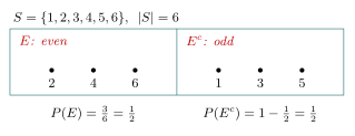
Figure 227: The sample space for one roll of a die, split into the event \(E\), the roll is even, and its complement \(E^c\), the roll is odd. Every outcome lies in exactly one of the two parts. With six equally likely outcomes, \(P(E) = |E| / |S| = 3/6\), and since the two parts fill the whole sample space, \(P(E^c) = 1 - P(E)\).
Equally likely outcomes
If \(S\) is a finite sample space in which every outcome is equally likely, the probability of an event \(E \subseteq S\) is \[P(E) = \frac{|E|}{|S|} = \frac{\text{number of outcomes in } E}{\text{total number of outcomes}}.\]
Wording such as “chosen at random”, “a randomly chosen permutation”, “a fair die” or “shuffled” signals equally likely outcomes. Some consequences come straight from the formula:
- \(0 \le P(E) \le 1\), since \(0 \le |E| \le |S|\).
- \(P(\emptyset) = 0\) and \(P(S) = 1\): an impossible event and a certain one.
- A probability is often quoted as a percentage: \(\frac79 = 0.777\ldots \approx 77.8\%\).
The outcomes must really be equally likely. Roll two dice and ask for the probability that they add to 7. The sums \(2, 3, \dots, 12\) are eleven outcomes, but they are not equally likely, so \(\frac{1}{11}\) is wrong. The equally likely outcomes are the 36 ordered pairs \((1, 1), (1, 2), \dots, (6, 6)\), of which 6 add to 7: \((1,6), (2,5), (3,4), (4,3), (5,2), (6,1)\). So the probability is \(\frac{6}{36} = \frac16\). Choosing a sample space whose outcomes are equally likely is the first step of every problem.
Probability by counting
- Decide what one outcome is, and make sure all outcomes are equally likely. A committee is an unordered selection, a permutation is an ordered arrangement, a password is an ordered selection with repeats (counting-selections).
- Count the sample space, \(|S|\).
- Count the event, \(|E|\), with the same kind of outcome. If \(S\) was counted as unordered selections, \(E\) must be too.
- Divide, and simplify the fraction before turning it into a decimal.
Step 3 is where the counting tools come in: forcing part of the outcome, splitting into categories, gluing objects that must sit together, and the complement.
The complement
For any event \(E\) in a finite sample space \(S\) with equally likely outcomes, \[P(E^c) = 1 - P(E), \qquad\text{equivalently}\qquad P(E) = 1 - P(E^c).\]
Why. \(E\) and \(E^c\) split \(S\) into two disjoint parts, so \(|E^c| = |S| - |E|\) by the difference rule (counting-principles). Dividing by \(|S|\),
\[P(E^c) = \frac{|S| - |E|}{|S|} = 1 - \frac{|E|}{|S|} = 1 - P(E).\]
When to use it. When the event is easier to describe by what it rules out.
- “At least one” has opposite “none”, a single case. \(P(\text{at least one}) = 1 - P(\text{none})\).
- “Not next to each other” has opposite “next to each other”, which is counted by gluing the two objects into one block. \(P(\text{not adjacent}) = 1 - P(\text{adjacent})\).
Worked: a committee with at least one mathematician
A committee of 5 is chosen at random from a group of 25 mathematicians and 25 physicists. What is the probability that at least one mathematician is chosen?
Outcomes. A committee is an unordered selection of 5 of the 50 people, and choosing at random makes every committee equally likely. So
\[|S| = \binom{50}{5} = \frac{50 \cdot 49 \cdot 48 \cdot 47 \cdot 46}{5 \cdot 4 \cdot 3 \cdot 2 \cdot 1} = 2\,118\,760.\]
The complement. “At least one mathematician” means 1, 2, 3, 4 or 5 mathematicians, five cases. Its opposite, “no mathematicians”, is one case: all 5 members are physicists, chosen from the 25 physicists, in
\[\binom{25}{5} = \frac{25 \cdot 24 \cdot 23 \cdot 22 \cdot 21}{5 \cdot 4 \cdot 3 \cdot 2 \cdot 1} = 53\,130\]
ways. Writing \(T = \binom{50}{5}\) for all committees and \(N = \binom{25}{5}\) for those with no mathematicians,
\[\begin{aligned} P(\text{at least one mathematician}) &= \frac{\#(\text{committees with at least one mathematician})}{\#(\text{committees})} = \frac{T - N}{T} = 1 - \frac{N}{T} \\ &= 1 - \frac{\binom{25}{5}}{\binom{50}{5}} = 1 - \frac{53\,130}{2\,118\,760} = 1 - \frac{33}{1316} = \frac{1283}{1316} \\ &\approx 0.9749 \approx 97.5\%. \end{aligned}\]
A quicker route to \(\frac{N}{T}\): the two \(5!\)’s cancel, leaving \(\frac{25 \cdot 24 \cdot 23 \cdot 22 \cdot 21}{50 \cdot 49 \cdot 48 \cdot 47 \cdot 46} = \frac{33}{1316} \approx 0.025\). An all-physicist committee happens about 2.5% of the time.
Figure 228: All \(\binom{50}{5}\) committees of 5 drawn from 25 mathematicians and 25 physicists, split by whether they include a mathematician. The two parts are disjoint and fill the whole set, so the shaded event, at least one mathematician, has probability 1 minus the probability of the small part, an all-physicist committee. The widths are not to scale: the all-physicist committees are only about 2.5% of the total.
Worked: 5 not next to 6
What is the probability that a randomly chosen permutation of \(\{1, 2, \dots, 9\}\) has 5 not next to 6?
Outcomes. A permutation is an ordering of all nine numbers: ordered, no repeats. There are \(|S| = 9!\) of them, all equally likely.
The complement. “5 not next to 6” is awkward to count directly, because where 6 may go depends on where 5 is. Its opposite, “5 next to 6”, is easy. If 5 and 6 are adjacent they appear as 56 or as 65.
- Permutations containing 56. Glue 5 and 6 into a single tile 56. Arranging the permutation is now arranging 8 objects, the tile and the other seven numbers, in a row: \(8!\) ways. Each arrangement of the 8 objects gives exactly one permutation of \(\{1, \dots, 9\}\) with 5 immediately before 6, and every such permutation arises once. (Writing it as \(8 \cdot 7!\), with 8 places the tile can start and \(7!\) orders for the rest, gives the same \(8!\).)
- Permutations containing 65. The same argument with the tile 65: \(8!\).
No permutation contains both, so \(2 \cdot 8!\) permutations have 5 next to 6. Then
\[\begin{aligned} P(\text{5 not next to 6}) &= \frac{9! - 2 \cdot 8!}{9!} = 1 - \frac{2 \cdot 8!}{9 \cdot 8!} = 1 - \frac29 \\ &= \frac{9 - 2}{9} = \frac79 = 0.777\ldots \approx 77.8\%. \end{aligned}\]
In numbers, \(9! = 362\,880\) and \(2 \cdot 8! = 80\,640\), so \(282\,240\) permutations have 5 and 6 apart.
A check by positions. Only the positions of 5 and 6 matter. As an unordered pair they are one of \(\binom92 = 36\) equally likely pairs of positions, and 8 of those pairs are adjacent, \(\{1,2\}, \{2,3\}, \dots, \{8,9\}\). So \(P(\text{adjacent}) = \frac{8}{36} = \frac29\), as before.
Figure 229: Counting permutations of \(1, \dots, 9\) in which 5 and 6 are next to each other. Glue the pair into one tile. With the tile 56 there are 8 objects to arrange, the tile and the seven other numbers, in \(8!\) ways, and each arrangement unglues to a permutation with 5 just before 6. The tile 65 gives another \(8!\), with 6 just before 5. So \(2 \cdot 8!\) of the \(9!\) permutations have 5 next to 6, and the probability that they are apart is \(1 - \frac{2 \cdot 8!}{9!} = \frac79\).
Common mistakes
- Mixing kinds of outcome. If the sample space counts committees as unordered selections, the event must too. Counting \(|S|\) as \(\binom{50}{5}\) and \(|E|\) as ordered selections gives a “probability” up to \(5! = 120\) times too large, and often bigger than 1.
- Outcomes that aren’t equally likely. The sum of two dice is not uniform on \(2, \dots, 12\); use the 36 ordered pairs.
- Forgetting one of the orders when gluing. “Next to” includes both 56 and 65. Counting only one gives \(P(\text{adjacent}) = \frac19\) and the wrong answer \(\frac89\).
- Labelling the complement as the event. \(\frac{N}{T}\) is the probability of no mathematicians, about 2.5%; \(1 - \frac{N}{T}\) is the probability of at least one, about 97.5%. Name each quantity before computing it.
- Rounding too early. Keep the exact fraction, here \(\frac{1283}{1316}\) and \(\frac79\), and round only at the end.
- A probability outside \([0, 1]\). It always means a slip in one of the counts.
See also
- counting-selections — the four kinds of selection, restrictions, gluing, and counting “at least” through the complement
- counting-principles — the multiplication, addition and difference rules
- binomial-coefficients — \(\binom{n}{r}\), its symmetry and identities
- inclusion-exclusion — counting, and so finding the probability of, a union of events that overlap
- sets-and-set-notation — events are subsets, and \(E^c\) is the set complement
- 2026-10-19-probability-binomial-coefficients — Lecture 31
- practice-problems — §39, with full worked solutions
Proof Techniques — Direct, Counterexample, Contradiction, Contraposition
The four methods for establishing (or demolishing) a statement of the form \(\forall x \in D, P(x) \to Q(x)\), plus the definitions every proof in this course is expected to unfold.
Definitions to prove from
Proofs are written by demonstrating facts using the definitions — so these have to be at your fingertips. Each is a biconditional: it can be used in either direction.
| Term | Definition |
|---|---|
| \(n\) is even | \(n = 2k\) for some integer \(k\) |
| \(n\) is odd | \(n = 2k + 1\) for some integer \(k\) (equivalently \(n = 2k - 1\) for some integer \(k\)) |
| \(n\) is prime | \(n \in \mathbb{Z}\), \(n > 1\), and \(\forall r, s \in \mathbb{Z}^+\), if \(n = rs\) then (\(r = 1\) and \(s = n\)) or (\(r = n\) and \(s = 1\)) |
| \(n\) is composite | \(n \in \mathbb{Z}\), \(n > 1\), and \(\exists r, s \in \mathbb{Z}^+\) such that \(n = rs\) and \(1 < r < n\) and \(1 < s < n\) |
| \(r\) is rational | \(\exists a, b \in \mathbb{Z}\) such that \(r = \frac{a}{b}\) and \(b \neq 0\) |
| \(d \mid n\) | \(d \neq 0\) and \(n = dk\) for some integer \(k\) |
Two facts used constantly, and worth naming explicitly when you lean on them:
- Fact: the sum, difference, and product of integers is an integer.
- Fact: every integer is either even or odd.
Parity
Almost every early proof in this course turns on whether something is even or odd, so the consequences of those two definitions are worth having ready rather than re-deriving:
| Result | |
|---|---|
| \(\text{even} + \text{even}\), \(\text{odd} + \text{odd}\) | even |
| \(\text{even} + \text{odd}\) | odd |
| \(\text{even} \times\) anything | even |
| \(\text{odd} \times \text{odd}\) | odd |
| consecutive integers | opposite parity — so two integers two apart share their parity |
Each row follows from the two definitions by a one-line substitution. Subtraction behaves like addition throughout, since \(m - n\) and \(m + n\) differ by \(2n\).
The “two apart” row is the whole content of the warm-up in 2026-07-27-welcome-and-intro-problems, where consecutive \(p < q < r\) forces \(p + r\) to be even and \(r - p\) to be exactly \(2\), while \(pr\) is free to be either.
Prime vs. not-prime. For \(n \in \mathbb{Z}^{>1}\), “\(n\) is not prime” means “\(n\) is composite”. For \(n \in \mathbb{Z}\) generally, “\(n\) is not prime” means “\(n\) is composite or \(n \leq 1\)” — the integers split into \(\mathbb{Z}^{\leq 1}\), \(\mathbb{Z}^{\text{prime}}\), and \(\mathbb{Z}^{\text{composite}}\), and \(1\) and everything below it is in none of the latter two. This is why \(n = 1\) is the standard counterexample to “every positive integer is prime or composite”.
Warning: don’t assume something that seems like an “obvious fact” until you have proven it, or can name the lecture or pre-work video it was proved in.
The four methods
All four target \(\forall x \in D, P(x) \to Q(x)\). Recall the truth table for \(p \to q\) — the only row that makes it false is \(p\) true, \(q\) false:
| \(p\) | \(q\) | \(p \to q\) |
|---|---|---|
| T | T | T |
| T | F | F |
| F | T | T |
| F | F | T |
Every method below is a different way of attacking that one row.
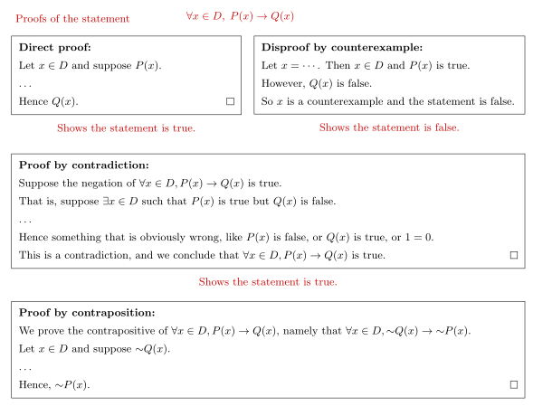
Figure 230: The skeletons of the four methods for a statement of the form ∀x ∈ D, P(x) → Q(x). Three of the four establish the statement and one demolishes it, which is what the red verdict lines record.
Direct proof (shows the statement is true)
Let \(x \in D\) and suppose \(P(x)\). \(\dots\) Hence \(Q(x)\). \(\square\)
Why suppose \(P(x)\) is true, when \(P(x) \to Q(x)\) holds anyway if \(P(x)\) is false? Because the only case that could make the statement false is \(P(x)\) true and \(Q(x)\) false. Ruling that out is the whole job — the \(P(x)\)-false rows are true for free.
Disproof by counterexample (shows the statement is false)
Let \(x = \cdots\). Then \(x \in D\) and \(P(x)\) is true. However, \(Q(x)\) is false. So \(x\) is a counterexample and the statement is false.
A counterexample to \(p \to q\) needs \(p\) true and \(q\) false — a value where the hypothesis fails proves nothing.
Proof by contradiction (shows the statement is true)
Suppose the negation of \(\forall x \in D, P(x) \to Q(x)\) is true. That is, suppose \(\exists x \in D\) such that \(P(x)\) is true but \(Q(x)\) is false. \(\dots\) Hence something that is obviously wrong, like \(P(x)\) is false, or \(Q(x)\) is true, or \(1 = 0\). This is a contradiction, and we conclude that \(\forall x \in D, P(x) \to Q(x)\) is true. \(\square\)
The set-up comes straight from quantified-statements: the negation of \(\forall x \in D, P(x) \to Q(x)\) is \(\exists x \in D\) such that \(P(x) \land \sim Q(x)\).
Useful negations to have ready (see logical-equivalence-laws):
\[\sim(p \lor q) \equiv \sim p \land \sim q \qquad \sim(p \land q) \equiv \sim p \lor \sim q \qquad \sim(p \to q) \equiv p \land \sim q\]
Proof by contraposition (shows the statement is true)
We prove the contrapositive of \(\forall x \in D, P(x) \to Q(x)\), namely that \(\forall x \in D, \sim Q(x) \to \sim P(x)\). Let \(x \in D\) and suppose \(\sim Q(x)\). \(\dots\) Hence, \(\sim P(x)\). \(\square\)
This is valid because \(p \to q \equiv \sim q \to \sim p\) (see conditional-statements).
Choosing a method
- Contradiction is the most versatile, but it needs more set-up, so a direct proof is often easier when one is available.
- Contraposition is the natural choice when \(\sim Q(x)\) gives you something concrete to work with and \(P(x)\) doesn’t — typically when the conclusion is a negative statement (“\(r\) is irrational”, “\(n\) is odd”) whose negation is a definition you can expand.
- Contradiction vs. contraposition: a contraposition proof is a contradiction proof that never actually needs the assumption \(P(x)\) — you derive \(\sim P(x)\) from \(\sim Q(x)\) alone. If your “contradiction” proof only ever uses the \(\sim Q(x)\) half of the assumption, write it as a contraposition instead.
- Counterexample vs. contradiction: counterexample is a disproof, contradiction is a proof. They are not variants of each other.
Worked comparisons on the same statements live in the lecture notes: 2026-08-13-proof-by-contradiction proves \(\forall n \in \mathbb{Z}\), if \(n\) is odd then \(3n+2\) is odd both directly and by contradiction, and 2026-08-13-proof-by-contraposition works through statements where one method gets stuck and another doesn’t.
Worked examples
Direct proof
\(\forall n \in \mathbb{Z}\), if \(n\) is odd then \(3n + 2\) is odd.
Let \(n \in \mathbb{Z}\) and suppose \(n\) is odd. Then \(n = 2k + 1\) for some \(k \in \mathbb{Z}\). Now \[3n + 2 = 3(2k+1) + 2 = 6k + 5 = 2(3k + 2) + 1.\] Since \(k \in \mathbb{Z}\), we have \(3k + 2 \in \mathbb{Z}\), and hence \(3n + 2\) is odd. \(\square\)
For any integer \(x\), if \(x + 6 = 4y\) for some integer \(y\), then \(\frac{x}{2}\) is an odd integer.
Let \(x \in \mathbb{Z}\) and suppose \(x + 6 = 4y\) for some \(y \in \mathbb{Z}\). Then \(x = 4y - 6 = 2(2y - 3)\), so \[\frac{x}{2} = \frac{2(2y-3)}{2} = 2y - 3 = 2(y - 1) - 1.\] Since \(y \in \mathbb{Z}\) we have \(2y - 3 \in \mathbb{Z}\), so \(\frac{x}{2} \in \mathbb{Z}\); and \(y - 1 \in \mathbb{Z}\), so by definition \(\frac{x}{2}\) is odd. \(\square\)
The sum of any pair of even integers is even.
Let \(m, n \in \mathbb{Z}\) be even. Then \(m = 2k\) and \(n = 2\ell\) for some \(k, \ell \in \mathbb{Z}\). Hence \(m + n = 2k + 2\ell = 2(k + \ell)\), which is even. \(\square\)
\(\forall n \in \mathbb{Z}^+\), if \(n \geq 4\) then \(2n^2 - 5n + 2\) is composite.
Suppose \(n \in \mathbb{Z}^+\) and \(n \geq 4\). Factor \(2n^2 - 5n + 2 = (2n - 1)(n - 2)\). Since \(n \geq 4\), we have \(2n - 1 \geq 7\) and \(n - 2 \geq 2\), so both factors are integers greater than \(1\). Hence the expression is composite. \(\square\)
Disproof by counterexample
- For all integers \(m\) and \(n\), if \(2m + n\) is odd then \(m\) and \(n\) are both odd. Counterexample \(m = 4, n = 5\): \(2(4) + 5 = 13\) is odd, but \(m\) is even. (Not \(m=3, n=5\) — there the conclusion holds; not \(m=3,n=6\) or \(m=4,n=6\) — there the hypothesis fails.)
- \(\forall n \in \mathbb{Z}^{\geq 2}\), \(n\) is composite or \(n + 1\) is composite. Take \(n = 2\): both \(2\) and \(3\) are prime.
- For each integer \(n \geq 2\), the product of the first \(n\) primes minus \(1\) is prime. Take \(n = 4\): \(2 \cdot 3 \cdot 5 \cdot 7 - 1 = 209 = 11 \cdot 19\), composite.
- \(\forall x, y \in \mathbb{R}\), if \(y^2 > x^2\) then \(y > x\). Take \(x = 1, y = -2\): \(4 > 1\) but \(-2 \not> 1\).
- \(\forall x \in \mathbb{R}, \lfloor x^2 \rfloor = \lfloor x \rfloor^2\). Take \(x = \frac{3}{2}\): \(\lfloor \frac{9}{4} \rfloor = 2\) but \(\lfloor \frac{3}{2} \rfloor^2 = 1\). (See modular-arithmetic for the floor function.)
Disproof by proving the negation
When the statement to disprove is existential, a single counterexample isn’t available — you must prove the universal negation.
\(\exists n \in \mathbb{Z}^+\) such that \(n^2 + 5n + 6\) is prime. This is false; the negation is \(\forall n \in \mathbb{Z}^+\), \(n^2 + 5n + 6\) is composite.
Let \(n \in \mathbb{Z}^+\). Now \(n^2 + 5n + 6 = (n+2)(n+3)\). Since \(n \geq 1\) we have \(n + 2 > 1\) and \(n + 3 > 1\), so \(n^2 + 5n + 6\) is composite. \(\square\)
(Because \(n \geq 1\) forces \(n^2 + 5n + 6 \geq 2\), “not prime” here does mean “composite”.)
There is an even integer \(n\) such that \(5n - 4\) is prime. False; prove \(\forall n \in \mathbb{Z}^{\text{even}}\), \(5n - 4\) is not prime.
Suppose \(n\) is even, so \(n = 2k\) for some \(k \in \mathbb{Z}\). Then \(5n - 4 = 10k - 4 = 2(5k - 2)\), which is even. The only even prime is \(2\); if \(2(5k-2) = 2\) then \(k = \frac{3}{5} \notin \mathbb{Z}\). Therefore \(5n - 4\) is not prime. \(\square\)
Proof by contradiction
\(\forall m, n \in \mathbb{Z}\), if \(mn\) is even, then \(m\) is even or \(n\) is even.
Suppose \(\exists m, n \in \mathbb{Z}\) such that \(mn\) is even and both \(m\) and \(n\) are odd. Since \(m\) is odd, \(m = 2k+1\) for some \(k \in \mathbb{Z}\); since \(n\) is odd, \(n = 2\ell + 1\) for some \(\ell \in \mathbb{Z}\) — a new variable, since \(m\) and \(n\) need not be equal. Now \[mn = (2k+1)(2\ell+1) = 4k\ell + 2k + 2\ell + 1 = 2(2k\ell + k + \ell) + 1.\] Since \(k, \ell \in \mathbb{Z}\), \(2k\ell + k + \ell \in \mathbb{Z}\), so \(mn\) is odd. It is impossible for \(mn\) to be both even and odd, a contradiction. Therefore the original statement is true. \(\square\)
\(\forall n \in \mathbb{Z}\), if \(3n^3 - 2\) is odd, then \(n\) is odd.
Suppose the statement is false: \(\exists n \in \mathbb{Z}\) such that \(3n^3 - 2\) is odd and \(n\) is even. Since \(n\) is even, \(n = 2a\) for some \(a \in \mathbb{Z}\). Then \[3n^3 - 2 = 3(2a)^3 - 2 = 24a^3 - 2 = 2(12a^3 - 1).\] Since \(a \in \mathbb{Z}\), \(12a^3 - 1 \in \mathbb{Z}\), so \(3n^3 - 2\) is even — a contradiction. Therefore the original statement is true. \(\square\)
\(\forall m, n \in \mathbb{Z}\), if \(m + n\) is even, then \(m\) and \(n\) are both even or both odd.
Suppose the statement is false. Then \(\exists m, n \in \mathbb{Z}\) such that \(m + n\) is even but exactly one of \(m, n\) is even. Without loss of generality, assume \(m\) is even and \(n\) is odd — the other case (\(m\) odd, \(n\) even) follows because \(m + n = n + m\). Thus \(m = 2a\) for some \(a \in \mathbb{Z}\) and \(n = 2b + 1\) for some \(b \in \mathbb{Z}\). Now \(m + n = 2a + 2b + 1 = 2(a + b) + 1\), and \(a + b \in \mathbb{Z}\), so \(m + n\) is odd. This contradicts the assumption that \(m + n\) is even. Therefore the original statement is true. \(\square\)
For integers \(a\) and \(b\), if \(6a + 3b\) is odd, then \(b\) is odd.
Suppose there exist integers \(a, b\) with \(6a + 3b\) odd and \(b\) even. Then \(b = 2k\) for some \(k \in \mathbb{Z}\), so \(6a + 3b = 6a + 6k = 2(3a + 3k)\), which is even — contradicting that \(6a + 3b\) is odd. \(\square\)
For all positive integers \(x\) and \(y\), \(x^2 - y^2 \neq 1\).
Suppose \(x, y \in \mathbb{Z}^+\) with \(x^2 - y^2 = 1\). Factoring, \(1 = (x-y)(x+y)\). Since \(x, y\) are positive integers we must have \(x - y = 1\) and \(x + y = 1\), so \(2x = 2\) and \(x = 1\); then \(y = 0\), which is not a positive integer — a contradiction. \(\square\)
Proof by contraposition
\(\forall r \in \mathbb{R}\), if \(r^2\) is irrational, then \(r\) is irrational.
We prove the contrapositive: \(\forall r \in \mathbb{R}\), if \(r \in \mathbb{Q}\) then \(r^2 \in \mathbb{Q}\). Suppose \(r \in \mathbb{R}\) with \(r \in \mathbb{Q}\). Then \(r = \frac{a}{b}\) for some \(a, b \in \mathbb{Z}\) with \(b \neq 0\). Now \(r^2 = \frac{a^2}{b^2}\). Since \(a, b \in \mathbb{Z}\) we have \(a^2, b^2 \in \mathbb{Z}\), and \(b^2 \neq 0\) since \(b \neq 0\). So \(r^2 \in \mathbb{Q}\). \(\square\)
\(\forall m, n \in \mathbb{Z}\), if \(mn\) is odd, then \(m\) and \(n\) are both odd.
We prove the contrapositive: \(\forall m, n \in \mathbb{Z}\), if at least one of \(m, n\) is even then \(mn\) is even. Without loss of generality, assume \(m\) is even, so \(m = 2k\) for some \(k \in \mathbb{Z}\). Now \(mn = (2k)n = 2(kn)\), and \(kn \in \mathbb{Z}\), so \(mn\) is even. \(\square\)
For all integers \(a\) and \(b\), if \((ab)^2\) is odd then \(a\) is odd and \(b\) is odd.
Contrapositive: if \(a\) is even or \(b\) is even, then \((ab)^2\) is even. WLOG suppose \(a\) is even, so \(a = 2k\) for some \(k \in \mathbb{Z}\). Then \(ab = 2kb\) and \((ab)^2 = 4k^2b^2 = 2(2k^2b^2)\). Since \(k, b \in \mathbb{Z}\), \(2k^2b^2 \in \mathbb{Z}\), so \((ab)^2\) is even. \(\square\)
For all integers \(x\) and \(y\), if \(x^2(y^2 - 2y)\) is odd then \(x\) and \(y\) are odd.
Contrapositive: if \(x\) is even or \(y\) is even, then \(x^2(y^2 - 2y)\) is even. Here the two cases need separate treatment.
Case 1: \(x\) even. \(x = 2k\) for some \(k \in \mathbb{Z}\), so \(x^2(y^2-2y) = 4k^2(y^2-2y) = 2\big(2k^2(y^2-2y)\big)\), and \(2k^2(y^2-2y) \in \mathbb{Z}\).
Case 2: \(y\) even. \(y = 2\ell\) for some \(\ell \in \mathbb{Z}\), so \(x^2(y^2-2y) = x^2\big(4\ell^2 - 4\ell\big) = 2\big(x^2(2\ell^2 - 2\ell)\big)\), and \(x^2(2\ell^2-2\ell) \in \mathbb{Z}\).
In both cases \(x^2(y^2-2y)\) is even. \(\square\)
For any integer \(n\), \(n^2\) is odd if and only if \(n\) is odd. A biconditional needs both directions, and they want different methods:
(\(\Leftarrow\), direct) Suppose \(n\) is odd, so \(n = 2k+1\). Then \(n^2 = 4k^2 + 4k + 1 = 2(2k^2 + 2k) + 1\) is odd.
(\(\Rightarrow\), contraposition) The contrapositive is: if \(n\) is even then \(n^2\) is even. Suppose \(n = 2k\). Then \(n^2 = 4k^2 = 2(2k^2)\) is even. \(\square\)
This lemma — for all integers \(n\), if \(n^2\) is even then \(n\) is even — is used in the proof that \(\sqrt{2}\) is irrational (see rational-and-irrational-numbers).
Common proof errors
The course explicitly tests spotting these. The seven below are the list given with the practice problems’ §9 Q3 (see practice-problems, where the four proofs you are asked to find the errors in are worked):
- Arguing from examples — a single example never establishes a universal statement. (“\(\forall x \in \mathbb{R}, \exists y \in \mathbb{R}\) s.t. \(xy = 1\). Proof: if \(x = 10\) take \(y = \frac{1}{10}\).” Not a proof — and the statement is false, since \(x = 0\) has no such \(y\).)
- Using the same variable to mean two different things — “let \(m = 2k+1\) and \(n = 2k\)” only proves the case \(m = n + 1\). Use a fresh variable for each quantity.
- Jumping to the conclusion — writing down the definition you need to satisfy and then asserting it holds, without exhibiting the witnesses.
- Assuming what is to be proved — starting from “\(4a + 2b = 2\ell\)” and manipulating both sides assumes the conclusion. Derive the conclusion; don’t begin with it.
- Confusion between what is known and what is to be shown.
- Use of the word any instead of some.
- Misuse of the word if.
One more, not on that list: forgetting to state your assumptions, or forgetting to say where a variable lives (“for some \(r, s \in \mathbb{Z}\)”). Introduce every existential witness with its domain.
See also
- quantified-statements — the negations these proofs are built on
- conditional-statements · logical-equivalence-laws
- 2026-07-27-welcome-and-intro-problems — the parity warm-up, the course’s first proof-shaped problem
- proving-set-properties — the element method, and these techniques applied to sets
- rational-and-irrational-numbers · divisibility-and-factorisation
- practice-problems — §9 Direct Proofs and Counterexamples, with full worked solutions
- practice-problems — §10 Proof by Contradiction, with full worked solutions
- practice-problems — §11 Proof by Contraposition, with full worked solutions
Proving Properties of Sets
Three different ways to prove a statement about sets, when to reach for each, and the set identities the third one runs on. See sets-and-set-notation for the definitions being manipulated and proof-techniques for the general proof shapes underneath.
Three methods
| Method | Useful for | How it works |
|---|---|---|
| Element method | a variety of results about sets | argue about an arbitrary element |
| Laws of logical equivalence | proving two sets are equal | rewrite membership as a logical statement and transform it |
| Set identities | proving two sets are equal | rewrite the set expression itself, citing named identities |
The element method is the general-purpose one — it is the only one of the three whose stated forms reach a containment (\(\subseteq\), \(\subset\)) rather than an equality; the other two are given only for proving that two sets are equal. Those other two are quicker, and the choice between them is yours.
Figure 231: Which method can reach which goal. A containment has only one route open to it; an equality has three, and the two braced as quicker do it in a single chain rather than two separate containment proofs.
The element method
To prove \(S \subseteq T\), consider an arbitrary element \(x \in S\) and show that \(x \in T\).
To prove \(S \subset T\), prove \(S \subseteq T\) and then prove \(\exists\, t \in T\) such that \(t \notin S\).
To prove \(S = T\), prove \(S \subseteq T\) and also prove \(T \subseteq S\).
There is a fourth shape worth naming separately, since it is the one that does not mention two sets at all:
To prove that all elements of a set \(S\) have property \(P\), suppose \(x \in S\) and then prove that \(x\) has property \(P\).
Worked: a containment that is proper
Let \(S = \{x \in \mathbb{Z} \mid x \equiv 2 \;(\mathrm{mod}\; 3)\}\) and \(T = \{x \in \mathbb{Z} \mid x \equiv 5 \;(\mathrm{mod}\; 6)\}\). Prove \(T \subset S\).
Listing a few elements first is a good habit — it tells you which way the containment can possibly go:
\[S = \{\dots, -7, -4, -1, 2, 5, 8, 11, \dots\} \qquad T = \{\dots, -7, -1, 5, 11, \dots\}\]
\(T\) is visibly the sparser set, so \(T \subset S\) is the direction to attempt. The proof has the two parts the definition of \(\subset\) demands:
Proof.
(i) \(T \subseteq S\). Suppose \(t \in T\). Then \(t = 6k + 5\) for some integer \(k\). Thus \[t = 6k + 5 = 3(2k + 1) + 2\] and since \(2k + 1 \in \mathbb{Z}\), we have \(t \equiv 2 \;(\mathrm{mod}\; 3)\), so \(t \in S\). Therefore \(T \subseteq S\).
(ii) The containment is proper. \(2 \in S\) but \(2 \notin T\). Therefore \(T \subset S\). \(\blacksquare\)
Part (i) is a general argument about an arbitrary \(t\); part (ii) is a single exhibited witness. Getting those two registers the right way round is most of the skill — a general claim needs a general argument, a “there exists” needs one example.
Worked: complementation reverses containment
Prove that for all sets \(A\) and \(B\) in some universe \(U\), if \(A \subseteq B\) then \(B^{c} \subseteq A^{c}\).
Proof. Let \(x \in B^{c}\). Then \(x \in U - B\) by definition of complement, and thus \(x \in U\) and \(x \notin B\) by definition of set difference.
Since \(A \subseteq B\) we have: every element in \(A\) is also an element of \(B\). Taking the contrapositive, \[x \notin B \;\Longrightarrow\; x \notin A\] Since \(x \in U\) and \(x \notin A\), by definition of complement \(x \in A^{c}\). Therefore \(B^{c} \subseteq A^{c}\). \(\blacksquare\)
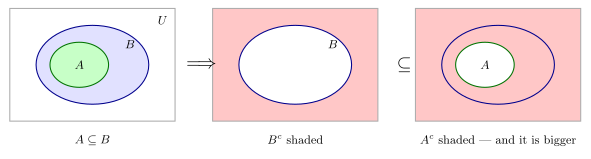
Figure 232: Complementation reverses containment. The smaller set has the larger complement — everything outside B is also outside A, because A was inside B to begin with. The shaded region on the right contains the shaded region on the left.
A picture is not a proof
For all sets \(A\), \(B\), \(C\): \(\;(A - B) \cap (B - A) = \emptyset\). True.
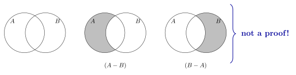
Figure 233: The sets A and B, then A − B shaded, then B − A shaded. The two shaded regions are visibly disjoint, which makes the result believable and is exactly what a proof may not rest on.
The diagrams make the claim obvious, and they are still not a proof. That is a point worth dwelling on, because Venn diagrams are so persuasive:
- A diagram shows one configuration of the sets. The claim is about all sets \(A\), \(B\), \(C\) — including cases the picture does not draw, such as \(A = B\), or either set empty, or one contained in the other.
- The regions in a Venn diagram are drawn as non-empty; the statement has to hold when they are not.
The proof is short and needs no picture: suppose \(x \in (A-B) \cap (B-A)\). Then \(x \in A - B\), so \(x \in A\) and \(x \notin B\); and \(x \in B - A\), so \(x \in B\) and \(x \notin A\). Then \(x \in B\) and \(x \notin B\), a contradiction. So no such \(x\) exists and the intersection is empty. \(\blacksquare\)
Use diagrams to find the answer and to check your intuition. Write the element argument to justify it.
The laws of logical equivalence method
The idea: “\(x \in S\)” is a logical statement, so the laws of logical-equivalence-laws apply to it directly. Write out what membership of \(S\) means, transform it, and read off membership of \(T\) at the end.
Example. Prove that for all sets \(A\) and \(B\), \(\;A - (A - B) = A \cap B\).
\[\begin{aligned} x \in A - (A - B) &\equiv (x \in A) \land \big(x \notin (A-B)\big) && \text{by definition of set difference} \\ &\equiv (x \in A) \land \sim\!\big(x \in (A-B)\big) && \text{by definition of } \notin \\ &\equiv (x \in A) \land \sim\!\big((x \in A) \land (x \notin B)\big) && \text{by definition of set difference} \\ &\equiv (x \in A) \land \big(\sim\!(x \in A) \lor \sim\!(x \notin B)\big) && \text{by De Morgan's law} \\ &\equiv (x \in A) \land \big((x \notin A) \lor (x \in B)\big) && \text{by definition of } \in \text{ and } \notin \\ &\equiv \big((x \in A) \land (x \notin A)\big) \lor \big((x \in A) \land (x \in B)\big) && \text{by the distributive law} \\ &\equiv \mathbf{c} \lor \big((x \in A) \land (x \in B)\big) && \text{by the negation law} \\ &\equiv (x \in A) \land (x \in B) && \text{by the identity law} \\ &\equiv x \in A \cap B && \text{by the definition of } \cap \end{aligned}\]
Two things to copy from the layout. Every line is justified by name — the marks are in the justification column as much as the algebra. And only four of the nine steps are logical manipulation at all: De Morgan, distributive, negation and identity. The other five are definitions translating set language into logic and back — the three at the top, the last one, and the “\(\in\) and \(\notin\)” line, which sits in the middle of the chain rather than at either end.
Note this method proves the equality in one pass, not two. The chain is a string of \(\equiv\), so it reads correctly in both directions — which is what saves you the second containment proof the element method would demand.
Set identities
For all sets \(A\), \(B\) and \(C\) that are subsets of a universal set \(U\):
| Law | (a) | (b) | |
|---|---|---|---|
| 1 | Commutative | \(A \cup B = B \cup A\) | \(A \cap B = B \cap A\) |
| 2 | Associative | \((A \cup B) \cup C = A \cup (B \cup C)\) | \((A \cap B) \cap C = A \cap (B \cap C)\) |
| 3 | Distributive | \(A \cup (B \cap C) = (A \cup B) \cap (A \cup C)\) | \(A \cap (B \cup C) = (A \cap B) \cup (A \cap C)\) |
| 4 | Identity | \(A \cup \emptyset = A\) | \(A \cap U = A\) |
| 5 | Complement | \(A \cup A^{c} = U\) | \(A \cap A^{c} = \emptyset\) |
| 6 | Double Complement | \((A^{c})^{c} = A\) | |
| 7 | Idempotent | \(A \cup A = A\) | \(A \cap A = A\) |
| 8 | Universal Bound | \(A \cup U = U\) | \(A \cap \emptyset = \emptyset\) |
| 9 | De Morgan’s | \((A \cup B)^{c} = A^{c} \cap B^{c}\) | \((A \cap B)^{c} = A^{c} \cup B^{c}\) |
| 10 | Absorption | \(A \cup (A \cap B) = A\) | \(A \cap (A \cup B) = A\) |
| 11 | Complement of \(U\) and \(\emptyset\) | \(U^{c} = \emptyset\) | \(\emptyset^{c} = U\) |
| 12 | Set Difference | \(A - B = A \cap B^{c}\) |
Provided in the exam. These are printed on the MATH1061/MATH7861 Examination Formula Page alongside the laws of logical equivalence — see formula-sheet. They do not need memorising; the marks are in picking the right one and naming it.
The correspondence with logical-equivalence-laws is not a coincidence: \(\cup\) behaves like \(\lor\), \(\cap\) like \(\land\), \({}^{c}\) like \(\sim\), \(U\) like \(\mathbf{t}\) and \(\emptyset\) like \(\mathbf{c}\). Laws 1–11 are the eleven logical equivalences with the symbols swapped, in the same order and under the same names bar the rename of negation to complement — which is precisely why the previous method works. Law 12 is the exception: the formula page’s logical equivalences have no entry corresponding to set difference, which is why it has to be cleared out of the way first.
Law 12 is the one to reach for first in almost any problem containing a minus sign: it converts set difference — which none of the other eleven laws mention — into intersection and complement, which all of them do.
The set identities method
Same result again, this time by transforming the set expression rather than a membership statement.
Prove that for all sets \(A\) and \(B\), \(\;A - (A - B) = A \cap B\).
\[\begin{aligned} A - (A - B) &= A - (A \cap B^{c}) && \text{by the set difference law (12)} \\ &= A \cap (A \cap B^{c})^{c} && \text{by the set difference law (12)} \\ &= A \cap \big(A^{c} \cup (B^{c})^{c}\big) && \text{by De Morgan's law (9b)} \\ &= A \cap (A^{c} \cup B) && \text{by the double complement law (6)} \\ &= (A \cap A^{c}) \cup (A \cap B) && \text{by the distributive law (3b)} \\ &= \emptyset \cup (A \cap B) && \text{by the complement law (5b)} \\ &= A \cap B && \text{by the identity law (4a)} \end{aligned}\]
Seven lines against the previous method’s nine, and no logic notation at all. Two details worth noting:
- Law 12 is applied twice, to the inner difference and then the outer one. Clearing both minus signs before doing anything else is the move that makes the rest routine.
- The last step cites identity law (4a), \(A \cup \emptyset = A\), applied to \(\emptyset \cup (A \cap B)\) — the operands are the other way round, so commutativity (1a) is being used silently. That is normal practice, but it is worth seeing that the step is really two.
Russell’s paradox
When mathematicians wanted to show that all of mathematics could be built on set theory, Bertrand Russell discovered a problem.
Let \(S\) be the set of all sets that are not elements of themselves: \[S = \{A \mid A \text{ is a set and } A \notin A\}\] Is \(S\) an element of itself?
If \(S \in S\), then \(S \notin S\). If \(S \notin S\), then \(S \in S\). So both \(S \in S\) and \(S \notin S\), which is impossible.
The natural objection — surely a set is never an element of itself? — is the right instinct but is not available as an answer, because it is exactly the thing the naive theory fails to guarantee. Nothing in “a set is any collection of objects” forbids self-membership, and \(S\) is built by a rule that looks as legitimate as any other. The contradiction is not in \(S\) being strange; it is in the assumption that every describable collection is a set.
Several ways to define the basic concepts of set theory were found so that Russell’s paradox does not arise — modern axiom systems restrict which collections count as sets. For more detail, read pages 419–421 (5th edition) or 378–380 (4th edition) of the textbook. For more set theory generally, the course to take is MATH3306 Set Theory and Logic.
See also
- sets-and-set-notation — the definitions and operations being proved about
- logical-equivalence-laws — the laws the second method uses, and the source of the set identities
- proof-techniques — contradiction, contraposition and the general proof shapes
- formula-sheet — what is provided in the exam
- inclusion-exclusion — the identities cited by number to prove the three-set counting rule
- functions-on-general-sets — the next thing built on these definitions
- 2026-09-03-set-properties-and-functions — Lecture 18
- practice-problems — §23 Properties of Sets, with full worked solutions
Quantified Statements
Where logical-connectives and conditional-statements deal with whole statements, predicates let us talk about statements whose truth depends on a variable, and quantifiers turn those predicates back into statements that are definitely true or false.
Predicates
A predicate is a sentence with a finite number of variables that becomes a statement when particular values are assigned to those variables.
- Predicates: \(x > 0\), “\(x\) divides \(y\)”.
- Not predicates: “Is it raining?” (a question), “She is happy.” (no objective truth value).
A predicate is written \(P(x)\), and the set of values \(x\) may take is its domain \(D\).
Common domains
| Symbol | Set |
|---|---|
| \(\mathbb{R}\) | real numbers |
| \(\mathbb{Q}\) | rational numbers |
| \(\overline{\mathbb{Q}}\) | irrational numbers (\(\mathbb{R} \setminus \mathbb{Q}\)) |
| \(\mathbb{Z}\) | integers, \(\{\dots, -2, -1, 0, 1, 2, \dots\}\) |
| \(\mathbb{N}\) | natural numbers |
| \(\mathbb{Z}^+\) | positive integers, \(\{1, 2, 3, \dots\}\) |
| \(\mathbb{Z}^{\text{nonneg}} = \mathbb{Z}^{\geq 0}\) | \(\{0, 1, 2, 3, \dots\}\) |
| \(\mathbb{Z}^{\text{even}}\) | \(\{\dots, -4, -2, 0, 2, 4, \dots\}\) |
Nesting: \(\mathbb{N} \subseteq \mathbb{Z} \subseteq \mathbb{Q} \subseteq \mathbb{R}\), with \(\overline{\mathbb{Q}}\) sitting alongside \(\mathbb{Q}\) inside \(\mathbb{R}\).
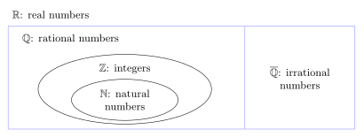
Figure 234: The domains as containers. Each nested label sits inside its own region, with \(\mathbb{R}\) named above the frame, so a claim like ‘every integer is rational’ is read off as one curve lying inside another. The two panels show that the rationals and the irrationals divide the reals between them with nothing in both and nothing left over, which is why ‘x is not rational’ and ‘x is irrational’ say the same thing about a real number — but only about a real number.
Take care with \(\mathbb{N}\) — the diagram deliberately does not say where \(0\) goes. Different sources define \(\mathbb{N}\) as \(\{0, 1, 2, \dots\}\) or \(\{1, 2, 3, \dots\}\), and the course does not pick one. Prefer the unambiguous \(\mathbb{Z}^+\) or \(\mathbb{Z}^{\geq 0}\) in your own writing.
\(\in\) means “belongs to” / “is an element of”; \(\notin\) means “is not an element of”. Note that \(\{\mathbb{Z}\} \neq \mathbb{Z}\) — writing \(x \in \{\mathbb{Z}\}\) says \(x\) is the set \(\mathbb{Z}\), not that \(x\) is an integer.
The two quantifiers
| Symbol | Reads | Associated English words |
|---|---|---|
| \(\forall\) | “for all” | all, every, any, each, none, no |
| \(\exists\) | “there exists” | there is, some, at least one, not all |
- Universal: \(\forall x \in D, P(x)\) — “for all \(x\) in \(D\), \(P(x)\)”.
- Existential: \(\exists x \in D\) such that \(P(x)\) — “there exists an \(x\) in \(D\) such that \(P(x)\)”. “such that” is commonly abbreviated s.t.
Note the punctuation convention: \(\forall\) takes a comma, \(\exists\) takes “such that”.
Translating English to symbols
| English | Symbolic |
|---|---|
| Every rational number is a real number. | \(\forall x \in \mathbb{Q}, x \in \mathbb{R}\) |
| No integer is an irrational number. | \(\forall x \in \mathbb{Z}, x \notin \overline{\mathbb{Q}}\) |
| Some real numbers are rational. | \(\exists x \in \mathbb{R}\) s.t. \(x \in \mathbb{Q}\) |
| Not all rational numbers are integers. | \(\exists x \in \mathbb{Q}\) s.t. \(x \notin \mathbb{Z}\) |
| All prime numbers are odd. | \(\forall x \in P, x\) is odd (with \(P\) the set of primes) |
| If an integer is divisible by 2 then it is divisible by 4. | \(\forall x \in \mathbb{Z},\) if \(2 \mid x\) then \(4 \mid x\) |
Two things to watch:
- “No …” is universal, not existential — “no integer is irrational” becomes \(\forall\), with the predicate negated.
- Sometimes the quantifier is implicit. “If an integer is a square, then it is nonnegative” carries a hidden \(\forall\): \(\forall n \in \mathbb{Z},\) if \(n\) is a square then \(n \geq 0\).
Determining truth
- \(\forall x \in D, P(x)\) is shown false by one counterexample.
- \(\exists x \in D\) s.t. \(P(x)\) is shown true by one example.
The asymmetry matters: a single value can settle a universal statement only in the negative, and an existential statement only in the positive.
\(\exists y \in \mathbb{Z}\) s.t. \(y^2 - y = 0\) is true — choose \(y = 0\) or \(y = 1\). That some other choice (\(y = 2\)) fails is irrelevant; \(\exists\) only asks for one witness. The corresponding universal statement \(\forall y \in \mathbb{Z}, y^2 - y = 0\) is false, and \(y = 2\) is exactly the counterexample that shows it.
\(\forall x \in \mathbb{Z}\), if \(6\) is divisible by \(x\) then \(x = 2\) is false — take \(x = 3\): it’s an integer, \(6\) is divisible by \(3\), but \(3 \neq 2\). (The corrected true statement is \(\forall x \in \mathbb{Z}\), if \(6\) is divisible by \(x\) then \(x = \pm 1, \pm 2, \pm 3\) or \(\pm 6\).)
Negation
Negating a quantified statement flips the quantifier and negates the predicate:
\[\sim\big(\forall x \in D, P(x)\big) \equiv \exists x \in D \text{ s.t. } \sim P(x)\]
\[\sim\big(\exists x \in D \text{ s.t. } P(x)\big) \equiv \forall x \in D, \sim P(x)\]
If the negation of a statement is true, the original is false — so proving the negation is a legitimate way to disprove a statement (see proof-techniques).
When the predicate is itself conditional, negate it with \(\sim(p \to q) \equiv p \land \sim q\) (see logical-equivalence-laws). So the negation of
\[\forall x \in \mathbb{Z}, \text{ if } x^2 > 3 \text{ then } x > 3\]
is \(\exists x \in \mathbb{Z}\) s.t. \(x^2 > 3\) and \(x \leq 3\) — not “if … then …” with an \(\exists\) in front, and not the converse.
A negation is not just “the opposite-sounding statement”
For \(S = \{1, 3, 5, 7\}\), \(\{1,2,3,4\}\), \(\{2,4,6,8\}\):
| \(S\) | \(\forall x \in S, x\) is odd | \(\forall x \in S, x\) is not odd | \(\exists x \in S\) s.t. \(x\) is not odd |
|---|---|---|---|
| \(\{1,3,5,7\}\) | T | F | F |
| \(\{1,2,3,4\}\) | F | F | T |
| \(\{2,4,6,8\}\) | F | T | T |
The first and third columns are exact negations of each other (they disagree in every row). The middle column — “all are not odd” — is not the negation: for \(S = \{1,2,3,4\}\) both it and the original are false.
Worked negations
| Statement | Negation | Which is true |
|---|---|---|
| \(\exists y \in \mathbb{R}\) s.t. \(y^2 < 0\) | \(\forall y \in \mathbb{R}, y^2 \geq 0\) | negation |
| All dogs are white. | Some dog is not white. | negation |
| \(\forall x \in \mathbb{Z}^+, x\) is prime or \(x\) is composite | \(\exists x \in \mathbb{Z}^+\) s.t. \(x\) is neither prime nor composite | negation (\(x = 1\)) |
| \(\forall x \in \mathbb{R}\), if \(x > 2\) then \(x^2 > 4\) | \(\exists x \in \mathbb{R}\) s.t. \(x > 2\) and \(x^2 \leq 4\) | original |
| \(\forall x \in \mathbb{R}\), if \(x^2 > 9\) then \(x \geq 2\) | \(\exists x \in \mathbb{R}\) s.t. \(x^2 > 9\) and \(x < 2\) | negation (\(x = -4\)) |
Multiple quantifiers
Order matters. Read the statement left to right as a game:
- \(\forall x \in X, \exists y \in Y\) s.t. \(P(x,y)\) — “someone gives me an \(x\); can I always then find a \(y\)?” The choice of \(y\) may depend on \(x\).
- \(\exists x \in X\) s.t. \(\forall y \in Y, P(x,y)\) — “is there a single \(x\) that works for every \(y\)?” The \(x\) must be chosen before seeing \(y\).
Both of these happen to be true for \(xy \geq y\) over \(\mathbb{Z}\), but for different reasons:
- \(\forall x \in \mathbb{Z}, \exists y \in \mathbb{Z}\) s.t. \(xy \geq y\) — given \(x\), choose \(y = x\) (since \(x^2 \geq x\) for every integer), or more simply \(y = 0\).
- \(\exists x \in \mathbb{Z}\) s.t. \(\forall y \in \mathbb{Z}, xy \geq y\) — take \(x = 1\), since \(y \geq y\) always.
Where order really bites: \(\forall x \in \mathbb{Z}, \exists y \in \mathbb{Z}\) s.t. \(y = 2x\) is true (given \(x\), take \(y = 2x\)), but \(\forall x \in \mathbb{Z}, \exists y \in \mathbb{Z}\) s.t. \(x = 2y\) is false — take \(x = 3\), and \(y = \tfrac{3}{2} \notin \mathbb{Z}\).
Writing two of the same quantifier
There are three forms:
- \(\exists x \in D\) and \(\exists y \in E \dots\) — the clearest.
- \(\exists x \in D\) and \(y \in E \dots\)
- \(\exists x, y \in D \dots\) — shorthand for the same domain, only correct when both variables share a domain.
All three are acceptable; the first is the safe one.
Negating multiple quantifiers
Flip every quantifier in order, and negate the predicate at the end:
\[\sim\big(\forall x \in X, \exists y \in Y \text{ s.t. } P(x,y)\big) \equiv \exists x \in X \text{ s.t. } \forall y \in Y, \sim P(x,y)\]
The order of the variables never moves — only the quantifiers themselves change. A colour-coded, part-for-part version of this exchange is drawn in 2026-08-06-negation-and-multiple-quantifiers.
Worked examples:
| Statement | Negation | Which is true |
|---|---|---|
| \(\forall x \in \mathbb{R}, \exists y \in \mathbb{R}\) s.t. \(x + y = 0\) | \(\exists x \in \mathbb{R}\) s.t. \(\forall y \in \mathbb{R}, x + y \neq 0\) | original (take \(y = -x\)) |
| \(\forall x \in \mathbb{R}, \exists y \in \mathbb{R}\) s.t. \(xy = 1\) | \(\exists x \in \mathbb{R}\) s.t. \(\forall y \in \mathbb{R}, xy \neq 1\) | negation (\(x = 0\)) |
| \(\exists x \in \mathbb{R}\) s.t. \(\forall y \in \mathbb{R}, xy = 0\) | \(\forall x \in \mathbb{R}, \exists y \in \mathbb{R}\) s.t. \(xy \neq 0\) | original (take \(x = 0\)) |
| \(\exists x \in \mathbb{Z}^+\) s.t. \(\forall y \in \mathbb{Z}^+, x \geq y\) | \(\forall x \in \mathbb{Z}^+, \exists y \in \mathbb{Z}^+\) s.t. \(x < y\) | negation (take \(y = x+1\)) |
| \(\forall x, y \in \mathbb{Z}, \exists z \in \mathbb{Z}\) s.t. \(z = x - y\) | \(\exists x, y \in \mathbb{Z}\) s.t. \(\forall z \in \mathbb{Z}, z \neq x - y\) | original |
| \(\forall r, s \in \mathbb{R}\), if \(rs \in \mathbb{Q}\) then \(r \in \mathbb{Q}\) and \(s \in \mathbb{Q}\) | \(\exists r, s \in \mathbb{R}\) s.t. \(rs \in \mathbb{Q}\) and (\(r \notin \mathbb{Q}\) or \(s \notin \mathbb{Q}\)) | negation (\(r = s = \sqrt{2}\)) |
A negation trap: the negation of “\(\forall x \in \mathbb{Z}, \exists y \in \mathbb{Z}\) s.t. \(x + y\) is odd” is “there exists an integer \(x\) such that for every integer \(y\), \(x + y\) is even”. (The original is true: if \(x\) is odd take \(y = 0\), if \(x\) is even take \(y = 1\).)
See also
- logical-connectives · logical-equivalence-laws · conditional-statements
- proof-techniques — proving and disproving quantified statements
- practice-problems — §6 Quantified Statements, with full worked solutions
- practice-problems — §7 Negation of Quantified Statements, with full worked solutions
- practice-problems — §8 Statements with Multiple Quantifiers, with full worked solutions
Rational & Irrational Numbers
The definitions and closure results that make \(\mathbb{Q}\) a workable object in proofs, plus the classic irrationality argument.
Definitions
\[r \in \mathbb{Q} \iff \exists a, b \in \mathbb{Z} \text{ such that } r = \frac{a}{b} \text{ and } b \neq 0\]
\[r \in \overline{\mathbb{Q}} \iff r \notin \mathbb{Q}\]
\(\overline{\mathbb{Q}} = \mathbb{R} \setminus \mathbb{Q}\) is the set of irrational numbers. The barred symbol is what this course writes, not \(\mathbb{R} \setminus \mathbb{Q}\). Figure 235 shows how the four sets sit together.
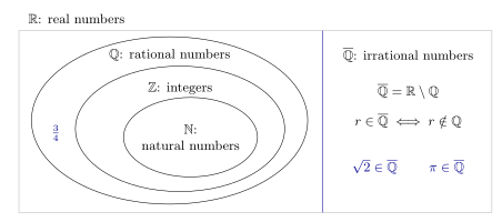
Figure 235: The number systems as nested closed curves with each name written inside its own region, and the irrationals in their own panel because they are the part of the reals that is left over rather than a set that contains any of the others. The three examples are in blue. Two things to read off it — every integer is rational (it is n/1), and no number is in both panels, which is exactly what the definition of the bar says. The course leaves open whether N contains 0, so nothing here should be read as settling that.
Note the definition is existential: to show \(r\) is rational you must exhibit integers \(a\) and \(b\) with \(b \neq 0\). Nearly every proof below ends by checking three things — the numerator is an integer, the denominator is an integer, and the denominator is non-zero.
Fact: every rational number can be written as a fraction in lowest terms (numerator and denominator have no common factors).
Why irrationality statements want contradiction or contraposition
“\(r\) is irrational” is a negative statement — \(r \notin \mathbb{Q}\) — so a direct proof has nothing to unfold. Assuming the negation instead (\(r \in \mathbb{Q}\)) hands you \(r = \frac{a}{b}\) to work with. See proof-techniques for the general shape, and the collected verdicts in 2026-08-13-proof-by-contraposition for which method works on each statement.
Concretely, for the sum of any rational number and any irrational number is irrational:
- Symbolically: \(\forall r, s \in \mathbb{R}\), if \(r \in \mathbb{Q}\) and \(s \in \overline{\mathbb{Q}}\) then \(r + s \in \overline{\mathbb{Q}}\) — or equivalently \(\forall r \in \mathbb{Q}\) and \(\forall s \in \mathbb{R}\), if \(s \in \overline{\mathbb{Q}}\) then \(r + s \in \overline{\mathbb{Q}}\).
- Direct proof: suppose \(r \in \mathbb{Q}\) and \(s \in \overline{\mathbb{Q}}\) — and now you’re stuck, because \(s \in \overline{\mathbb{Q}}\) gives you nothing to substitute.
- Contradiction: suppose \(\exists r \in \mathbb{Q}, s \in \mathbb{R}\) with \(s \in \overline{\mathbb{Q}}\) and \(r + s \in \mathbb{Q}\).
- Contraposition: prove \(\forall r \in \mathbb{Q}\) and \(\forall s \in \mathbb{R}\), if \(r + s \in \mathbb{Q}\) then \(s \in \mathbb{Q}\).
Proof by contraposition. Suppose \(r \in \mathbb{Q}\), \(s \in \mathbb{R}\) and \(r + s \in \mathbb{Q}\). Since \(r \in \mathbb{Q}\), \(r = \frac{a}{b}\) for some \(a, b \in \mathbb{Z}\) with \(b \neq 0\). Since \(r + s \in \mathbb{Q}\), \(r + s = \frac{c}{d}\) for some \(c, d \in \mathbb{Z}\) with \(d \neq 0\). Now \[s = (r + s) - r = \frac{c}{d} - \frac{a}{b} = \frac{bc - ad}{bd}.\] Since \(a, b, c, d \in \mathbb{Z}\) we know \(bc - ad \in \mathbb{Z}\) and \(bd \in \mathbb{Z}\); and \(bd \neq 0\) since \(b \neq 0\) and \(d \neq 0\). Thus \(s \in \mathbb{Q}\). \(\square\)
The trick that makes it work is writing the thing you want in terms of the things you have: \(s = (r + s) - r\). The second fraction needs a fresh pair of variables \(c, d\) — nothing relates it to \(a, b\), and reusing them is one of the standard errors in proof-techniques.
Closure results
\(\forall r \in \mathbb{Q}, (2r^2 - 3r + 1) \in \mathbb{Q}\) — direct proof is best here; contraposition gets stuck.
Let \(r \in \mathbb{Q}\), so \(r = \frac{a}{b}\) for some \(a, b \in \mathbb{Z}\) with \(b \neq 0\). Then \[2r^2 - 3r + 1 = \frac{2a^2}{b^2} - \frac{3ab}{b^2} + \frac{b^2}{b^2} = \frac{2a^2 - 3ab + b^2}{b^2}.\] Since \(a, b \in \mathbb{Z}\) we have \(2a^2 - 3ab + b^2 \in \mathbb{Z}\) and \(b^2 \in \mathbb{Z}\), and \(b^2 \neq 0\) since \(b \neq 0\). So \(2r^2 - 3r + 1 \in \mathbb{Q}\). \(\square\)
\(\forall r \in \mathbb{R}\), if \(r^2\) is irrational then \(r\) is irrational. Proved by contraposition in proof-techniques — the contrapositive is “if \(r \in \mathbb{Q}\) then \(r^2 \in \mathbb{Q}\)”, i.e. \(r^2 = \frac{a^2}{b^2}\) with \(a^2, b^2 \in \mathbb{Z}\) and \(b^2 \neq 0\).
For real \(m, n\): if \(m\) is irrational and \(n\) is rational, then \(m - n\) is irrational.
Proof by contradiction. Suppose \(m\) is irrational, \(n\) is rational, but \(m - n\) is rational. Then \(n = \frac{a}{b}\) and \(m - n = \frac{c}{d}\) for integers \(a,b,c,d\) with \(b, d \neq 0\). Since \(m = (m - n) + n\), \[m = \frac{c}{d} + \frac{a}{b} = \frac{bc + ad}{bd},\] with \(bc + ad \in \mathbb{Z}\), \(bd \in \mathbb{Z}\) and \(bd \neq 0\). So \(m\) is rational, contradicting the assumption. \(\square\)
For a real number \(r\): if \(2r^2 - 3r\) is irrational, then \(r\) is irrational.
Proof by contraposition. The contrapositive is: if \(r \in \mathbb{Q}\) then \(2r^2 - 3r \in \mathbb{Q}\). Let \(r = \frac{a}{b}\) with \(a, b \in \mathbb{Z}\), \(b \neq 0\). Then \(2r^2 - 3r = \frac{2a^2 - 3ab}{b^2}\), with integer numerator and non-zero integer denominator. \(\square\)
For all real \(r, s\) and \(n\): if \(r\) is irrational, \(s\) is rational and \(n\) is a positive integer, then \(n(r - s)\) is irrational.
Proof by contradiction. Suppose otherwise: \(r \in \overline{\mathbb{Q}}\), \(s \in \mathbb{Q}\), \(n \in \mathbb{Z}^+\), but \(n(r-s) \in \mathbb{Q}\). Write \(s = \frac{a}{b}\) and \(n(r - s) = \frac{c}{d}\) with \(b, d \neq 0\). Since \(n \neq 0\), \[r = s + \frac{c}{d} \cdot \frac{1}{n} = \frac{a}{b} + \frac{c}{dn} = \frac{adn + bc}{bdn}.\] Here \(adn + bc \in \mathbb{Z}\), \(bdn \in \mathbb{Z}\), and \(bdn \neq 0\) since \(b, d, n\) are all non-zero. So \(r \in \mathbb{Q}\) — a contradiction. \(\square\)
For every rational \(r\), if \(r \neq 0\) then \(r\sqrt{2}\) is irrational. Negation: \(\exists r \in \mathbb{Q}\) such that \(r \neq 0\) and \(r\sqrt{2} \in \mathbb{Q}\).
Proof by contradiction. Suppose the negation holds. Since \(r \in \mathbb{Q}\), \(r = \frac{a}{b}\) for some \(a, b \in \mathbb{Z}\) with \(b \neq 0\), and \(a \neq 0\) because \(r \neq 0\). Since \(r\sqrt{2} \in \mathbb{Q}\), \(r\sqrt{2} = \frac{c}{d}\) for integers \(c, d\) with \(d \neq 0\). Then \[\sqrt{2} = \frac{r\sqrt{2}}{r} = \frac{c}{d} \cdot \frac{b}{a} = \frac{bc}{ad},\] where \(bc \in \mathbb{Z}\), \(ad \in \mathbb{Z}\) and \(ad \neq 0\) (since \(a \neq 0\) and \(d \neq 0\)). So \(\sqrt{2} \in \mathbb{Q}\) — contradicting the theorem below. \(\square\)
\(\sqrt{2}\) is irrational
The set-up needs two ingredients: the lowest-terms fact above, and the lemma for all integers \(n\), if \(n^2\) is even then \(n\) is even (proved by contraposition — see proof-techniques).
Proof by contradiction. Suppose \(\sqrt{2}\) is rational. Then \(\sqrt{2} = \frac{a}{b}\) for some \(a, b \in \mathbb{Z}\) with \(b \neq 0\), and we may assume \(\frac{a}{b}\) is in lowest terms.
Squaring, \(2 = \frac{a^2}{b^2}\), so \(a^2 = 2b^2\) and thus \(a^2\) is even. By the lemma, \(a\) is even, so \(a = 2\ell\) for some \(\ell \in \mathbb{Z}\).
Substituting: \(2b^2 = a^2 = (2\ell)^2 = 4\ell^2\), so \(b^2 = 2\ell^2\) and \(b^2\) is even. By the lemma again, \(b\) is even.
But now \(a\) and \(b\) are both even, so they share the common factor \(2\) — contradicting the assumption that \(\frac{a}{b}\) is in lowest terms. Therefore \(\sqrt{2} \in \overline{\mathbb{Q}}\). \(\square\)
The shape of the argument is easier to hold onto than its algebra (Figure 236).
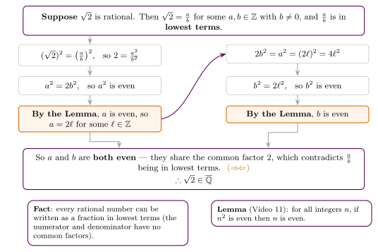
Figure 236: The same proof as a structure. It runs in two halves that use the lemma once each (orange): the left half squeezes ‘a is even’ out of the assumption, and the substitution a = 2l feeds the right half, which gets ‘b is even’. Neither half is a contradiction on its own — the contradiction only appears when both land together and the fraction turns out not to have been in lowest terms after all. That is why the lowest-terms assumption has to be made in the very first line: it is the thing the two halves eventually collide with. The two boxes at the bottom state the Fact and the Lemma.
Neither a direct proof nor a contraposition proof gets off the ground here: the statement isn’t a conditional with a usable hypothesis, so contradiction is the only one of the three that has anywhere to start.
See also
- proof-techniques — direct / counterexample / contradiction / contraposition
- 2026-08-13-proof-by-contraposition — Lecture 9
- quantified-statements
- divisibility-and-factorisation
- practice-problems — §12 Rational Numbers, with full worked solutions
Recursive Definitions
Defining a sequence, or a set, by saying how to build its members out of members you already have. See sequences-and-summations for the other ways to define a sequence, and strong-induction-and-the-well-ordering-principle for the proof method that recursive definitions almost always call for.
Recursively defined sequences
To define a sequence recursively, two things are needed:
- Initial conditions — the values of some number of initial terms of the sequence.
- A recurrence relation — a formula specifying how to calculate the value of a term of the sequence from the values of one or more previous terms.
Neither half is optional, and the same recurrence relation with different initial conditions can give a completely different sequence:
| Definition | Sequence |
|---|---|
| \(a_1 = 2\) and \(a_k = 3a_{k-1}\) for each integer \(k \geq 2\) | \(2, 6, 18, 54, \dots\) |
| \(b_1 = 7\) and \(b_k = 3b_{k-1}\) for each integer \(k \geq 2\) | \(7, 21, 63, 189, \dots\) |
The recurrence is identical; only the seed differs, and the two sequences share no terms.
Checking that a sequence satisfies a recurrence
Given an explicit formula and a candidate recurrence, the check is a one-step calculation: assume the formula at \(k-1\), substitute it into the recurrence, and see whether what comes out is the formula at \(k\).
For \(b_n = 4n + 3\) and the candidate \(b_k = 4 + b_{k-1}\):
\[b_k = 4 + b_{k-1} = 4 + \big(4(k-1) + 3\big) = 4k + 3 \quad\checkmark\]
For the candidate \(b_k = 4b_{k-1}\), the same substitution gives
\[b_k = 4b_{k-1} = 4\big(4(k-1)+3\big) = 16k - 16 + 3 = 16k - 13 \quad\times\]
which is not \(4k+3\), so that recurrence is not satisfied.
Reading a recursive definition off an explicit formula
This section goes explicit \(\to\) recursive. The reverse trip — recursive \(\to\) explicit, which is the harder and more useful one — is solving-recurrence-relations.
Going the other way — from an explicit formula to a recursive definition — means computing the first few terms, spotting what is done to each term to get the next, then proving the guess.
Factorial. For \(n \in \mathbb{Z}^+\), \(n! = n(n-1)\cdots(2)(1)\), and \(0! = 1\) by definition. Worth memorising: the \(0! = 1\) convention is what makes formulas involving \(n!\) work at \(n = 0\) without a special case.
Example: \(a_n = \dfrac{(-1)^n}{n!}\) for each integer \(n \geq 0\).
The first five terms, and the factor taking each to the next:
\[\underbrace{1}_{a_0} \;\xrightarrow{\;\times -1\;}\; \underbrace{-1}_{a_1} \;\xrightarrow{\;\times -\frac{1}{2}\;}\; \underbrace{\tfrac{1}{2}}_{a_2} \;\xrightarrow{\;\times -\frac{1}{3}\;}\; \underbrace{-\tfrac{1}{6}}_{a_3} \;\xrightarrow{\;\times -\frac{1}{4}\;}\; \underbrace{\tfrac{1}{24}}_{a_4}\]
The multiplier at step \(n\) is \(-\frac{1}{n}\), suggesting \(a_n = -\frac{1}{n}a_{n-1}\). Verifying it against the explicit formula:
Suppose \(a_{n-1} = \dfrac{(-1)^{n-1}}{(n-1)!}\). Then
\[a_n = -\frac{1}{n} \cdot a_{n-1} = \frac{(-1)(-1)^{n-1}}{n \cdot (n-1)!} = \frac{(-1)^n}{n!} \quad\checkmark\]
So the recursive definition is
- initial condition: \(a_0 = 1\)
- recurrence relation: \(a_n = -\dfrac{1}{n}a_{n-1}\) for all \(n \geq 1\)
Note how the recurrence relation’s range starts one past the last initial condition — that is the general rule, and it is what makes the definition cover every term exactly once.
Recursively defined sets
To define a set recursively, three things are needed:
- Base — a statement that certain (usually small) objects belong to the set.
- Recursion — rules on how to build new set objects from those objects already known to be in the set.
- Restriction — a statement saying that all objects in the set come from the Base and the Recursion.
The Restriction is the part that is easy to forget and easy to underrate. Without it the Base and Recursion only say what must be in the set; the Restriction is what says nothing else is, and it is what licenses arguing that a given object is not a member.
The set of all binary strings
A binary string is a sequence of 0’s and 1’s. The set \(B\) of all binary strings is defined recursively:
- Base: the empty string \(\varepsilon\) is in \(B\).
- Recursion: if \(s \in B\), then \(s0 \in B\) and \(s1 \in B\).
- Restriction: nothing is in \(B\) other than objects defined by the Base and the Recursion.
Every string therefore has a build history from \(\varepsilon\), one character at a time — the string 011 is built up as \(\varepsilon \to 0 \to 01 \to 011\). Applying the two rules repeatedly generates a binary tree of strings, and a build history is just a path down it from the root:
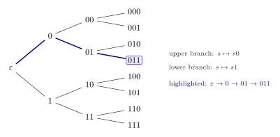
Figure 237: The Recursion applied three times over, drawn the way the lecture drew it: the Base object \(\varepsilon\) at the root on the left, the two rules fanning rightwards as plain segments with no arrowheads, and each node labelled with the string it is. The upper branch appends a 0 and the lower a 1, so the level a string sits at is its length. The highlighted path is added here — the lecture wrote the build history of 011 out as a separate chain rather than marking it on the tree; drawn on the tree it shows what a build history actually is, a route from the Base to the object.
Two things the picture makes plain that the rules alone do not. Every binary string appears exactly once in this tree, at depth equal to its length — so for \(B\) a build history is unique, and there is no ambiguity about how a given string was made. And the tree only ever grows: neither rule shortens a string, so a property that holds at the root and survives both rules holds everywhere below. That is the shape of argument the Restriction licenses, and it is what the next section turns into a method.
Arguing about membership
For a recursively defined set, the two directions of argument look quite different:
- To show an object is in the set, exhibit a build history — a chain from the Base to the object, with each step naming the rule used.
- To show an object is not in the set, find a property that the Base has and that every Recursion rule preserves, and observe the object lacks it. This is an induction over the structure of the set, and it works only because of the Restriction.
See also
- solving-recurrence-relations — the other direction: recursive definition to explicit formula, and proving it
- sequences-and-summations · strong-induction-and-the-well-ordering-principle · mathematical-induction
- counting-principles — \(n!\) as the number of arrangements of \(n\) objects
- 2026-08-31-recursive-definitions — Lecture 15
- practice-problems — §19 Recursive Definitions, with full worked solutions
Reflexive, Symmetric and Transitive Relations
The three properties a relation on a single set can have, what each looks like in an arrow diagram, and how to prove or disprove each one. Relations themselves are defined in relations-on-sets. The lecture is 2026-09-17-relations-reflexivity-symmetry-transitivity.
The definitions
A relation \(\rho\) on a set \(A\) is
(1) reflexive if and only if \(\forall x \in A,\ x \mathrel{\rho} x\).
(2) symmetric if and only if \(\forall x, y \in A,\ x \mathrel{\rho} y \to y \mathrel{\rho} x\).
(3) transitive if and only if \(\forall x, y, z \in A,\ (x \mathrel{\rho} y \text{ and } y \mathrel{\rho} z) \to x \mathrel{\rho} z\).
In the arrow diagram:
- reflexive — every dot has a loop;
- symmetric — every arrow has a return arrow;
- transitive — every path of two arrows has a direct arrow from its start to its end, the short cut.
A relation fails a property when the diagram contains one of the patterns in Figure 238. Each is a witness — one specific element, pair or triple. Nothing more is needed to disprove a “for all”.
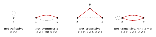
Figure 238: What a failure of each property looks like; any one such pattern in a diagram disproves the property. Not reflexive: one element without a loop. Not symmetric: one arrow whose return is missing. Not transitive: one path of two arrows whose short cut is missing. The fourth panel is the not-transitive pattern with \(z = x\): a round trip \(x \to y \to x\) needs the short cut \(x \to x\), a loop, so two elements joined both ways but without loops already break transitivity. The missing arrows are dashed.
Reading the definitions carefully
Reflexive is about every element. “\(\forall x \in A\)” means a single element without a loop is enough to make a relation not reflexive, even if every other element has one. Disjointness, \(X \mathrel{\rho} Y \leftrightarrow X \cap Y = \emptyset\) on \(\mathcal{P}(\mathbb{Z}^{+})\), is not reflexive, though \(\emptyset \mathrel{\rho} \emptyset\) holds.
Symmetric and transitive are conditional. They say what must happen if certain arrows are present. Where those arrows are absent, the condition holds automatically, by vacuous truth (conditional-statements). This is why a relation with very few arrows can be symmetric and transitive. The empty relation on any set is both, and so is \(\{(1,1)\}\) on \(\{1,2\}\).
\(x\), \(y\), \(z\) need not be different. In the transitive condition, \(z\) may equal \(x\). Then it reads: if \(x \mathrel{\rho} y\) and \(y \mathrel{\rho} x\), then \(x \mathrel{\rho} x\). In a transitive relation, any two elements related both ways both have loops. Three of the transitivity counterexamples in 2026-09-17-relations-reflexivity-symmetry-transitivity use exactly this: \(\{1\}\) and \(\{2\}\) are disjoint both ways but \(\{1\}\) is not disjoint from itself; in Diagram 1 \(b \to a \to b\) exists but the loop at \(b\) does not; and for \(xy \equiv 1 \pmod 7\), \(2 \to 4 \to 2\) exists but \(2 \mathrel{\not\rho} 2\).
Proving and disproving
Each property is a universal statement, so proving it needs a general argument about arbitrary elements, while disproving it needs one witness (quantified-statements, proof-techniques):
| To prove it | To disprove it | |
|---|---|---|
| reflexive | Let \(x \in A\). Show \(x \mathrel{\rho} x\). | Find one \(x \in A\) with \(x \mathrel{\not\rho} x\). |
| symmetric | Let \(x, y \in A\) and suppose \(x \mathrel{\rho} y\). Show \(y \mathrel{\rho} x\). | Find \(x, y \in A\) with \(x \mathrel{\rho} y\) but \(y \mathrel{\not\rho} x\). |
| transitive | Let \(x, y, z \in A\) and suppose \(x \mathrel{\rho} y\) and \(y \mathrel{\rho} z\). Show \(x \mathrel{\rho} z\). | Find \(x, y, z \in A\) with \(x \mathrel{\rho} y\) and \(y \mathrel{\rho} z\) but \(x \mathrel{\not\rho} z\). |
In every proof, unfold the definition of \(\rho\) — turn \(x \mathrel{\rho} y\) into the condition it stands for, work with that, and fold it back up at the end. For a disproof, give specific elements and check each of the stated facts about them.
Worked: \(m \mathrel{\rho} n \leftrightarrow 6 \mid (m - n)\) on \(\mathbb{Z}\)
All three hold. Unfold with the definition of divides (divisibility-and-factorisation): \(m \mathrel{\rho} n\) means \(m - n = 6k\) for some \(k \in \mathbb{Z}\).
- Reflexive. Let \(m \in \mathbb{Z}\). Then \(m - m = 0 = 6 \cdot 0\), so \(6 \mid (m - m)\) and \(m \mathrel{\rho} m\).
- Symmetric. Let \(m, n \in \mathbb{Z}\) with \(m \mathrel{\rho} n\), so \(m - n = 6k\) for some \(k \in \mathbb{Z}\). Then \(n - m = 6(-k)\) and \(-k \in \mathbb{Z}\), so \(6 \mid (n - m)\) and \(n \mathrel{\rho} m\).
- Transitive. Let \(m, n, p \in \mathbb{Z}\) with \(m \mathrel{\rho} n\) and \(n \mathrel{\rho} p\), so \(m - n = 6k\) and \(n - p = 6\ell\) for some \(k, \ell \in \mathbb{Z}\). Adding, \(m - p = 6(k + \ell)\) with \(k + \ell \in \mathbb{Z}\), so \(m \mathrel{\rho} p\).
Its diagram on \(\{0, \dots, 11\}\) is drawn in relations-on-sets. The second divisibility gets a new variable \(\ell\): reusing \(k\) would claim that \(m - n\) and \(n - p\) are the same multiple of 6.
Worked: \(x \mathrel{\rho} y \leftrightarrow x > y\) on \(\mathbb{Z}\)
- Not reflexive. \(0 > 0\) is false, so \(0 \mathrel{\not\rho} 0\).
- Not symmetric. \(1 \mathrel{\rho} 0\) since \(1 > 0\), but \(0 \mathrel{\not\rho} 1\) since \(0 > 1\) is false.
- Transitive. Suppose \(x > y\) and \(y > z\). Then \(x > z\), so \(x \mathrel{\rho} z\).
Worked: divides, on \(\{1, 2, \dots, 6\}\)
\(x \mathrel{\rho} y \leftrightarrow x \mid y\) is reflexive (\(x = x \cdot 1\)), not symmetric (\(1 \mid 2\) but \(2 \nmid 1\)), and transitive: if \(y = xk\) and \(z = y\ell\) then \(z = x(k\ell)\). The diagram shows all three at once.
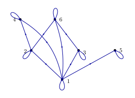
Figure 239: The relation \(x \mid y\) on \({1, 2, \dots, 6}\), with the numbers placed so every arrow points upward. Reflexive: a loop at every number, since each number divides itself. Not symmetric: no arrow comes back down — \(1 \mid 2\), but \(2 \nmid 1\). Transitive: every two-step path has its short cut, such as \(1 \to 2 \to 4\) with the direct arrow \(1 \to 4\). There are 14 arrows: 6 loops and 8 others.
Checking a finite relation from its diagram
For a relation given as a diagram or a list of pairs:
- Reflexive: look for a loop at every element. Any element without one is the witness.
- Symmetric: for each non-loop arrow, look for its return. Any arrow without one is the witness.
- Transitive: for each arrow \(x \to y\), look at every arrow leaving \(y\), say \(y \to z\), and check that \(x \to z\) is there. Include the paths that come back, \(x \to y \to x\), whose short cut is a loop. This is the slow check, and the round trips are where it usually goes wrong.
The same procedure answers “what must be added to make it reflexive, symmetric, transitive”: the missing loops, the missing returns, and the missing short cuts. For transitivity, keep checking after adding, because a new arrow can create new two-step paths. This is worked on Diagram 1 in 2026-09-17-relations-reflexivity-symmetry-transitivity.
The examples side by side
| Relation | on | Reflexive | Symmetric | Transitive |
|---|---|---|---|---|
| \(X \subset Y\) (proper subset) | \(\mathcal{P}(\{1,2,3\})\) | no | no | yes |
| \(X \cap Y = \emptyset\) | \(\mathcal{P}(\mathbb{Z}^{+})\) | no | yes | no |
| Diagram 1 | \(\{a,b,c,d\}\) | no | no | no |
| \(xy \equiv 1 \pmod 7\) | \(\{0, \dots, 6\}\) | no | yes | no |
| \(\{(1,1)\}\) | \(\{1, 2\}\) | no | yes | yes |
| \(6 \mid (m - n)\) | \(\mathbb{Z}\) | yes | yes | yes |
| \(x > y\) | \(\mathbb{Z}\) | no | no | yes |
| \(x \mid y\) | \(\{1, \dots, 6\}\) | yes | no | yes |
The first five are worked in 2026-09-17-relations-reflexivity-symmetry-transitivity; the other three are worked above. The three properties are independent, and most of the eight combinations appear here. Relations with all three, like \(6 \mid (m - n)\), are equivalence relations (equivalence-relations). Relations like \(x \mid y\) — reflexive and transitive, with no two different elements related both ways — are partial orders (partial-order-relations). Those are the next two topics in the course.
Symmetric and transitive do not make reflexive
Claim. If a relation \(\rho\) on a set \(A\) is both symmetric and transitive, then \(\rho\) is reflexive. — False.
Counterexample. \(A = \{1, 2\}\), \(\rho = \{(1,1)\}\). Symmetric: the only pair is \((1,1)\), whose reverse is itself. Transitive: the only two-step path is \(1 \to 1 \to 1\), whose short cut \((1,1)\) is present. Not reflexive: \(2 \mathrel{\not\rho} 2\).
The tempting “proof” goes: let \(x \in A\); take \(y\) with \(x \mathrel{\rho} y\); by symmetry \(y \mathrel{\rho} x\); by transitivity \(x \mathrel{\rho} x\). Every step is valid except the second. Nothing guarantees there is any \(y\) with \(x \mathrel{\rho} y\). The element 2 in the counterexample is related to nothing, so there is nothing to start the argument from. Adding the missing hypothesis makes the claim true:
If \(\rho\) is symmetric and transitive, and for each \(x \in A\) there is some \(y \in A\) with \(x \mathrel{\rho} y\), then \(\rho\) is reflexive.
The proof is the tempting argument above, now legitimate. The picture is the right-hand panel of 2026-09-17-relations-reflexivity-symmetry-transitivity.
See also
- relations-on-sets — relations as sets of pairs, the notation, arrow diagrams
- equivalence-relations · partial-order-relations — the two kinds of relation built from these properties, the second with antisymmetry in place of symmetry
- quantified-statements · proof-techniques — why a “for all” needs a general argument and its negation needs a witness
- conditional-statements — vacuous truth, which is why sparse relations are often symmetric and transitive
- sets-and-set-notation — the proper-subset relation, and why it has no loops
- 2026-09-17-relations-reflexivity-symmetry-transitivity — Lecture 23
- practice-problems — §30, with full worked solutions
Relations on Sets
A relation records which elements are related to which, and nothing more: any set of ordered pairs. Functions are the special relations with exactly one partner for each input. The properties a relation on one set can have are in reflexive-symmetric-and-transitive-relations. The lecture is 2026-09-17-relations-reflexivity-symmetry-transitivity.
The definition
Any subset \(\rho\) of \(A \times B\) is a binary relation from \(A\) to \(B\).
A relation on a set \(A\) is a binary relation from \(A\) to \(A\), that is, a subset of \(A \times A\).
If \((x, y) \in \rho\) we write \(x \mathrel{\rho} y\) and read it “\(x\) is related in \(\rho\) to \(y\)”. If \((x,y) \notin \rho\) we write \(x \mathrel{\not\rho} y\). The two notations mean exactly the same thing and either is fine in an answer. Relations are usually named with Greek letters: \(\rho\) (rho), \(\sigma\) (sigma), \(\tau\) (tau).
Order matters. \((1,0)\) and \((0,1)\) are different pairs, so \(1 \mathrel{\rho} 0\) and \(0 \mathrel{\rho} 1\) are different statements, and one can hold without the other. The first coordinate is where an arrow starts, and the second is where it ends.
For example, with \(A = \{1,2,3,4\}\) and \(B = \{0,2,4,6,8\}\), \[\rho = \{(1,0), (3,4), (4,0), (4,4), (4,6)\}\] is a relation from \(A\) to \(B\): \(1 \mathrel{\rho} 0\), \(3 \mathrel{\rho} 4\), \(4 \mathrel{\rho} 0\), \(4 \mathrel{\rho} 4\), \(4 \mathrel{\rho} 6\), and nothing else is related.
Functions are relations
The definition of a function (functions-on-general-sets) is the definition of a relation with one extra condition:
A subset \(f\) of \(A \times B\) is a function from \(A\) to \(B\) if for each \(a \in A\), there is a unique \(b \in B\) such that \((a,b) \in f\).
So every function is a relation, and a relation is not necessarily a function. A relation may give an element of \(A\) no partner, or several; a function must give each exactly one. Written as a relation, \(f(a) = b\) is just \(a\,f\,b\), since \(f(a) = b \leftrightarrow (a,b) \in f\).
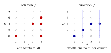
Figure 240: A relation is a choice of points from the grid \(A \times B\). Each column is an element of \(A\) and each row an element of \(B\), and the filled points are the pairs in the relation. Left: the relation \(\rho\) is any choice of points — column 2 is empty, column 4 has three. Right: a function \(f\) is a choice with exactly one point in every column, the unique \(b\) for each \(a\). Nothing restricts the rows in either: in \(f\), row 4 has two points and rows 6 and 8 have none.
Relations defined by a condition
Listing pairs only works for small finite sets. Usually a relation on \(A\) is defined by a condition on \(x\) and \(y\):
- \(x \mathrel{\rho} y \leftrightarrow x > y\) for all \(x, y \in A\);
- \(X \mathrel{\rho} Y \leftrightarrow X \cap Y = \emptyset\) for all \(X, Y \in A\) (here \(A\) is a set of sets, such as \(\mathcal{P}(\mathbb{Z}^{+})\));
- \(m \mathrel{\rho} n \leftrightarrow 6 \mid (m - n)\) for all \(m, n \in A\);
- \(x \mathrel{\rho} y \leftrightarrow xy \equiv 1 \pmod 7\) on \(\{0, 1, \dots, 6\}\).
To decide whether a particular pair is related, substitute and check. \(5 \mathrel{\rho} 2\) under \(x > y\) because \(5 > 2\), and \(2 \mathrel{\not\rho} 5\). Under \(6 \mid (m-n)\), \(13 \mathrel{\rho} 1\) because \(13 - 1 = 12 = 6 \cdot 2\), and \(13 \mathrel{\not\rho} 2\). The relation is the set of all pairs that pass: \(\rho = \{(x,y) \in A \times A : x > y\}\).
Arrow diagrams
A relation on a finite set is drawn as an arrow diagram, also called a directed graph: one dot per element, and an arrow from \(x\) to \(y\) for each pair \((x,y) \in \rho\). An arrow from an element to itself is a loop. The two drawings of a relation on \(A\) are compared in 2026-09-17-relations-reflexivity-symmetry-transitivity. With two copies of \(A\) side by side, as for a function, loops become horizontal arrows and are easy to miss. With a single copy of \(A\), loops, arrows in both directions and paths of two arrows can all be seen at a glance, and those are what the properties of relations are about.
Reading a diagram back into pairs: each arrow is one pair, loops included. Forgetting the loops is the usual slip.
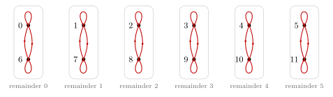
Figure 241: The relation \(m \mathrel{\rho} n \leftrightarrow 6 \mid (m-n)\) on \({0, 1, \dots, 11}\), drawn with a single copy of the set. Two numbers are related exactly when they leave the same remainder on division by 6, so the diagram falls apart into six separate pieces, one per remainder: each number has a loop, since \(6 \mid 0\), and each pair such as 1 and 7 is joined both ways, since \(7 - 1\) and \(1 - 7\) are both multiples of 6. Nothing joins different pieces. A diagram that splits into clusters like this marks a special kind of relation, the equivalence relations.
Common mistakes
- Treating a relation like a function. \(\rho(x)\) means nothing. A relation can have many partners for \(x\), or none, so there is no “value” to name. Write \(x \mathrel{\rho} y\) or \((x,y) \in \rho\).
- Reversing the pair. \(x \mathrel{\rho} y\) is the arrow from \(x\) to \(y\). Under \(x > y\), \(5 \mathrel{\rho} 2\) but not \(2 \mathrel{\rho} 5\).
- Dropping loops when reading pairs off a diagram, or when drawing one.
- Forgetting the set. A relation is on a particular set. “\(xy \equiv 1 \pmod 7\)” on \(\{0, \dots, 6\}\) has 6 pairs, on \(\mathbb{Z}\) infinitely many. Always state or check the set.
See also
- reflexive-symmetric-and-transitive-relations — the three properties, and how to prove or disprove each
- equivalence-relations · partial-order-relations — the two kinds of relation the course goes on to study, and hasse-diagrams, the arrow diagram of a partial order cut down
- functions-on-general-sets — functions as relations with exactly one partner per input
- sets-and-set-notation — Cartesian products and power sets, the raw material of relations
- modular-arithmetic — congruence, the source of relations like \(6 \mid (m - n)\)
- [graphs] — dots joined by edges without arrows, where a loop is an edge with one endpoint and adds 2 to a degree
- 2026-09-17-relations-reflexivity-symmetry-transitivity — Lecture 23
- practice-problems — §29, with full worked solutions
Sample Mid-Semester Exams
Two sample papers, both Semester Two Sample Mid-Semester Examinations, 2021, identically shaped. They are the only guide to the format of the real in-semester exam (20%, sitting between 5/09 and 20/09 — see math1061).
Each paper has a solutions version with a complete worked solution to every question, Part A included.
How the two parts are marked
Part A is answer-only: the ten letters are the entire mark, and working is not required for marks. So in Part A, work only as far as the letter. Part B is the reverse. Its rubric reads
Answers will be assessed on correctness, quality of explanation, and quality of expression.
and the model Part B answers are full prose proofs, with every deduction justified by naming the premise or the definition it came from. The explanation carries the marks, not just the result.
Structure
| Part | Questions | Marks | Format |
|---|---|---|---|
| A — Multiple choice | Q1–Q10 | 1 mark each, 10 total | Options (A)–(E); Q4 in both papers, and Q10 in Sample 1, stop at (D) |
| B — Short answer | Q11–Q13 | Sample 1: \(5+5+(3+2) = \mathbf{15}\). Sample 2: \(5+5+6 = \mathbf{16}\) | Answered in the space provided, using the backs of pages if needed |
Adding the per-question marks gives 25 for Sample 1 and 26 for Sample 2 — the two papers are not quite equally weighted. No total or time allowance appears on the pages available, because page 1 is missing from all four files: the solutions begin at “Page 2 of 7” and the question papers at “Page 2 of 8”. The real in-semester exam is 10 minutes perusal + 60 minutes working (math1061).
The solutions versions run to 7 pages and the question papers to 8; apart from pagination and the worked solutions, they are the same document.
Sample 1, Part A
| Q | What it asks | Answer | Working |
|---|---|---|---|
| 1 | A statement logically equivalent to \(p \to\ \sim q\) | (E) \(\sim(p \wedge q)\) | \(p \to\ \sim q\ \equiv\ \sim p\ \vee \sim q\) (def), \(\equiv\ \sim(p \wedge q)\) (de Morgan) |
| 2 | What can be deduced from \((p\ \vee \sim q) \to q\) being true | (B) \(q\) is true | \((p\ \vee \sim q) \to q\ \equiv\ \sim(p\ \vee \sim q) \vee q\ \equiv\ (\sim p \wedge q) \vee q\ \equiv\ q\) (absorption law). A truth table also works |
| 3 | The negation of “for any rational \(r\), if \(s\) is irrational then \(r+s\) is rational” | (C) there exists a rational \(r\) such that \(s\) is irrational and \(r+s\) is irrational | — |
| 4 | I: \(\exists x \in \mathbb{Z}\) such that \(\forall y \in \mathbb{Z}\), \(x+y=0\); II: \(\forall x \in \mathbb{Z}\), \(\exists y \in \mathbb{Z}\) such that \(x+y=0\) | (B) I false, II true | I is false: the order of the quantifiers matters, and \(x\) has to be chosen before \(y\) is known. II is true: for any given \(x \in \mathbb{Z}\) choose \(y=-x\). Then \(y \in \mathbb{Z}\) and \(x+y = x-x = 0\) |
| 5 | The contrapositive of \(\forall m,n \in \mathbb{Z}\), if \(m+n\) is odd then \(m\) is odd or \(n\) is odd | (E) if \(m\) and \(n\) are both even then \(m+n\) is even | Call the antecedent \(p\) and the consequent \(q\); the contrapositive is \(\sim q \to\ \sim p\) |
| 6 | A condition sufficient but not necessary for \(4 \mid n\) | (D) \(n = 52\) | “\(n\) divisible by 2” is necessary but not sufficient; “\(n\) a multiple of 4” and “\(\tfrac{n}{2}\) an even integer” are both necessary and sufficient; \(n \geq 4\) is ruled out as well |
| 7 | A possible \(a \in \mathbb{Z}\) with \(2a \equiv 5 \pmod 7\) | (E) \(-8\) | Test every option: \(\tfrac52\) ✗ (need \(a \in \mathbb{Z}\)); \(2(3)=6 \not\equiv 5\); \(2(7)=14 \equiv 0\); \(2(-6)=-12 \equiv 2\); \(2(-8)=-16 \equiv 5 \pmod 7\), since \(-16 = 7(-3)+5\) |
| 8 | Smallest positive \(n\) making \(mn\) a perfect square, for \(m = p^3q^2r\) | (E) \(pr\) | See Figure 242 |
| 9 | Applying \(j = i-1\) to \(\sum_{i=2}^{n}(10-3i)\) | (A) \(\sum_{j=1}^{n-1}(7-3j)\) | When \(i=2\), \(j=1\); when \(i=n\), \(j=n-1\). Then \(i=j+1\), and \(\sum_{j=1}^{n-1} 10-3(j+1) = \sum_{j=1}^{n-1} 10-3j-3 = \sum_{j=1}^{n-1}(7-3j)\) |
| 10 | Which of four sets has a least element | (C) the primes congruent to \(3 \pmod 5\) | In the set of primes, each element is greater than 1. The set of primes congruent to 3 mod 5 is non-empty (3 is in it, for example). So this is a non-empty set in which every element is greater than 1 |
Three of these need more explanation.
Q2 is an equivalence problem in disguise. The question sounds like a deduction — “what follows from this being true?” — but the way to answer it is to simplify the premise until only \(q\) is left. Three laws do that: the definition of \(\to\) turns the conditional into a disjunction, De Morgan’s law clears the negated bracket, and the absorption law collapses \((\sim p \wedge q) \vee q\) to \(q\). Of the three, only the definition of \(\to\) is missing from the formula page (see below).
Q9’s three checks are the standard ones — lower limit, upper limit, general term, in that order. The middle step is where the marks go: the inverse substitution \(i = j+1\) is what turns \(10-3i\) into \(10-3(j+1)\). See sequences-and-summations.
Q10 is the well-ordering principle. The working establishes two things: the set is non-empty, and every element is greater than 1 (so it is bounded below). Those are the hypotheses of the principle, so by the well-ordering principle the set has a least element. The other three options fail: the even integers and the integers \(\equiv 3 \pmod 5\) both run downwards forever, and the positive reals are not a set of integers at all (and have no least element regardless). See strong-induction-and-the-well-ordering-principle.
Sample 2, Part A
| Q | What it asks | Answer | Working |
|---|---|---|---|
| 1 | A statement equivalent to the negation of \(\sim p \to q\) | (C) \(\sim p\ \wedge \sim q\) | \(\sim(\sim p \to q) \equiv\ \sim(p \vee q) \equiv\ \sim p\ \wedge \sim q\), since \(a \to b \equiv\ \sim a \vee b\) |
| 2 | Symbolising “there are two integers whose sum is zero” | (E) \(\exists x,y \in \mathbb{Z}\) such that \(x+y=0\) | “There are” and “integers” are the two phrases that fix the quantifier and the domain |
| 3 | The negation of \(\forall x \in \mathbb{Z}\), \(\exists y \in \mathbb{Z}^{+}\) such that \(xy \geq 0\) | (C) \(\exists x \in \mathbb{Z}\) such that \(\forall y \in \mathbb{Z}^{+}\), \(xy < 0\) | Quantifiers swap and \(\geq\) becomes \(<\) |
| 4 | I: \(\exists x \in \mathbb{R}\) such that \(\forall y \in \mathbb{R}\), \(\tfrac{x}{y} \in \mathbb{Z}\); II: \(\forall x \in \mathbb{R}\), \(\exists y \in \mathbb{R}\) such that \(\tfrac{x}{y} \in \mathbb{Z}\) | (B) I false, II true | I is false: no choice of \(x\) works for \(y=0\). II is true by a case split on \(x\) — see the errata |
| 5 | “\(p\) is necessary for \(q\)” | (B) \(q \to p\) | If we don’t have \(p\), we cannot have \(q\). That is, \(\sim p \to\ \sim q\ \equiv\ q \to p\) |
| 6 | A counterexample to \(\forall a,b,c \in \mathbb{Z}^{+}\), if \(\gcd(a,b)=1\) then \(\gcd(a+b,c) = \gcd(a,c)\gcd(b,c)\) | (B) \(a=2\), \(b=3\), \(c=10\) | Need an example with the hypothesis true and the conclusion false. (A): \(\gcd(5,7)=1\), but \(\gcd(12,17)=1\) and \(\gcd(5,17)=\gcd(7,17)=1\), so it holds. (B): \(\gcd(2,3)=1\), \(\gcd(5,10)=5\), while \(\gcd(2,10)\times\gcd(3,10) = 2\times 1 \neq 5\) |
| 7 | \((m^2-3n) \bmod 5\), given \(m \bmod 5 = 2\) and \(n \bmod 5 = 4\) | (C) \(2\) | \(m^2-3n \equiv (2)(2)-3(4) \equiv -8 \equiv 2 \pmod 5\), since \(m \equiv 2 \bmod 5\) and \(n \equiv 4 \bmod 5\) |
| 8 | \(\operatorname{lcm}(18p, 15q)\) for distinct primes \(p,q \geq 11\) | (D) \(90pq\) | See Figure 242 |
| 9 | How many steps of \(\gcd(22050,231)\) have a non-zero remainder | (B) \(2\) | See Figure 244 |
| 10 | \(a_0=2\), \(a_1=3\), \(a_k = \sum_{i=1}^{k-1}(2a_i - a_{i-1})\) for \(k \geq 2\); find \(a_3\) | (D) \(9\) | \(a_2 = \sum_{i=1}^{1}(2a_i-a_{i-1}) = 2a_1-a_0 = 2(3)-2 = 4\); then \(a_3 = \sum_{i=1}^{2}(2a_i-a_{i-1}) = (2a_1-a_0)+(2a_2-a_1) = 2a_2+a_1-a_0 = 2(4)+3-2 = 9\) |
Q6 is a counterexample question. Before testing anything, separate the hypothesis from the conclusion and mark what is needed: the hypothesis true and the conclusion false. A counterexample has to do both jobs; an option that merely fails the hypothesis is not a counterexample. Option (A) is then worked through in full even though it is wrong: the test is applied to each option, not guessed. See proof-techniques and gcd-lcm-and-euclidean-algorithm.
Q7 uses the same shortcut twice. Both \(m\) and \(n\) are replaced by their residues before any arithmetic happens, and \(-8\) is only then reduced to \(2\). Reducing first is the whole point of congruence arithmetic — see modular-arithmetic.
Q10’s trap is that \(a_2\) is not given. The definition is a summation, not a two-term recurrence, so \(a_3\) cannot be reached without computing \(a_2\) from the same formula first. That makes two separate calculations.
The two Q8s: reason in the prime-exponent columns
Both papers put a question at Q8 that is solved the same way — write each number in standard factored form, line the primes up as columns, and read a rule off the exponents. Only the rule differs: parity for a perfect square, maximum for an lcm.
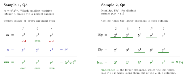
Figure 242: The two Q8s side by side, laid out as prime columns. Sample 1: a perfect square is exactly a number whose every exponent is even, so the odd columns of \(m = p^3q^2r\) are the ones needing a partner, and the smallest \(n\) that fixes them is \(pr\). Sample 2: the lcm takes the larger exponent in each column, so \(2 \cdot 3^2 \cdot 5 \cdot p \cdot q = 90pq\). The same exponent-column layout is used in gcd-lcm-and-euclidean-algorithm.
For Sample 1’s Q8 the reason fits in one line: \(mn = x^2\) \(\Leftarrow\) the prime factorisation has only even exponents. So \(n\) needs \(p^1\) and \(r^1\) in its prime factorisation, so that the exponents of \(p\) and \(r\) in the prime factorisation of \(mn\) are even. Option (A) goes separately: \(n = 0\) is impossible because \(n\) has to be a positive integer.
Sample 2’s Q8 is as short: write the two factorisations; the lcm must contain each of them and be the smallest such number. Both arguments are the Unique Factorisation Theorem doing its work — see divisibility-and-factorisation.
Part B, Q11: the same argument-validity search, twice
Both papers make Q11 a 5-mark validity question with four premises, and the model answers use the same method both times: assume every premise is true and the conclusion false, then follow what that forces. No truth table, no rules of inference — the search either closes on a contradiction, in which case the argument is valid, or it runs to completion, in which case the values it ends with are the counterexample.
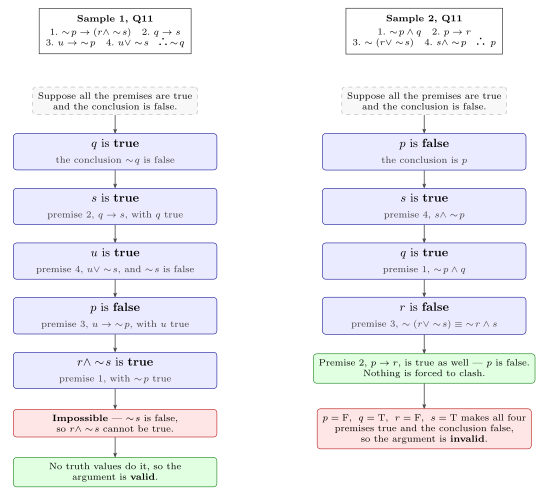
Figure 243: Part B Q11 of each paper: one search, two possible endings. Sample 1’s search closes — premise 1 demands that \(r\ \wedge \sim s\) be true, but \(\sim s\) was forced false three steps earlier, so no row can make the premises true and the conclusion false, and the argument is valid. Sample 2’s search never collides, and the four values it ends with are themselves the counterexample, so the argument is invalid. The same cascade layout is used in determining-argument-validity.
Two habits from the model answers are worth copying into your own answer.
Box every forced value as it lands — “\(q\) is true”, “\(s\) is true”, “\(u\) is true”, “\(p\) is false” — and name on each line the premise that forced it, in the form “Since premise 2 (\(q \to s\)) is true and \(q\) is true, \(s\) is true”. That is the “quality of explanation” the rubric asks for, and it costs one clause per line.
Write the verdict out in full. Sample 1 ends “So it is impossible for the argument to be invalid \(\therefore\) the argument is valid”. Sample 2 ends by restating the whole assignment — “Since truth values \(p\) false, \(q\) true, \(r\) false, \(s\) true make all premises true and the conclusion false, the argument is invalid” — because on an invalid argument the assignment is the proof, and a bare verdict has nothing behind it.
Sample 2’s premise 2 is never used to force anything; it is merely checked, at the end, and found to be satisfied automatically because \(p\) is false. Checking the unused premises is not optional — the counterexample has to make all four premises true. The full method is in determining-argument-validity, and the nine named argument forms it is an alternative to are in valid-argument-forms.
Part B, Q12: prove it or break it
Sample 1 Q12 (5 marks). Prove that for all real numbers \(q, r, s\), if \(q\) is rational, \(r\) is a non-zero rational and \(s\) is irrational, then \(q + rs\) is irrational. The model answer is a proof by contradiction, and reproducing its shape is most of the mark:
Proof (by contradiction). Suppose the statement is false. Then \(\exists q,r,s \in \mathbb{R}\) such that \(q \in \mathbb{Q}\), \(r \in \mathbb{Q}\), \(r \neq 0\) and \(s \in \overline{\mathbb{Q}}\), but \(q + rs \in \mathbb{Q}\).
Since \(q\), \(r\) and \(q+rs\) are rational, \[q = \frac{a}{b} \text{ for some } a,b \in \mathbb{Z},\ b \neq 0; \qquad r = \frac{c}{d} \text{ for some } c,d \in \mathbb{Z},\ d \neq 0,\ \text{and } c \neq 0 \text{ (since } r \neq 0);\] \[\text{and } q + rs = \frac{e}{f} \text{ for some } e,f \in \mathbb{Z},\ f \neq 0.\]
Thus \[\frac{a}{b} + \frac{c}{d}s = \frac{e}{f}, \qquad \frac{c}{d}s = \frac{e}{f} - \frac{a}{b} = \frac{eb-af}{bf}, \qquad s = \frac{d(eb-af)}{cbf}.\]
Since \(a,b,c,d,e,f \in \mathbb{Z}\), \(d(eb-af) \in \mathbb{Z}\) and \(cbf \in \mathbb{Z}\). Also \(cbf \neq 0\) since \(c \neq 0\), \(b \neq 0\) and \(f \neq 0\). Thus \(s \in \mathbb{Q}\), which is a contradiction.
\(\therefore\) The original statement is true. \(\square\)
Three details are doing the work, and each is a place marks are lost. A new letter for every new existential: six of them, \(a\) through \(f\), never reused. The non-zero conditions are tracked from the start — \(c \neq 0\) is justified on the line it is introduced, by \(r \neq 0\), and it is the only thing that makes the final division legal. And the contradiction is declared at the line it lands on — “Thus \(s \in \mathbb{Q}\), which is a contradiction” — the assumption it breaks being the \(s \in \overline{\mathbb{Q}}\) set up in the opening line. Irrational numbers are written \(\overline{\mathbb{Q}}\), the course’s notation; see rational-and-irrational-numbers and proof-techniques.
Sample 2 Q12 (5 marks) asks for a true/false verdict on two statements, with a proof or a counterexample.
(a) For all \(m,n \in \mathbb{Z}\), if \(m \mid n^2\) then \(m \mid n\). False.
Take \(m = 4\) and \(n = 2\). Then \(m,n \in \mathbb{Z}\) and \(m \mid n^2\) (since \(4 \mid 4\)) but \(m \nmid n\) (since \(4 \nmid 2\)).
That is the whole answer, and it is the course’s disproof-by-counterexample skeleton exactly: exhibit the values, check the hypothesis holds, check the conclusion fails. See divisibility-and-factorisation.
(b) For all \(n \in \mathbb{Z}^{+}\), if \(n \bmod 3 = 2\) then \(\lceil \tfrac{n}{3} \rceil = \tfrac{n+1}{3}\). True.
Proof. Let \(n \in \mathbb{Z}^{+}\) and suppose \(n \bmod 3 = 2\). Then \(n = 3k+2\) for some \(k \in \mathbb{Z}\).
Now \(\left\lceil \dfrac{n}{3} \right\rceil = \left\lceil \dfrac{3k+2}{3} \right\rceil = \left\lceil k + \dfrac{2}{3} \right\rceil = k+1\).
Also \(\dfrac{n+1}{3} = \dfrac{(3k+2)+1}{3} = \dfrac{3k+3}{3} = k+1\).
\(\therefore\ \left\lceil \dfrac{n}{3} \right\rceil = \dfrac{n+1}{3}\). \(\square\)
The move that makes it work is turning \(n \bmod 3 = 2\) into \(n = 3k+2\) immediately — the Quotient-Remainder Theorem in its usual role, converting a statement about a remainder into an algebraic form you can compute with. The two sides are then evaluated separately and shown to land on the same value, rather than being manipulated into each other; that is the same LHS/RHS discipline the course uses in induction proofs. See modular-arithmetic.
Part B, Q13: the Euclidean algorithm, and strong induction
Sample 1 Q13 runs the Euclidean algorithm and then converts the answer into an lcm. Sample 2’s Q9 runs the same algorithm on different numbers but asks something different about it, so the two are worth reading together.
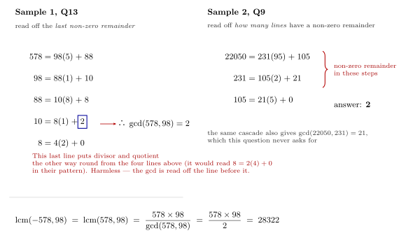
Figure 244: One algorithm, two questions. Sample 1’s Q13(a) wants the gcd, which is the last non-zero remainder — boxed at the fourth line — and part (b) then feeds it into the lcm. Sample 2’s Q9 runs the same cascade but wants only the number of lines whose remainder is non-zero, which the brace marks off. Sample 2’s cascade also yields a gcd that the question does not ask for. The last line of Sample 1’s cascade is as the solutions write it, with divisor and quotient swapped.
Part (b) is only two marks but it hides two separate facts, neither of which is on the formula page:
- \(\operatorname{lcm}(-578, 98) = \operatorname{lcm}(578, 98)\), because a number and its negative have the same multiples;
- \(\operatorname{lcm}(a,b) \cdot \gcd(a,b) = ab\), which is what makes part (a) usable in part (b) at all — and is exactly why the question says “use your answer to part (a)”.
Both are in gcd-lcm-and-euclidean-algorithm. The negative argument is the whole point of the part; it is there to catch anyone who reaches for a formula without checking what it needs.
Sample 2 Q13 (6 marks) is a strong induction: for \(a_0 = 1\), \(a_1 = 4\) and \(a_i = 2a_{i-1} + 3a_{i-2}\) for \(i \geq 2\), prove \(a_n \leq 4^n\) for every integer \(n \geq 0\).
Proof. Let \(P(n)\) be the predicate \(a_n \leq 4^n\).
Basis: Consider \(n = 0\). \(a_0 = 1\) and \(4^0 = 1\), so \(P(0)\) holds. Consider \(n=1\). \(a_1 = 4\) and \(4^1 = 4\), so \(P(1)\) holds.
Inductive hypothesis: Suppose \(k \geq 1\) is an integer and that \(P(0), P(1), \dots, P(k)\) are all true.
Consider \(n = k+1\): \[a_{k+1} = 2a_k + 3a_{k-1} \leq 2(4^k) + 3(4^{k-1}) \quad \text{by the Ind.\ Hyp.}\] \[= 4^{k-1}(2 \cdot 4 + 3) = 4^{k-1}(11) < 4^{k-1}(16) = 4^{k-1}(4^2) = 4^{k+1}.\]
\(\therefore a_{k+1} \leq 4^{k+1}\), so \(P(k+1)\) is true. Thus by the PSMI, \(a_n \leq 4^n\) for all integers \(n \geq 0\). \(\square\)
Four things this proof does deliberately:
- Two base cases, because the recurrence reaches two positions back. \(a_{k+1}\) needs both \(a_k\) and \(a_{k-1}\), so ordinary induction is not enough and one base case is not enough.
- \(k \geq 1\), not \(k \geq 0\), in the hypothesis. At \(k=0\) the step would ask for \(a_{-1}\), which does not exist. That single inequality is where a proof of this shape is most often quietly wrong.
- The inequality is used, then let go. After the first line the argument is pure algebra on \(4^{k-1}\) — factor it out, evaluate \(2\cdot 4 + 3 = 11\), and then loosen \(11\) to \(16\) because \(16 = 4^2\) is what rebuilds the power. Loosening a bound to make it fit is the move, and it is why the statement was \(\leq\) rather than \(=\) in the first place.
- The step is labelled where the hypothesis is used, on the same line — “by the Ind. Hyp.”
The principle is named “PSMI” here; the course also writes SMI, MI, PMI and the full phrase for the same two principles, so any of them is safe. See strong-induction-and-the-well-ordering-principle and mathematical-induction.
What the formula page does and does not cover
The formula-sheet is provided in the exam, so it is worth being exact about which of these questions it actually helps with. It carries the eleven named logical equivalences, the nine valid argument forms, the twelve set identities, the Quotient-Remainder Theorem, the Unique Factorisation Theorem, Schröder-Bernstein and the Binomial Theorem.
Genuinely on the page, and used: De Morgan’s and absorption (Sample 1 Q1, Q2); the Unique Factorisation Theorem behind both Q8s; the Quotient-Remainder Theorem behind Sample 1 Q7, Sample 2 Q7 and Sample 2 Q12(b); the argument forms, if you choose to do Q11 by rules of inference instead of the forced-value search.
Not on the page, and needed anyway — this is the more useful list:
- \(p \to q \equiv\ \sim p \vee q\). The definition of the conditional is not one of the eleven named equivalences, and both papers open with a Q1 that cannot be started without it.
- The contrapositive, \(p \to q \equiv\ \sim q \to\ \sim p\) (Sample 1 Q5, and the reasoning in Sample 2 Q5).
- The quantifier negation rules (Sample 1 Q3, Sample 2 Q3) — see quantified-statements.
- Necessary versus sufficient (Sample 1 Q6, Sample 2 Q5) — see conditional-statements.
- Change of variable in a summation (Sample 1 Q9).
- The well-ordering principle (Sample 1 Q10).
- The Euclidean algorithm, \(\gcd \cdot \operatorname{lcm} = ab\), and the min/max exponent rules (Sample 1 Q13; Sample 2 Q6, Q8, Q9).
- Floor and ceiling (Sample 2 Q12(b)).
- Induction in every form (Sample 2 Q13).
Nothing about proof technique is on the page either, and Part B is 15 or 16 of the marks.
Errata and wording differences
Small things, but worth knowing before you trust a line of the solutions.
Sample 2 Q4, statement II. The solutions say: “if \(x \neq 0\), take \(y = \frac{1}{x}\). Then \(\frac{x}{y} = \frac{x}{1/x} = 1 \in \mathbb{Z}\).” The conclusion is right and the verdict (statement II is true) is right, but the witness is not: \(\frac{x}{1/x} = x^2\), not \(1\). The choice that gives \(\frac{x}{y} = 1\) is \(y = x\), which is presumably what was meant — and the case split is still needed, because \(y = x\) fails at \(x = 0\), where the solutions’ second case, \(y = 1\), gives \(\frac{0}{1} = 0 \in \mathbb{Z}\).
Sample 1 Q13(a), last line. In the solutions the cascade’s first four lines are written as dividend \(=\) divisor(quotient) \(+\) remainder; the fifth is written \(8 = 4(2) + 0\), with divisor and quotient swapped. It changes nothing — the gcd is read off the line above — but the pattern breaks there. Figure 244 keeps the line as the solutions have it.
Sample 2 Q9 is worded differently in the two files. The question paper asks for “the number of steps of the algorithm in which there is a non-zero remainder”; the solutions version reads “the number of steps the algorithm in which there is a non-zero remainder when applying the quotient remainder theorem”. Same question, same answer.
Sample 2’s Q11 premise 4 is a conjunction in both files, and is worth reading twice because it is easy to see as a disjunction. Both the question paper and the solutions have \(s\ \wedge \sim p\), and the worked solution uses it as a conjunction: “Since premise 4 is true, \(s\ \wedge \sim p\) is true, so \(s\) is true”. Were it \(s\ \vee \sim p\), the search would force nothing there at all — \(\sim p\) is already true, so the disjunction would hold whatever \(s\) is.
Coverage, and what to drill
Both papers span exactly lectures 1–14 — logic, quantifiers, proof techniques, rational and irrational numbers, divisibility, modular arithmetic, the Euclidean algorithm, sequences and induction. Nothing from recursive definitions, solving recurrence relations or set theory appears in either. Every question maps onto an existing note.
The shape repeats question for question, which makes it drillable:
| Slot | Sample 1 | Sample 2 | Note |
|---|---|---|---|
| Q1–Q2 | equivalence and deduction | negation of a conditional | logical-equivalence-laws |
| Q3–Q4 | negating a quantified conditional; \(\exists\forall\) vs \(\forall\exists\) | symbolising; negating; \(\exists\forall\) vs \(\forall\exists\) | quantified-statements |
| Q5–Q6 | contrapositive; sufficient not necessary | necessary for; gcd counterexample | conditional-statements |
| Q7–Q8 | linear congruence; perfect square from a factorisation | \(\bmod\) arithmetic; lcm from factorisations | modular-arithmetic, divisibility-and-factorisation |
| Q9–Q10 | change of variable; least element | Euclidean algorithm steps; a summation-defined sequence | sequences-and-summations, strong-induction-and-the-well-ordering-principle |
| Q11 | argument validity — valid | argument validity — invalid | determining-argument-validity |
| Q12 | proof by contradiction (irrationality) | counterexample + a ceiling proof | proof-techniques |
| Q13 | Euclidean algorithm and lcm | strong induction | gcd-lcm-and-euclidean-algorithm, strong-induction-and-the-well-ordering-principle |
Part B is where the marks concentrate — 15 or 16 of 25 or 26, across three questions — and it is consistently one argument-validity question, one proof question, and one number-theory-or-induction question. Rehearse those three shapes and the layout of each; the marks for expression are handed out for exactly the habits the model answers show. More drill material is in practice-problems.
Sequences and Summations
Standard notation for sequences and summations, and the manipulations — change of variable, splitting off the last term — that every induction proof over a sum relies on. See mathematical-induction for the proofs those manipulations feed into.
Notation
A sequence is an ordered list of terms, written in any of these ways:
\[a_1, a_2, a_3, \dots \qquad (a_n)_{n \geq 0} \qquad \{a_n\}_{n=1}^{\infty}\]
These are notations for the same kind of object, not for the same sequence — note that the middle one starts at \(n = 0\) and the other two at \(n = 1\). Always read the bound.
The course uses all of these interchangeably and does not privilege one. A recursively defined sequence may be written \(\{b_n\}_{n \geq 0}\), and the braces may be dropped entirely for a bare \(a_0, a_1, a_2, \dots\). Read whichever form is in front of you; do not expect a house standard.
The subscript is the index; the bound on the index says where the sequence starts (and, if finite, where it stops). A sum over a range of the index is written
\[\sum_{n=1}^{m} a_n\]
Three ways to define a sequence
By an explicit formula that lets you calculate the value of any particular term directly.
\(a_1, a_2, a_3, \dots\) where \(a_n = 2^n - 1\), giving \(1, 3, 7, 15, 31, \dots\)
Recursively, by a rule that calculates a term from the value of one or more preceding terms.
\(\{b_n\}_{n \geq 0}\) where \(b_0 = 3\) and \(b_n = 2 \cdot b_{n-1}\) for \(n \geq 1\), giving \(3, 6, 12, 24, 48, \dots\)
The “or more” matters: the Fibonacci numbers are the standard example of a sequence whose rule reaches back two terms rather than one. A recursive definition needs both a recurrence relation and initial conditions — see recursive-definitions for what each part contributes and how to move between a recursive and an explicit definition.
In words.
For all positive integers \(n\), the sequence in which the \(n^{\text{th}}\) term is the sum of the digits of \(n^2\), giving \(1, 4, 9, 7, 7, 9, \dots\)
(Check: \(1^2 = 1\), \(2^2 = 4\), \(3^2 = 9\), \(4^2 = 16 \to 7\), \(5^2 = 25 \to 7\), \(6^2 = 36 \to 9\).)
A sequence cannot be defined by listing its first few terms
Unless you can list all of them. Initial terms never pin down a sequence — infinitely many sequences agree on any finite prefix.
What is the next term in the sequence with initial terms \(1, 4, 9, 16\)?
| Definition | Sequence |
|---|---|
| \(a_n = n^2\) | \(1, 4, 9, 16, 25, 36, \dots\) |
| \(a_n = n^2 \bmod 20\) | \(1, 4, 9, 16, 5, 16, 9, \dots\) |
Both are legitimate, and they disagree from the fifth term on. The Online Encyclopedia of Integer Sequences (https://oeis.org) returns 397 sequences for a search on \(1, 4, 9, 16\).
Working with sums
Sums over the same index range add and scale termwise:
\[\sum_{i=m}^{n} a_i \pm \sum_{i=m}^{n} b_i = \sum_{i=m}^{n} (a_i \pm b_i) \qquad\qquad \sum_{i=m}^{n} c\,a_i = c \sum_{i=m}^{n} a_i\]
The second is just factoring out the common \(c\) once the sum is written out. The general statement is on the left below and the \(c = 2\) case on the right:
\[c\,a_m + c\,a_{m+1} + \cdots + c\,a_n = c\,(a_m + \cdots + a_n) \qquad\qquad 2a_m + 2a_{m+1} + \cdots + 2a_n = 2(a_m + \cdots + a_n)\]
Note the precondition on the first identity: the two index ranges must match before the terms can be combined. Making them match is what the change of variable below is for.
Change of variable
Substituting a new index shifts the limits and rewrites the general term. To apply \(j = i + 1\) (equivalently \(i = j - 1\)) to \(\displaystyle\sum_{i=0}^{n-1} (2i + 5)\), do three things:
- lower limit: \(j = 0 + 1 = 1\)
- upper limit: \(j = (n-1) + 1 = n\)
- general term: \(2i + 5 = 2(j-1) + 5 = 2j + 3\)
\[\sum_{i=0}^{n-1} (2i+5) = \sum_{j=1}^{n} (2j+3)\]
The sum is unchanged — only its description moved. Figure 245 lays the two descriptions over the terms they describe, which is what makes that claim checkable rather than a rule to trust.
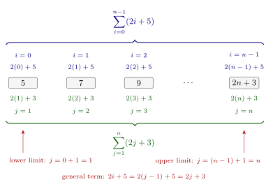
Figure 245: A change of variable relabels, it does not recompute. The boxed row is the list of numbers being added — \(5, 7, 9, \dots, 2n+3\) — and it is identical under both descriptions; only the index written above and below it changes. The three red checks are the three things the substitution has to fix, each attached to the part of the picture it governs.
Splitting off the last term
Writing a sum out and peeling the final term off is the manoeuvre used in almost every induction proof of a summation property, since it is what turns the \(P(k+1)\) side into “the \(P(k)\) side, plus one more term”:
\[\sum_{i=1}^{n+1} (3i+2) = \underbrace{(3 \cdot 1 + 2) + (3 \cdot 2 + 2) + \cdots + (3n + 2)}_{i \;=\; 1 \,\dots\, n} + \underbrace{(3(n+1) + 2)}_{i \;=\; n+1}\]
\[= \sum_{i=1}^{n} (3i+2) \; + \; (3(n+1)+2)\]
The same sum can also be split further back — peeling off the last two terms, or shifting the whole index — which is why a single sum has many equal-looking rewrites.
See also
- mathematical-induction — the proof method these manipulations serve
- recursive-definitions · solving-recurrence-relations — arithmetic and geometric sequences, and finding explicit formulas
- 2026-08-24-sequences-and-mathematical-induction — Lecture 13
- practice-problems — §16 Sequences, with full worked solutions
Sets and Set Notation
The language the rest of mathematics is written in: what a set is, the difference between belonging to one and being contained in one, and the operations that build new sets from old. See proving-set-properties for the proof methods that go with these definitions, and functions-on-general-sets for what gets built on top of them.
Writing a set down
Two ways, both used constantly:
- By listing the elements, inside braces: \(\{1,2,3\}\), \(\{a\}\), \(\{\emptyset, \{\emptyset\}\}\). An infinite list gets an ellipsis: \(\{\dots, -2, -1, 0, 1, 2, \dots\}\).
- By a defining condition — set-builder notation: \(\{n \in \mathbb{Z} \mid n \equiv 2 \;(\mathrm{mod}\; 8)\}\), read “the set of integers \(n\) such that \(n \equiv 2\) mod \(8\)”.
Both a vertical bar and a colon are used as the “such that” separator, interchangeably. \(\{n \in \mathbb{Z} \mid n \equiv 2 \;(\mathrm{mod}\; 8)\}\) and \(\{(x,y) \mid x \in \mathbb{R} \text{ and } y \in \mathbb{R}\}\) take the bar; \(f = \{(x,y) \in \mathbb{R} \times \mathbb{R} : y = 2x+1\}\) and \(f^{-1}(B) = \{x \in X : f(x) \in B\}\) take the colon. Read either as “such that”; nothing turns on which one is written.
Two conventions worth naming, because everything below relies on them: sets take capital italic letters (\(A, B, C, S, T, X, Y\)), with \(U\) reserved for the universal set, and elements take lower case (\(x\), \(y\), \(t\), \(n\)). And \(|A|\) denotes the cardinality of \(A\) — the number of elements it has (for infinite sets, where “number of elements” needs care, see [cardinality]).
“Is an element of” versus “is a subset of”
Warning. Take care with the distinction between is an element of (\(\in\)) and is a subset of (\(\subseteq\)).
This is the single most common source of error in the whole topic, and it is worth being blunt about why: the two relate different kinds of thing.
| Reads | Left-hand side is | Right-hand side is | |
|---|---|---|---|
| \(x \in A\) | \(x\) is an element of \(A\) | an object | a set |
| \(A \subseteq B\) | \(A\) is a subset of \(B\) | a set | a set |
Is \(\mathbb{Z} \in \mathbb{Q}\)? False. The elements of \(\mathbb{Q}\) are rational numbers, and \(\mathbb{Z}\) is not a number — it is a set of numbers. The true statement in the neighbourhood is \(\mathbb{Z} \subseteq \mathbb{Q}\).
The instinct behind the mistake (“but aren’t all integers rational?”) is right; it is the symbol that is wrong. “All integers are rational” is exactly the claim \(\mathbb{Z} \subseteq \mathbb{Q}\).
The same care applies one level down: a single element is not the same as the set containing that element, so \(2 \neq \{2\}\).
Worked: true or false?
| Statement | Why | ||
|---|---|---|---|
| a) | \(4 \in \{4\}\) | True | \(\{4\}\) contains \(4\) as an element |
| b) | \(4 \in \{\{4\}\}\) | False | \(\{\{4\}\}\) does not contain \(4\) as an element — it contains \(\{4\}\) as an element |
| c) | \(\{4\} \in \{2,3,4\}\) | False | \(\{2,3,4\}\) does not contain \(\{4\}\) as an element — it contains \(4\) as an element |
Each false line becomes true if you swap the symbol or the braces, which is the point of the exercise. In (c), \(\{4\} \subseteq \{2,3,4\}\) is true.
The reliable technique: write out the set’s elements and ask whether the left-hand object is literally one of the things in the list. For \(\{\{4\}\}\) that list is a single item, the set \(\{4\}\) — and \(4\) is not on it.
Subsets and proper subsets
A set \(S\) is a subset of a set \(T\), written \(S \subseteq T\), if every element in \(S\) is also in \(T\). Formally, \(\forall x\), if \(x \in S\) then \(x \in T\).
A set \(S\) is a proper subset of \(T\), written \(S \subset T\), if \(S \subseteq T\) and there is an element in \(T\) that is not in \(S\).
So \(\subset\) is \(\subseteq\) plus “and they are not equal” — exactly parallel to \(<\) against \(\leq\) for numbers.
| Holds | Fails | |
|---|---|---|
| \(\subseteq\) | \(\mathbb{Z} \subseteq \mathbb{Q}\), and \(\mathbb{Z} \subseteq \mathbb{Z}\) | |
| \(\subset\) | \(\mathbb{Z} \subset \mathbb{Q}\) | \(\mathbb{Z} \not\subset \mathbb{Z}\) |
A set is always a subset of itself and never a proper subset of itself — that single line is the whole difference between the two symbols.
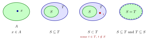
Figure 246: The four situations the symbols distinguish. An element sits inside a set; a subset is a set inside a set; a proper subset leaves something over; and equality is containment holding both ways at once. The contained set is green and the containing set pale blue, with elements as small blue dots; the red dot is the element that keeps the containment proper.
Proving one set is a subset of another
To prove \(S \subseteq T\), consider an arbitrary element of \(S\) and show it is also in \(T\). That is: suppose \(x \in S\), and prove \(x \in T\).
This is the element method, and it is used so heavily that proving-set-properties treats it in full. The word doing the work is “arbitrary” — you may assume nothing about \(x\) beyond membership of \(S\), which is what makes the one argument cover every element at once.
Worked. Let \(D = \{n \in \mathbb{Z} \mid n \equiv 2 \;(\mathrm{mod}\; 8)\}\) and let \(E\) be the set of even integers, i.e. \(E = \{n \in \mathbb{Z} \mid n \equiv 0 \;(\mathrm{mod}\; 2)\}\). Prove \(D \subseteq E\).
Proof. Let \(x \in D\). Then \(x \equiv 2 \;(\mathrm{mod}\; 8)\), so there exists \(k \in \mathbb{Z}\) such that \[x = 8k + 2 = 2(4k + 1) + 0\] Since \(4k + 1 \in \mathbb{Z}\), we have \(x \equiv 0 \;(\mathrm{mod}\; 2)\), and therefore \(x \in E\). Thus \(D \subseteq E\). \(\blacksquare\)
Rewriting \(8k+2\) as \(2(4k+1)\) is the entire proof — see modular-arithmetic for the definition being applied.
Is \(D \subset E\)? Yes. We have \(D \subseteq E\), and \(4 \in E\) while \(4 \notin D\) (since \(4 \not\equiv 2 \bmod 8\)), so the containment is proper. Note that upgrading \(\subseteq\) to \(\subset\) needs one witness, not a general argument.
When are two sets equal?
For sets \(S\) and \(T\), \(S = T\) means \(\forall x\), \(x \in S\) if and only if \(x \in T\).
Recall that \(S \subseteq T\) means \(\forall x\), if \(x \in S\) then \(x \in T\). Since \(p \leftrightarrow q \equiv (p \rightarrow q) \land (q \rightarrow p)\), it follows that
\[S = T \quad\text{is logically equivalent to}\quad (S \subseteq T) \land (T \subseteq S)\]
So to prove two sets are equal, do two separate proofs:
- Suppose \(x \in S\), and prove \(x \in T\). This shows \(S \subseteq T\).
- Suppose \(x \in T\), and prove \(x \in S\). This shows \(T \subseteq S\).
Together these give \(S = T\). This is not a convention but a consequence — the double containment argument is just the biconditional law of logical-equivalence-laws read through the definition of \(\subseteq\), which is why “prove both directions” is never optional.
The empty set
\(\emptyset = \{\;\}\) — the set with no elements.
Why is \(\emptyset \subseteq A\) for every set \(A\)? Because “\(\forall x\), if \(x \in \emptyset\) then \(x \in A\)” is true for every set \(A\). The hypothesis \(x \in \emptyset\) is never satisfied, and a conditional with a false hypothesis is true — so the statement holds vacuously. See conditional-statements for that truth-table row, which is doing all the work here.
Do not confuse this with \(\emptyset \in A\). Some sets do contain the empty set as an element; many do not. \(\emptyset \subseteq A\) is a theorem about every set; \(\emptyset \in A\) is a claim about one particular set that usually fails.
Why is \(A \subseteq A\) for every set \(A\)? Because “\(\forall x\), if \(x \in A\) then \(x \in A\)” is true for every set \(A\) — this one for the opposite reason, that the conclusion simply restates the hypothesis.
There is only one empty set
Lemma. There is only one empty set.
Proof (by contradiction). Suppose \(\emptyset_1\) and \(\emptyset_2\) are distinct sets each having no elements, so \(\emptyset_1 \neq \emptyset_2\). Since \(\emptyset_1\) has no elements, it is a subset of \(\emptyset_2\); that is, \(\emptyset_1 \subseteq \emptyset_2\). Also, since \(\emptyset_2\) has no elements, \(\emptyset_2 \subseteq \emptyset_1\). Thus \(\emptyset_1 = \emptyset_2\) by definition of set equality — contradicting the supposition. \(\blacksquare\)
This is why we say the empty set and write a single symbol for it. The proof is a neat demonstration of the double-containment criterion doing real work: both containments come free from vacuous truth, and equality falls out.
Unions and intersections
\[A \cup B = \{x \mid x \in A \text{ or } x \in B\} \qquad\qquad A \cap B = \{x \mid x \in A \text{ and } x \in B\}\]
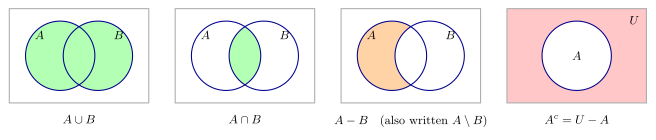
Figure 247: The four operations as shaded regions. Union takes everything in either circle, intersection only the overlap, difference removes B from A, and the complement is everything in the universe outside A — which is why a complement is only meaningful once the universe U is fixed. The enclosing rectangle is that universe.
Worked. Let \(A_1 = \{1,2,3\}\), \(A_2 = \{1,2,4\}\) and \(A_3 = \{3,4,5\}\).
\[A_1 \cup A_2 = \{1,2,3,4\} \qquad A_1 \cap A_2 = \{1,2\} \qquad A_1 \cap A_3 = \{3\} \qquad A_2 \cap A_3 = \{4\}\]
Indexed over all three:
\[\bigcup_{i=1}^{3} A_i = A_1 \cup A_2 \cup A_3 = \{1,2,3,4,5\} \qquad\qquad \bigcap_{i=1}^{3} A_i = (A_1 \cap A_2) \cap A_3 = \{1,2\} \cap \{3,4,5\} = \emptyset\]
Worth noticing: the three sets intersect pairwise in a non-empty set every time, and yet the triple intersection is empty. Pairwise overlap does not survive to the whole family, so an indexed intersection has to be computed, not inferred.
Indexed families
\[\bigcup_{i \in I} A_i = \{x \mid x \in A_i \text{ for \textbf{at least one} } i \in I\} \qquad \bigcap_{i \in I} A_i = \{x \mid x \in A_i \text{ for \textbf{every} } i \in I\}\]
These extend to infinite index sets unchanged, which is where they earn their keep.
Worked, over \(i = 0, 1, 2, \dots\):
\[\bigcup_{i=0}^{\infty} \{i, -i\} = \{0\} \cup \{1,-1\} \cup \{2,-2\} \cup \cdots = \{\dots, -2, -1, 0, 1, 2, \dots\} = \mathbb{Z}\]
\[\bigcap_{i=0}^{\infty} [-i,\, i] = \{0\}\]
recalling the interval notation \([a,b] = \{x \in \mathbb{R} \mid a \leq x \leq b\}\).
The intersection is the interesting one. The intervals grow as \(i\) increases, so the intersection is pinned by the smallest of them, the \(i = 0\) term \([0,0] = \{0\}\). Every larger interval contains \(0\), so nothing is lost, and nothing else survives.
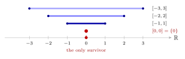
Figure 248: An intersection over an increasing family is decided by its smallest member. Each interval contains the one below it, so the only real number lying in all of them is the single point the innermost interval contains. The intervals sit above the number line, with a filled dot at each closed endpoint.
Set difference and complement
\[A - B = \{x \mid x \in A \text{ and } x \notin B\}\]
Both are drawn in Figure 247 above.
The backslash and the minus sign mean the same thing: \(A - B\) can equally be written \(A \setminus B\). Different textbooks pick different ones; there is no distinction to learn.
The complement \(A^{c}\) is the set difference from the universal set \(U\) under discussion: \(A^{c} = U - A\). It is only meaningful once \(U\) is fixed, so a complement always sits inside a stated universe.
The power set
\(\mathcal{P}(A)\) is the set of all subsets of \(A\).
Worked. Let \(S = \{1,2,3\}\). Then
\[\mathcal{P}(S) = \big\{\, \emptyset,\; \{1\},\; \{2\},\; \{3\},\; \{1,2\},\; \{1,3\},\; \{2,3\},\; \{1,2,3\} \,\big\}\]
Note that the elements of \(\mathcal{P}(S)\) are sets, which resets the \(\in\) / \(\subseteq\) trap one level up:
| Statement | Why | |
|---|---|---|
| \(\{1,2\} \in \mathcal{P}(S)\) | True | \(\{1,2\}\) is one of the eight things listed |
| \(\{1,2\} \subseteq \mathcal{P}(S)\) | False | that would need \(1\) and \(2\) themselves to be elements of \(\mathcal{P}(S)\), i.e. to be subsets of \(S\) — and they are numbers, not sets |
| \(\big\{\{1,2\}\big\} \subseteq \mathcal{P}(S)\) | True | the one element it has, \(\{1,2\}\), is in \(\mathcal{P}(S)\) |
Also worth recording as a standing fact: since \(\emptyset \subseteq A\) for every set \(A\), it follows that \(\emptyset \in \mathcal{P}(A)\) for every set \(A\). Every power set is non-empty, including \(\mathcal{P}(\emptyset)\).
Fact. If \(T\) is a finite set with \(n\) elements, then \(|\mathcal{P}(T)| = 2^{n}\).
The finiteness matters — the count is meaningless otherwise. The \(2^n\) comes from building a subset by making \(n\) independent in/out choices. Sorting the same subsets by size instead gives \(\binom{n}{0} + \binom{n}{1} + \cdots + \binom{n}{n} = 2^n\) (binomial-coefficients).
Worked: is \(\{1, 3, -1\} \subset \mathcal{P}(\mathbb{Z})\)?
False, and the reasoning is the \(\in\)/\(\subseteq\) distinction again, run carefully:
- \(1, 3, -1 \in \mathbb{Z}\), so \(\{1,3,-1\} \subseteq \mathbb{Z}\).
- Therefore \(\{1,3,-1\} \in \mathcal{P}(\mathbb{Z})\) — it is one of the subsets of \(\mathbb{Z}\), hence an element of the power set.
- So \(\{1,3,-1\} \not\subset \mathcal{P}(\mathbb{Z})\): for that, its elements \(1\), \(3\) and \(-1\) would have to be elements of \(\mathcal{P}(\mathbb{Z})\), i.e. subsets of \(\mathbb{Z}\) — and they are integers, not sets.
The statement is off by exactly one level, which is the characteristic failure mode with power sets.
Worked: power sets of power sets
Building up from the empty set, with the \(2^n\) fact as a running check:
| Value | \(|\,\cdot\,|\) of the input | Check | |
|---|---|---|---|
| \(\mathcal{P}(\{a\})\) | \(\big\{\emptyset,\; \{a\}\big\}\) | \(|\{a\}| = 1\) | \(2^1 = 2\) \(\checkmark\) |
| \(\mathcal{P}(\emptyset)\) | \(\big\{\emptyset\big\}\) | \(|\emptyset| = 0\) | \(2^0 = 1\) \(\checkmark\) |
| \(\mathcal{P}(\mathcal{P}(\emptyset)) = \mathcal{P}(\{\emptyset\})\) | \(\big\{\emptyset,\; \{\emptyset\}\big\}\) | \(|\{\emptyset\}| = 1\) | \(2^1 = 2\) \(\checkmark\) |
| \(\mathcal{P}(\mathcal{P}(\mathcal{P}(\emptyset))) = \mathcal{P}\big(\{\emptyset, \{\emptyset\}\}\big)\) | \(\big\{\emptyset,\; \{\emptyset\},\; \{\{\emptyset\}\},\; \{\emptyset, \{\emptyset\}\}\big\}\) | \(\big|\{\emptyset,\{\emptyset\}\}\big| = 2\) | \(2^2 = 4\) \(\checkmark\) |
\(\mathcal{P}(\emptyset) = \{\emptyset\}\) is the line to get right: the empty set has exactly one subset — itself — so its power set has one element and is not empty. Counting the elements at each stage and checking against \(2^n\) is the cheapest way to catch a dropped or duplicated brace.
Cartesian products
\[A \times B = \{(a,b) \mid a \in A \text{ and } b \in B\}\]
the set of ordered pairs with first coordinate from \(A\) and second from \(B\).
Worked. \(A_1 = \{1,2\}\), \(A_2 = \{3,4,5\}\), \(A_3 = \{6\}\).
\[A_1 \times A_2 = \{(1,3), (1,4), (1,5), (2,3), (2,4), (2,5)\}\]
\[A_1 \times A_2 \times A_3 = \{(1,3,6), (1,4,6), (1,5,6), (2,3,6), (2,4,6), (2,5,6)\}\]
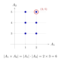
Figure 249: A Cartesian product laid out as a grid: one row per element of the first set, one column per element of the second, one ordered pair at every crossing. The rectangular shape is the counting fact — the number of pairs is the product of the two sizes.
Worked. Let \(S = \{a,b,c\}\) and \(T = \{c,d\}\).
- \((d,c) \notin S \times T\), since \(d \notin S\) — the order matters, and \(d\) is disqualified as a first coordinate.
- \((c,d) \in S \times T\), since \(c \in S\) and \(d \in T\).
- \(S \times T\) contains \(3 \times 2 = 6\) elements.
The familiar case is \(\mathbb{R} \times \mathbb{R} = \{(x,y) \mid x \in \mathbb{R} \text{ and } y \in \mathbb{R}\}\), usually written \(\mathbb{R}^2\) — the plane is a Cartesian product, which is where the name comes from.
Two facts:
- If \(A = \emptyset\) or \(B = \emptyset\) then \(A \times B = \emptyset\) — there is no way to choose a coordinate from an empty set.
- For finite sets, \(|A_1 \times A_2 \times \cdots \times A_n| = |A_1| \cdot |A_2| \cdots |A_n|\).
Notation clash to be aware of. \((a,b)\) can mean an ordered pair, and \((a,b)\) can also mean an open interval — the real numbers \(x\) with \(a < x < b\). Nothing in the symbols distinguishes them; only the context does.
Partitions
A finite or infinite collection of non-empty sets \(\{A_1, A_2, A_3, \dots\}\) is a partition of a set \(A\) if and only if \[A = A_1 \cup A_2 \cup A_3 \cup \cdots \qquad\text{and}\qquad A_i \cap A_j = \emptyset \text{ for each } i, j \geq 1,\; i \neq j\]
Three conditions, all of which are checkable and all of which get tested: the pieces are non-empty, they cover \(A\), and they are pairwise disjoint.
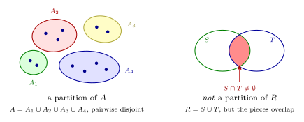
Figure 250: A partition cuts a set into non-empty pieces that cover it with no overlap — every element lands in exactly one piece. Failing any one of the three conditions is enough to disqualify a collection. On the left is a partition: separate closed curves, one per piece, each holding its elements as dots. On the right, two pieces share an element, so the collection is not a partition.
Examples over \(\mathbb{Z}\):
- \(\{E, O\}\), where \(E\) is the even integers and \(O\) the odd integers, is a partition of \(\mathbb{Z}\).
- \(\big\{\{0\},\; \mathbb{Z}^{+},\; \mathbb{Z}^{-}\big\}\) is another partition of \(\mathbb{Z}\) — a set can be partitioned in many ways.
Worked: a collection that fails
Let \(S = \{x \in \mathbb{Z} \mid x \equiv 1 \;(\mathrm{mod}\; 3)\}\), let \(T = \{x \in \mathbb{Z} \mid x \equiv 2 \;(\mathrm{mod}\; 4)\}\), and let \(R = S \cup T\). Is \(\{S, T\}\) a partition of \(R\)?
No. The covering condition holds by construction — \(R = S \cup T\) is how \(R\) was defined. But disjointness fails:
\[10 = 3(3) + 1 \;\Rightarrow\; 10 \equiv 1 \;(\mathrm{mod}\; 3) \;\Rightarrow\; 10 \in S\] \[10 = 4(2) + 2 \;\Rightarrow\; 10 \equiv 2 \;(\mathrm{mod}\; 4) \;\Rightarrow\; 10 \in T\]
so \(10 \in S \cap T\) and \(S \cap T \neq \emptyset\). Therefore \(\{S,T\}\) is not a partition of \(R\).
A single witness settles it — disjointness is a universal claim, so one counterexample is a complete disproof.
Worked: two partitions of \(\mathbb{Z} \times \mathbb{Z}\)
Any rule that sorts every pair into exactly one bucket works. Two independent ways:
By the sign of the first coordinate. \[P = \{(a,b) \in \mathbb{Z} \times \mathbb{Z} \mid a \geq 0\} \qquad N = \{(a,b) \in \mathbb{Z} \times \mathbb{Z} \mid a < 0\}\] \(\{N, P\}\) is a partition of \(\mathbb{Z} \times \mathbb{Z}\) — every integer \(a\) is either \(\geq 0\) or \(< 0\), never both.
By the parity of the second coordinate. \[E = \{(a,b) \in \mathbb{Z} \times \mathbb{Z} \mid b \equiv 0 \;(\mathrm{mod}\; 2)\} \qquad O = \{(a,b) \in \mathbb{Z} \times \mathbb{Z} \mid b \equiv 1 \;(\mathrm{mod}\; 2)\}\] \(\{E, O\}\) is another partition of \(\mathbb{Z} \times \mathbb{Z}\).
The recipe generalises: take any property that every element either has or lacks, and the two resulting sets partition the whole — provided neither comes out empty. That connection is made exact by equivalence relations: every partition is the set of classes of one, and the other way round (equivalence-classes-and-partitions).
See also
- proving-set-properties — the element method, the set identities, and proofs about these operations
- functions-on-general-sets — functions defined as subsets of a Cartesian product
- equivalence-classes-and-partitions — partitions as the classes of an equivalence relation
- modular-arithmetic — the congruence sets used throughout the worked examples
- counting-principles · counting-selections — \(|A \times B| = |A| \times |B|\) as the multiplication rule, and \(\binom{n}{r}\), the number of \(r\)-element subsets of an \(n\)-element set
- inclusion-exclusion · [probability] — the size of a union of sets that overlap, with De Morgan’s law for “neither”, and events as subsets of a sample space
- pigeonhole-principle — a partition as the set of pigeonholes
- conditional-statements · logical-equivalence-laws — vacuous truth, and the biconditional behind set equality
- 2026-09-03-set-theory-definitions — Lecture 17
- practice-problems — §21 Set Theory Definitions, with full worked solutions
- practice-problems — §22 More Definitions and Examples of Sets
Solving Recurrence Relations
recursive-definitions builds a sequence out of its own earlier terms. This note goes the other way: given a recursive definition, find an explicit formula for the \(n^{\text{th}}\) term, and prove the formula is right. See mathematical-induction and strong-induction-and-the-well-ordering-principle for the proof machinery the second method leans on.
Two ways of writing the same sequence
Every sequence here can be described twice over, and the two descriptions are worth naming precisely because the whole topic is moving between them:
| Shape | What it lets you do | |
|---|---|---|
| Recurrence relation | \(a_k = \dots a_{k-1} \dots\) | get the next term from the ones before it |
| Explicit formula | \(a_n = \dots n \dots\) | get any term without computing the others |
The subscript is the tell. A rule written in \(k\) that mentions \(a_{k-1}\) is a recurrence relation; a rule written in \(n\) that mentions only \(n\) is an explicit formula.
Arithmetic and geometric sequences
The two standard families, in both forms — for a sequence \(a_0, a_1, a_2, \dots\):
| Recurrence relation | Explicit formula | |
|---|---|---|
| Arithmetic | \(a_k = a_{k-1} + d\) for integers \(k \geq 1\) | \(a_n = a_0 + dn\) for integers \(n \geq 0\) |
| Geometric | \(a_k = r \cdot a_{k-1}\) for integers \(k \geq 1\) | \(a_n = a_0 \cdot r^{\,n}\) for integers \(n \geq 0\) |
\(d\) is the common difference and \(r\) the common ratio. Both explicit formulas are the recurrence applied \(n\) times from \(a_0\), which is why the index of the seed and the exponent agree: \(a_n\) is \(n\) steps away from \(a_0\).
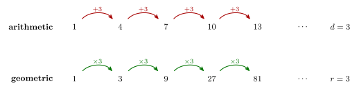
Figure 251: The two families as operations between consecutive terms. Arithmetic adds the same \(d\) at every step; geometric multiplies by the same \(r\). Reading a sequence means testing the gaps: constant differences means arithmetic, constant ratios means geometric.
Worked the other way, from terms to a formula: \(2, 6, 18, 54, \dots\) multiplies by \(3\) each step, so \(r = 3\); the seed is \(a_0 = 2\); hence \(a_n = 2 \cdot 3^{\,n}\).
Telling them apart
Deciding which family a run of terms belongs to is a matter of computing the gaps both ways, not of eyeballing.
Do \(\tfrac{5}{8}, \tfrac{5}{2}, 10\) sit in an arithmetic sequence, a geometric one, both, or neither?
Put everything over the same denominator — \(\tfrac{5}{8}, \tfrac{20}{8}, \tfrac{80}{8}\) — and both tests become easy:
| Test | First gap | Second gap | Verdict |
|---|---|---|---|
| Differences | \(\tfrac{20}{8} - \tfrac{5}{8} = \tfrac{15}{8}\) | \(\tfrac{80}{8} - \tfrac{20}{8} = \tfrac{60}{8}\) | not equal — not arithmetic |
| Ratios | \(\tfrac{5}{2} \div \tfrac{5}{8} = 4\) | \(10 \div \tfrac{5}{2} = 4\) | equal — geometric, \(r = 4\) |
So the answer is geometric only. The common trap is “both”: a sequence that passes the ratio test has no obligation to pass the difference test, and here it plainly fails it.
Do \(2, 2, 2\)? This one is both. The differences are all \(0\), so it is arithmetic with \(d = 0\); the ratios are all \(1\), so it is geometric with \(r = 1\). It is a constant sequence \(a_n = c\), which is what you get from \(d = 0\) on one side and \(r = 1\) on the other. The constant sequences are the whole of the overlap and not merely examples of it: \(a_0 + dn\) and \(a_0 r^{\,n}\) can agree for every \(n\) only if \(d = 0\), and then both are constant.
One convention worth knowing: many texts require \(a_0 \neq 0\) and \(r \neq 0\) for a geometric sequence, which excludes the all-zeros sequence \(0, 0, 0, \dots\) — every \(r\) satisfies \(0 = r \cdot 0\), so the common ratio would not be determined. \(2, 2, 2\) is unaffected.
From a recursive definition to an explicit formula
The workflow is always the same three steps:
- Calculate the first few terms from the recursive definition.
- Guess an explicit formula that fits them.
- Prove the guess is correct.
Step 3 is not optional, and it is the whole difficulty: any finite run of terms is consistent with infinitely many formulas (see sequences-and-summations on why listing terms never defines a sequence). Two methods are available.
| Method 1 | Method 2 | |
|---|---|---|
| What you show | the formula gives the right initial conditions, and satisfies the recurrence relation | the formula holds for every \(n\), by (strong) mathematical induction |
| In a word | quicker | rigorous |
Why Method 1 is a proof and not just a check
Method 1 can look like it is only testing a couple of cases, so it is worth seeing why it settles the matter. A recursive definition determines its sequence uniquely: the initial conditions fix the first terms, and the recurrence relation then forces every later one. So if your formula reproduces the initial conditions and obeys the same recurrence, it generates the same sequence term by term — there is nowhere for the two to diverge. That is the entire content of Method 1, and it is why the two checks it makes are exactly the two halves of the definition.
Method 2 makes that argument explicitly rather than appealing to it, which is why it is the more rigorous of the two and the one to use when a question says “prove by induction”.
The Method 1 template
Given a guess \(a_n = f(n)\):
- Initial conditions. Substitute the seed index into \(f\) and check it returns the stated value. One check per initial condition.
- Recurrence relation. Write down both sides separately, substituting the guess wherever an earlier term appears, and show they agree:
\[\text{LHS} = a_k = f(k) \qquad\qquad \text{RHS} = \big(\text{the recurrence, with } f(k-1),\, f(k-2),\, \dots \text{ substituted}\big)\]
Set the two sides out under the labels LHS and RHS and meet in the middle. That keeps you from the circularity of starting with what you are trying to prove.
The Method 2 template
Take \(P(n)\) to be the predicate \(a_n = f(n)\) and run an induction. Which induction depends on the recurrence:
| The recurrence reaches back | Use | Basis step needs |
|---|---|---|
| one term (\(a_{k-1}\)) | ordinary induction (MI) | one base case |
| two or more terms (\(a_{k-1}, a_{k-2}, \dots\)) | strong induction (SMI) | one base case per initial condition |
The rule is not arbitrary: to get \(P(k+1)\) from a recurrence mentioning \(a_{k-1}\), you need \(P(k-1)\) as well as \(P(k)\), and only the strong hypothesis hands you both.
Worked examples
A recurrence reaching back one term
\(c_1 = 1\) and \(c_k = c_{k-1} + 2^k\) for each integer \(k \geq 2\). Is this the sequence \(c_n = 2^{\,n+1} - 3\) for each integer \(n \geq 1\)?
Method 1.
Initial condition \((n = 1)\): \(\;c_1 = 2^{1+1} - 3 = 4 - 3 = 1\;\) ✓
Recurrence relation:
\[\text{LHS} = c_k = 2^{k+1} - 3\] \[\text{RHS} = c_{k-1} + 2^k = \big(2^{(k-1)+1} - 3\big) + 2^k = 2^k + 2^k - 3 = 2\big(2^k\big) - 3 = 2^{k+1} - 3\]
LHS \(=\) RHS, so the formula satisfies the recurrence. The statement is true.
Method 2. Let \(P(n)\) be the predicate \(c_n = 2^{\,n+1} - 3\).
Basis step. \(c_1 = 1\) by the recursive definition, and \(2^{1+1} - 3 = 4 - 3 = 1\), so \(P(1)\) is true.
Inductive hypothesis. Suppose \(P(k)\) is true for some integer \(k \geq 1\), i.e. \(c_k = 2^{k+1} - 3\). Then
\[c_{k+1} = c_k + 2^{k+1} = \big(2^{k+1} - 3\big) + 2^{k+1} = 2\big(2^{k+1}\big) - 3 = 2^{k+2} - 3\]
so \(P(k+1)\) is true. Hence by mathematical induction \(c_n = 2^{\,n+1} - 3\) for each integer \(n \geq 1\). \(\blacksquare\)
Note the shape of the inductive step: substitute the recurrence, then the hypothesis, then collect. The two \(2^{k+1}\) terms combining into \(2^{k+2}\) is the only real move.
A recurrence reaching back two terms
\(b_0 = 0\), \(b_1 = 1\) and \(b_k = \tfrac{1}{2}\big(b_{k-1} + b_{k-2} + 1\big) + 3(k-1)\) for each integer \(k \geq 2\).
Calculating terms. Each one uses the two before it:
\[b_2 = \tfrac{1}{2}(1 + 0 + 1) + 3(1) = 1 + 3 = 4\] \[b_3 = \tfrac{1}{2}(4 + 1 + 1) + 3(2) = 3 + 6 = 9\] \[b_4 = \tfrac{1}{2}(9 + 4 + 1) + 3(3) = 7 + 9 = 16\]
giving \(0, 1, 4, 9, 16, \dots\) — guess \(b_n = n^2\) for all integers \(n \geq 0\).
Method 1.
Initial conditions: \(b_0 = 0^2 = 0\) ✓ and \(b_1 = 1^2 = 1\) ✓ — two conditions, two checks.
Recurrence relation:
\[\text{LHS} = b_k = k^2\]
\[\begin{aligned} \text{RHS} &= \tfrac{1}{2}\big((k-1)^2 + (k-2)^2 + 1\big) + 3(k-1) \\ &= \tfrac{1}{2}\big(k^2 - 2k + 1 + k^2 - 4k + 4 + 1\big) + 3k - 3 \\ &= \tfrac{1}{2}\big(2k^2 - 6k + 6\big) + 3k - 3 \\ &= \big(k^2 - 3k + 3\big) + 3k - 3 \\ &= k^2 \end{aligned}\]
LHS \(=\) RHS, so the explicit formula satisfies the recurrence relation.
Method 2, by strong induction — two terms back, so SMI and two base cases.
Basis step. \(b_0 = 0\) and \(0^2 = 0\), so \(P(0)\) holds; \(b_1 = 1\) and \(1^2 = 1\), so \(P(1)\) holds.
Inductive hypothesis. Suppose \(k \geq 1\) is an integer and \(P(0), P(1), \dots, P(k)\) are each true. Then
\[\begin{aligned} b_{k+1} &= \tfrac{1}{2}\big(b_k + b_{k-1} + 1\big) + 3\big((k+1) - 1\big) \\ &= \tfrac{1}{2}\big(k^2 + (k-1)^2 + 1\big) + 3k \\ &= \tfrac{1}{2}\big(k^2 + k^2 - 2k + 1 + 1\big) + 3k \\ &= \tfrac{1}{2}\big(2k^2 - 2k + 2\big) + 3k \\ &= k^2 - k + 1 + 3k \\ &= k^2 + 2k + 1 = (k+1)^2 \end{aligned}\]
so \(P(k+1)\) is true, and by SMI \(b_n = n^2\) for each integer \(n \geq 0\). \(\blacksquare\)
The hypothesis is used twice here — once for \(b_k\) and once for \(b_{k-1}\) — which is precisely what ordinary induction could not have supplied.
The same sequence, a different recursive definition
Find a different recursive definition of \(\{b_n\}_{n \geq 0}\).
Once the explicit formula is known this is easy, and it makes the point that a sequence does not have one recursive definition. Look for a one-term recurrence \(b_n = b_{n-1} + p\) and solve for the step \(p\):
\[n^2 = (n-1)^2 + p \;\implies\; p = n^2 - (n-1)^2 = 2n - 1\]
so \(b_0 = 0\) and \(b_n = b_{n-1} + (2n-1)\) for all integers \(n \geq 1\) defines the same sequence — the familiar fact that the squares are the running totals of the odd numbers. Note it needs only one initial condition where the original needed two.
A recurrence that is not a polynomial
\(d_0 = 1\) and \(d_k = \dfrac{d_{k-1}}{1 + d_{k-1}}\) for each integer \(k \geq 1\).
Calculating terms. The useful move is multiplying by a disguised \(1\) to clear the fraction inside the fraction:
\[d_1 = \frac{1}{1+1} = \frac{1}{2}\] \[d_2 = \frac{\tfrac{1}{2}}{1 + \tfrac{1}{2}} \cdot \frac{2}{2} = \frac{1}{2 + 1} = \frac{1}{3} \qquad d_3 = \frac{\tfrac{1}{3}}{1 + \tfrac{1}{3}} \cdot \frac{3}{3} = \frac{1}{3 + 1} = \frac{1}{4}\]
giving \(1, \tfrac12, \tfrac13, \tfrac14, \dots\) — guess \(d_n = \dfrac{1}{n+1}\) for all integers \(n \geq 0\).
That \(\times \tfrac{k}{k}\) trick is worth keeping: multiplying numerator and denominator by the denominator of the inner fraction turns a compound fraction into a simple one in one step, with no common-denominator bookkeeping.
Method 1.
Initial condition \((d_0 = 1)\): \(\;d_0 = \dfrac{1}{0+1} = 1\;\) ✓
Recurrence relation:
\[\text{LHS} = d_k = \frac{1}{k+1} \qquad \text{RHS} = \frac{d_{k-1}}{1 + d_{k-1}} = \frac{\tfrac{1}{k}}{1 + \tfrac{1}{k}} \cdot \frac{k}{k} = \frac{1}{k+1}\]
LHS \(=\) RHS. ✓
Method 2, by ordinary induction — the recurrence reaches back one term, so MI and one base case.
Basis step. \(d_0 = 1\) from the definition and \(\tfrac{1}{0+1} = 1\), so \(P(0)\) is true.
Inductive hypothesis. Suppose \(P(k)\) is true for some integer \(k \geq 0\). Then
\[d_{k+1} = \frac{d_k}{1 + d_k} = \frac{1/(k+1)}{1 + 1/(k+1)} = \frac{1/(k+1)}{(k+2)/(k+1)} = \frac{1}{k+1} \cdot \frac{k+1}{k+2} = \frac{1}{k+2}\]
which is \(\tfrac{1}{(k+1)+1}\), so \(P(k+1)\) is true. By MI, \(d_n = \dfrac{1}{n+1}\) for each integer \(n \geq 0\). \(\blacksquare\)
The Tower of Hanoi
Given a tower of 8 discs of decreasing size on one of three pegs, transfer the whole tower to another peg, subject to two rules: move only one disc at a time, and never move a larger disc onto a smaller one. Is there a solution, and if so what is the fewest number of moves?
This is the standard example of a recurrence that comes out of an argument rather than out of a formula. For \(n \geq 1\) let \(m_n\) be the minimum number of moves needed to transfer a tower of \(n\) discs from one peg to another.
Small cases first: \(m_1 = 1\) — move the single disc. \(m_2 = 3\) — small disc to the spare peg, large disc to the target, small disc back on top.
The general case is the recursive insight:

Figure 252: Why the recurrence doubles and adds one. Each box is one position of the three pegs, with discs as bars, the widest at the bottom, and the moves run left to right. To move \(k\) discs you must at some point move the largest, and it can only go onto an empty peg — so the other \(k-1\) discs have to be parked on the spare peg first, then brought back on top afterwards. Two sub-transfers of \(k-1\) discs, plus the single move of the largest. The \(k-1\) smaller discs are drawn as a stack of three for legibility; nothing in the argument depends on how many there are.
Reading the picture off as arithmetic gives, for example, \(m_4 = m_3 + 1 + m_3\), and in general
\[m_1 = 1 \qquad\text{and}\qquad m_k = 2m_{k-1} + 1 \;\text{ for all integers } k \geq 2\]
The explicit formula. The textbook (p. 310 in the 4th edition, p. 346 in the 5th) guesses \(m_n = 2^n - 1\) for all integers \(n \geq 1\). By Method 1:
Initial condition \((m_1 = 1)\): \(\;m_1 = 2^1 - 1 = 2 - 1 = 1\;\) ✓
Recurrence relation:
\[\text{LHS} = m_k = 2^k - 1\] \[\text{RHS} = 2m_{k-1} + 1 = 2\big(2^{\,k-1} - 1\big) + 1 = 2 \cdot 2^{\,k-1} - 2 + 1 = 2^k - 1\]
LHS \(=\) RHS, so the guess is correct. The textbook proves the same result by mathematical induction — either method is acceptable.
So the eight-disc tower takes \(2^8 - 1 = 255\) moves, and the answer to “is there a solution?” is yes, constructively, because the recursion is the algorithm.
See also
- recursive-definitions — the other direction, and recursively defined sets
- sequences-and-summations — sequence notation, and why initial terms never define a sequence
- mathematical-induction · strong-induction-and-the-well-ordering-principle — Method 2’s machinery
- 2026-08-31-solving-recurrence-relations — Lecture 16
- practice-problems — §20 Solving Recurrence Relations, with full worked solutions
Strong Induction and the Well-Ordering Principle
Strong mathematical induction, the well-ordering principle for the integers, and the sense in which these two and ordinary induction are all the same tool. See mathematical-induction for ordinary induction and the four-step proof template both methods share.
Strong mathematical induction
Let \(P(n)\) be a predicate written in terms of some integer \(n\). The difference from ordinary induction is entirely in what the inductive step is allowed to assume: every earlier case, not just the immediately preceding one — and, to pay for that, a basis step that establishes several cases rather than one.
| Ordinary induction (MI) | Strong induction (SMI) | |
|---|---|---|
| Basis step | \(P(2)\) | \(P(2) \wedge P(3) \wedge P(4)\) |
| Inductive step | \(\forall k \in \mathbb{Z}\) with \(k \geq 2\), if \(P(k)\) then \(P(k+1)\) | \(\forall k \in \mathbb{Z}\) with \(k \geq 4\), if \(P(2) \wedge P(3) \wedge \cdots \wedge P(k)\) then \(P(k+1)\) |
| Conclusion | \(P(n)\) for each integer \(n \geq 2\) | \(P(n)\) for each integer \(n \geq 2\) |
Both reach the same conclusion by the same kind of chain. For MI, \(P(5)\) follows from \(P(2)\) by three applications of the implication; for SMI with the basis above, \(P(6)\) follows in two.
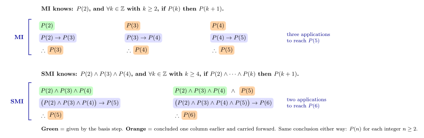
Figure 253: Mathematical induction and strong mathematical induction as chains of inferences. Each column is an argument — premises stacked, conclusion prefixed by ∴, no rule line. MI climbs one rung at a time from a single base case; SMI starts from three base cases and each step may lean on everything established so far, which is why it lands on P(6) in two moves rather than four. Colour tracks one expression as it moves: green is what the basis step supplies, orange is a statement concluded one column earlier and carried forward. There are no arrows between columns — the repeated colour alone shows where a statement moves.
How many base cases?
As many as the inductive step reaches back for. This is the whole reason the basis step of an SMI proof is not a single case, and the answer to “why two values and not three?”
Count how far back the recurrence reaches, not how many terms it uses — those differ. \(a_n = a_{n-1} - a_{n-3}\) uses only two earlier terms, but the deepest is three positions back, so all three of \(P(0), P(1), P(2)\) must be established or the step could reach for an unproven case.
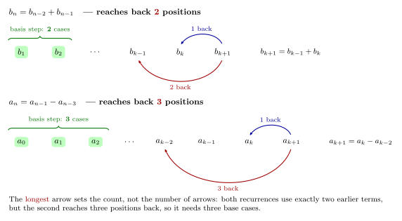
Figure 254: How many base cases a strong induction needs, on the two sequences worked below: b_n = b_{n-2} + b_{n-1} and a_n = a_{n-1} − a_{n-3}. Both use exactly two earlier terms, so counting terms gives the wrong answer; what settles it is the longest arrow. Reaching two positions back means the basis step must cover two cases; reaching three means three. The terms sit in a row, and each short curved arrow is labelled with what it does.
If the basis step establishes fewer cases than the inductive step consumes, the chain has a hole in it: the first few applications of the inductive step would reach for a case nobody ever proved.
Worked example — a two-term recurrence
Suppose \(b_1, b_2, b_3, \dots\) is defined by \(b_1 = 4\), \(b_2 = 12\), and \(b_n = b_{n-2} + b_{n-1}\) for each integer \(n \geq 3\). Prove that \(4 \mid b_n\) for each integer \(n \geq 1\).
Proof. Let \(P(n)\) be the predicate \(4 \mid b_n\).
Basis step. We know that \(b_1 = 4\) and \(b_2 = 12\). Since \(4 \mid 4\) and \(4 \mid 12\), \(P(1)\) is true and \(P(2)\) is true.
Inductive hypothesis. Suppose \(k \geq 2\) is an integer and that \(P(1), P(2), \dots, P(k)\) are true. Since \(P(k)\) is true, \(b_k = 4x\) for some \(x \in \mathbb{Z}\). Since \(P(k-1)\) is true, \(b_{k-1} = 4y\) for some \(y \in \mathbb{Z}\).
Inductive step. Consider \(n = k+1\):
\[b_{k+1} = b_{k-1} + b_k = 4y + 4x \qquad \text{(by the inductive hypothesis)}\] \[= 4(y+x)\]
Thus \(4 \mid b_{k+1}\), so \(P(k+1)\) is true.
Therefore, by PSMI, for each integer \(n \geq 1\), \(4 \mid b_n\). \(\square\)
Note where strong induction actually earns its keep: the step uses \(P(k)\) and \(P(k-1)\). Ordinary induction only hands you \(P(k)\), which is not enough to say anything about \(b_{k-1}\).
Worked example — every integer \(n > 1\) is a product of primes
Theorem. Every integer \(n > 1\) can be written as a product of primes.
Proof. Let \(P(n)\) be the predicate \(n\) can be written as a product of primes, for \(n \geq 2\).
Basis step. \(n = 2\) is prime and thus is a product of primes, so \(P(2)\) is true.
Inductive step. Suppose that for some integer \(k \geq 2\), every integer \(2, 3, \dots, k\) can be written as a product of primes — that is, \(P(2) \wedge P(3) \wedge \cdots \wedge P(k)\). We now need to prove that \(k+1\) is a product of primes. Since \(k + 1 > 1\), either \(k+1\) is prime or \(k+1\) is composite.
- Case 1: \(k+1\) is prime. Then \(k+1\) is a product of primes.
- Case 2: \(k+1\) is composite. Then \(k+1 = rs\) for some positive integers \(r \neq 1\) and \(s \neq 1\). This implies \(1 < r < k+1\) and \(1 < s < k+1\). So by the inductive hypothesis — specifically \(P(r)\) and \(P(s)\) — both \(r\) and \(s\) are products of primes. Let \(r = p_1p_2\dots p_a\) and \(s = q_1q_2\dots q_b\) where the \(p_i\) and \(q_j\) are primes; thus \(k+1 = rs = p_1p_2\dots p_a q_1q_2 \dots q_b\) is a product of primes.
In either case, \(k+1\) is a product of primes.
Therefore, by SMI, every integer \(n > 1\) can be written as a product of primes. \(\square\)
Why strong induction and not ordinary induction? Because \(r\) and \(s\) can be any integers from 2 to \(k\) — the factorisation gives no control over which — so the proof needs the inductive hypothesis available at all of those values, not just at \(k\).
The well-ordering principle for the integers
Let \(S\) be a non-empty set of integers, each of which is greater than some fixed integer. Then \(S\) has a least element.
Four pieces of terminology, all load-bearing:
- non-empty — the empty set has no least element, trivially.
- of integers — not of rationals or reals. This clause is not decoration: the positive rationals are non-empty and bounded below by 0, and still have no least element, because between any candidate and 0 there is always another one (halve it). See 2026-08-27-strong-induction-and-well-ordering.
- greater than some fixed integer — \(S\) must be bounded below. Without this the principle fails: \(\mathbb{Z}^-\) is a non-empty set of integers with no least element.
- a least element — an element of \(S\) that is \(\leq\) every element of \(S\). It lives inside the set, not outside it.
Example — integers congruent to \(1 \bmod 4\)
True or false? The set of all integers congruent to \(1 \bmod 4\) has a least element.
False. The set is \(\{\dots, -7, -3, 1, 5, 9, \dots\}\).
Suppose this set did have a least element, call it \(x\). Then, since \(x \equiv 1 \pmod 4\), we have \(x - 4 \equiv 1 \pmod 4\), so \(x-4\) is also in the set. But \(x - 4\) is smaller than \(x\) — a contradiction. \(\square\)
The set is non-empty, but it fails the “bounded below” condition, so the well-ordering principle simply does not apply to it.
MI, SMI and the WOP are equivalent
Anything provable by one is provable by the other two. Two of the translations:
SMI \(\to\) MI: reword the statement. A strong-induction proof of \(P(n)\) becomes an ordinary-induction proof of the accumulated predicate
\[Q(n) \;\equiv\; P(0) \wedge P(1) \wedge \cdots \wedge P(n)\]
Assuming \(Q(k)\) in ordinary induction gives you exactly what assuming \(P(0), \dots, P(k)\) gave you in strong induction. (Epp, Q27 p. 279.)
MI \(\to\) WOP: argue by contradiction. Suppose the set of integers \(\geq a\) for which \(P(n)\) is false is non-empty. It is bounded below by \(a\), so by the WOP it has a least element; derive a contradiction from that least element. (Epp, Q31 p. 279.)
The same theorem, three ways
Suppose \(a_0, a_1, a_2, \dots\) is defined by \(a_0 = 6\), \(a_1 = 9\), \(a_2 = 12\) and \(a_n = a_{n-1} - a_{n-3}\) for each integer \(n \geq 3\). Prove that for all integers \(n \geq 0\), \(3 \mid a_n\).
By SMI.
Let \(P(n)\) be the predicate \(3 \mid a_n\).
Basis step. \(a_0 = 6\), \(a_1 = 9\) and \(a_2 = 12\). Since \(3 \mid 6\), \(3 \mid 9\) and \(3 \mid 12\), \(P(0)\), \(P(1)\) and \(P(2)\) are true.
Inductive hypothesis. Suppose \(k \geq 2\) is an integer and that \(P(0), P(1), \dots, P(k)\) are true. Since \(P(k-2)\) is true, \(a_{k-2} = 3y\) for some \(y \in \mathbb{Z}\); since \(P(k)\) is true, \(a_k = 3x\) for some \(x \in \mathbb{Z}\).
Inductive step. Consider \(n = k+1\): \(a_{k+1} = a_k - a_{k-2} = 3x - 3y = 3(x-y)\). Thus \(3 \mid a_{k+1}\), so \(P(k+1)\) is true.
Therefore, by PSMI, for each integer \(n \geq 0\), \(3 \mid a_n\). \(\square\)
By MI, on the reworded predicate.
Let \(Q(n)\) be the predicate \(3 \mid a_j\) for all integers \(j\) where \(0 \leq j \leq n\) — that is, \(Q(n) \equiv P(0) \wedge P(1) \wedge \cdots \wedge P(n)\).
Basis step. Consider \(n = 2\). Since \(3 \mid a_0\), \(3 \mid a_1\) and \(3 \mid a_2\), \(Q(2)\) is true.
Inductive hypothesis. Suppose \(k \geq 2\) is an integer and that \(Q(k)\) is true. Since \(Q(k)\) is true and \(k \geq 2\), \(a_k = 3x\) and \(a_{k-2} = 3y\) for some \(x, y \in \mathbb{Z}\).
Inductive step. Consider \(n = k+1\): \(a_{k+1} = a_k - a_{k-2} = 3x - 3y = 3(x-y)\). Thus \(3 \mid a_{k+1}\). Since \(Q(k)\) already gives \(3 \mid a_i\) for every \(0 \leq i \leq k\), adding \(3 \mid a_{k+1}\) gives \(Q(k+1)\).
(That last step is the point of rewording the predicate: \(Q(k+1)\) is a conjunction over all indices up to \(k+1\), so it needs \(Q(k)\) and the new case — \(3 \mid a_{k+1}\) alone would not establish it.)
Therefore, by PMI, for each integer \(n \geq 0\), \(3 \mid a_n\). \(\square\)
The two proofs have the same algebraic core: the line \(a_{k+1} = a_k - a_{k-2} = 3x - 3y = 3(x-y)\) is identical in each. All the reworded predicate does is let a single assumption, \(Q(k)\), carry the several earlier facts the algebra needs.
Two details of the MI proof are easy to get wrong:
- The basis is \(n = 2\), not \(n = 0\). \(Q(2)\) already asserts \(3 \mid a_0\), \(3 \mid a_1\) and \(3 \mid a_2\), so verifying \(Q(2)\) discharges all three of the SMI proof’s base cases in one statement. Three base cases have not disappeared; they have been packed into one predicate.
- The step concludes \(Q(k+1)\), not \(P(k+1)\). An ordinary induction on \(Q\) has to deliver \(Q(k+1)\), and \(3 \mid a_{k+1}\) on its own does not — it needs \(Q(k)\) alongside it.
The conjunction in \(Q\) starts at \(P(0)\), not \(P(1)\). The predicate is \(3 \mid a_j\) for all integers \(j\) where \(0 \leq j \leq n\), so \(Q(2) \equiv P(0) \wedge P(1) \wedge P(2)\) — which is also what the basis step checks.
By the WOP, by contradiction.
Suppose the statement is false, so there exists an integer \(n \geq 0\) such that 3 does not divide \(a_n\). Let
\[A = \{\, n \in \mathbb{Z}^{\geq 0} \;:\; 3 \nmid a_n \,\}\]
By the WOP and our assumption, \(A\) has a least element — the smallest \(n\) for which \(3 \nmid a_n\). Call it \(k\). Thus \(3 \nmid a_k\), but \(3 \mid a_i\) for all \(0 \leq i \leq k-1\).
Note that \(k \geq 3\), since \(a_0\), \(a_1\) and \(a_2\) are all divisible by 3.
Thus \(a_{k-1} = 3x\) and \(a_{k-3} = 3y\) for some \(x, y \in \mathbb{Z}\), so
\[a_k = a_{k-1} - a_{k-3} = 3x - 3y = 3(x-y)\]
Thus \(3 \mid a_k\), which is a contradiction.
Therefore, for each integer \(n \geq 0\), \(3 \mid a_n\). \(\square\)
Reading the WOP proof next to the SMI one: “let \(k\) be the least counterexample” plays the role of the inductive hypothesis (everything below \(k\) works), and “\(3 \mid a_k\), contradiction” plays the role of the inductive step. Drawn on the index line, the whole proof is one picture:
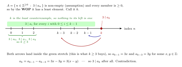
Figure 255: The well-ordering proof of 3 | a_n as a picture of its own least counterexample. Everything to the left of k is green not because it was proved, but because k was chosen least — that single step is the only place the WOP is used, and it is exactly what the strong inductive hypothesis supplies in the SMI proof. The least element here is the smallest number that gives a contradiction. k ≥ 3 is what guarantees both arrows land inside the green stretch, since a_{k-3} has to be a term of the sequence at all.
Note which term the WOP proof reaches for. The SMI proof used \(a_k\) and \(a_{k-2}\) to build \(a_{k+1}\); the WOP proof is standing at \(k\) rather than at \(k+1\), so the same recurrence reads \(a_k = a_{k-1} - a_{k-3}\) and it reaches for \(a_{k-1}\) and \(a_{k-3}\). Same recurrence, index shifted by one — and that shift is why the “\(k \geq 3\)” line has to be there.
Spotting a WOP proof
A proof is using the well-ordering principle whenever it says “choose the smallest such \(n\)” about a set it has just argued is non-empty. That phrase is not free — it is the WOP being invoked, and it needs the set to be non-empty and bounded below.
For instance, the primes theorem above can be rewritten as a contradiction proof: suppose some integer \(n > 1\) is not a product of primes; by the WOP, choose the smallest such \(n\); then \(n\) is prime (done) or \(n = rs\) with \(1 < r, s < n\), and both \(r\) and \(s\) are products of primes precisely because \(n\) was chosen smallest — contradicting the choice of \(n\). Structurally it is the SMI proof with the induction turned inside out.
See also
- mathematical-induction · proof-techniques · sequences-and-summations
- recursive-definitions · solving-recurrence-relations — where a two-term recurrence forces the strong hypothesis
- trees — strong induction on the number of vertices: a tree with \(n\) vertices has \(n - 1\) edges
- 2026-08-27-strong-induction-and-well-ordering — Lecture 14
- practice-problems — §18, with full worked solutions
Subgroups and Cyclic Groups
A subgroup is a group sitting inside another group under the same operation. The quickest way to build one is to take a single element and all of its powers, positive, zero and negative: that set is the cyclic subgroup the element generates. A group that is the cyclic subgroup of one of its own elements is a cyclic group. The definition of a group is in [groups], and most of the examples live in integers-modulo-n. First met in 2026-10-06-elementary-properties-of-groups, and cyclic groups are also worked in 2026-10-08-definitions-and-examples-of-fields.
Subgroups
Definition. If \((G, *)\) is a group and \(H \subseteq G\), then \(H\) is a subgroup of \(G\) if \((H, *)\) is itself a group.
To check that \((H, *)\) is a subgroup of \((G, *)\), check three of the four group properties:
| Property | To show it holds | To show it fails |
|---|---|---|
| closure | Take arbitrary \(g, h \in H\) and show \(g * h \in H\). | Two elements of \(H\) whose result is outside \(H\). |
| identity | Show that the identity \(e\) of \(G\) is in \(H\). | Show \(e \notin H\). |
| inverses | Take arbitrary \(h \in H\) and show its inverse in \(G\) is in \(H\). | One element of \(H\) whose inverse is outside \(H\). |
Associativity is inherited. \((g * h) * k = g * (h * k)\) holds for all \(g, h, k \in G\), and elements of \(H\) are elements of \(G\), so it holds for all \(g, h, k \in H\). Nothing new has to be checked. The other three properties are different: each one says some element must be in the set, and a smaller set can leave it out.
Points to watch:
- The same operation. \(\mathbb{R} - \{0\}\) is a group under multiplication, but it is not a subgroup of \((\mathbb{R}, +)\): under \(+\) it is not closed, since \(1 + (-1) = 0\), and it has no identity (2026-10-06-elementary-properties-of-groups).
- The identity of \(H\) is the identity of \(G\). If some \(f \in H\) worked as an identity for \(H\), then \(f * f = f = f * e\) in \(G\), and cancelling \(f\) on the left (groups) gives \(f = e\). So the identity check is simply: is \(e \in H\)? It also makes sure \(H\) is not empty.
- The inverse of \(h\) in \(H\) is its inverse in \(G\), for the same reason: inverses in a group are unique (groups). So the inverses check is: for each \(h \in H\), is \(h^{-1} \in H\)?
Every group has two subgroups for free: \(\{e\}\), and \(G\) itself.
| \(H\) | \(G\) | Subgroup? | Why |
|---|---|---|---|
| \(\mathbb{Z}\) | \((\mathbb{R}, +)\) | yes | \(a + b \in \mathbb{Z}\), \(\ 0 \in \mathbb{Z}\), \(\ -a \in \mathbb{Z}\) (2026-10-06-elementary-properties-of-groups) |
| \(\mathbb{R} - \{0\}\) | \((\mathbb{R}, +)\) | no | \(1 + (-1) = 0 \notin H\), and \(0\), the identity, is missing |
| \(\{3n : n \in \mathbb{Z}\}\) | \((\mathbb{Z}, +)\) | yes | \(3a + 3b = 3(a + b)\), \(\ 0 = 3 \cdot 0\), \(\ -3a = 3(-a)\) |
| \(\{[0], [2], [4]\}\) | \((\mathbb{Z}_6, +)\) | yes | its block of the table uses only its own elements (cayley-tables) |
| \(\{[0], [1]\}\) | \((\mathbb{Z}_6, +)\) | no | \([1] + [1] = [2] \notin H\) |
The multiples of 3 are Q1 of practice-problems, worked there in full.
Powers of an element
If \((G, *)\) is a group and \(a \in G\), then \(a^i\) is defined for each \(i \in \mathbb{Z}\) as follows:
\(a^0 = e\), where \(e\) is the identity of \(G\);
\(a^i = \underbrace{a * a * \cdots * a}_{i \text{ times}}\) for each \(i \in \mathbb{Z}^{+}\);
\(a^{-i} = \underbrace{a^{-1} * a^{-1} * \cdots * a^{-1}}_{i \text{ times}}\) for each \(i \in \mathbb{Z}^{+}\).
A positive power combines \(a\) with itself; a negative power does the same with the inverse \(a^{-1}\); and the zero power is the identity, the result of combining nothing. The definition agrees with itself at \(i = 1\): \(a^1 = a\), and \(a^{-1}\) is one copy of the inverse of \(a\), which is what \(a^{-1}\) already meant.
The notation does not change with the operation, and in an additive group that takes care:
| Group | \(a^2\) | \(a^3\) | \(a^0\) | \(a^{-1}\) |
|---|---|---|---|---|
| \((\mathbb{R} - \{0\}, \cdot)\) | \(a \cdot a\) | \(a \cdot a \cdot a\) | \(1\) | \(\frac1a\) |
| \((\mathbb{Z}, +)\) | \(a + a = 2a\) | \(3a\) | \(0\) | \(-a\) |
| \((\mathbb{Z}_{12}, +)\), \(a = 3\) | \(3 + 3 = 6\) | \(9\) | \(0\) | \(-3 = 9\) |
| \((S_3, \circ)\), \(a = f_5\) | \(f_5 \circ f_5 = f_6\) | \(f_1\) | \(f_1\) | \(f_6\) |
In an additive group the powers of \(a\) are its multiples, \(a^n = na\), and \(a^{-1} = -a\). “\(3^2\)” in \((\mathbb{Z}_{12}, +)\) is \(6\), not \(9\).
The power laws
For all \(g \in G\) and all \(i, j \in \mathbb{Z}\):
\[g^i * g^j = g^{i + j} \qquad\qquad (g^i)^{-1} = g^{-i} = (g^{-1})^i.\]
Why the first law holds. When \(i\) and \(j\) are both positive it is counting: \(i\) copies of \(g\) followed by \(j\) copies make \(i + j\) copies. When the signs differ, the \(g\)s and \(g^{-1}\)s meet in the middle and cancel in pairs, \(g * g^{-1} = e\), and what is left is the surplus. For example
\[g^3 * g^{-2} = g * g * \underbrace{g * g^{-1}}_{e} * g^{-1} = g * \underbrace{g * g^{-1}}_{e} = g = g^{3 + (-2)}.\]
A zero power is \(e\) and changes nothing, matching \(i + 0 = i\).
Why the second. \(i\) copies of \(g\) followed by \(i\) copies of \(g^{-1}\) cancel completely, so \(g^i * g^{-i} = g^0 = e\), and in the other order \(g^{-i} * g^i = g^0 = e\). That makes \(g^{-i}\) the inverse of \(g^i\). And \((g^{-1})^i\) is \(i\) copies of \(g^{-1}\), which is \(g^{-i}\) by definition.
The laws say powers in a group behave like powers of a number. They are what the cyclic subgroup needs.
Worked: one negative power, three ways
\([3]^{-4}\) in \((\mathbb{Z}_7 - \{[0]\}, \cdot)\), where \([3]^4 = [81] = [4]\) (2026-10-06-elementary-properties-of-groups):
- Invert, then power. \([3]^{-1} = [5]\), because \([3] \cdot [5] = [15] = [1]\). So \([3]^{-4} = [5]^4 = [25] \cdot [25] = [4] \cdot [4] = [2]\).
- Power, then invert. \([3]^{-4} = ([3]^4)^{-1} = [4]^{-1} = [2]\), because \([4] \cdot [2] = [8] = [1]\).
- Go round the loop. The powers of \([3]\) are \([3], [2], [6], [4], [5], [1]\), so \([3]^6 = [1]\). Then \([3]^{-4} = [3]^{-4} \cdot [3]^6 = [3]^2 = [9] = [2]\).
All three give \([2]\). The third uses the fact that the powers in a finite group come round in a loop, which is the next section.
When the powers repeat
In a finite group, some positive power of \(a\) is \(e\). The powers \(a, a^2, a^3, \ldots\) cannot all be different, so \(a^i = a^j\) for some \(0 < i < j\). Combine both sides with \(a^{-i}\): \(e = a^{j - i}\), a positive power.
Let \(n\) be the smallest positive integer with \(a^n = e\). Then:
- \(a, a^2, \ldots, a^n\) are all different. If \(a^i = a^j\) with \(1 \le i < j \le n\), the same step gives \(a^{j-i} = e\) with \(0 < j - i < n\), smaller than \(n\).
- After \(a^n\) the list repeats. \(a^{n+1} = a^n * a = e * a = a\), then \(a^{n+2} = a^2\), and so on.
- The negative powers are already in the list. \(a^{n-1} * a = a^n = e\), so \(a^{-1} = a^{n-1}\), and in general \(a^{-i} = a^{n-i}\). Going backwards round the loop meets the same elements.
So in a finite group
\[\langle a \rangle = \{a, a^2, a^3, \ldots, a^n = e\},\]
with exactly \(n\) elements: list the positive powers until \(e\) appears, and stop. (\(n\) is often called the order of \(a\).) In an infinite group the powers need not repeat, and then the negative powers really are new.
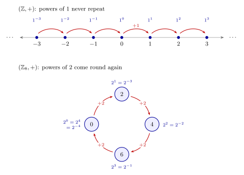
Figure 256: Powers of an element as steps, each step combining with the element once more; going left or backwards combines with its inverse. Top: in \((\mathbb{Z}, +)\) the powers of \(1\) run off in both directions and never repeat, so \(\langle 1 \rangle\) needs the negative powers to reach \(-1, -2, \ldots\). Bottom: in \((\mathbb{Z}_8, +)\) the powers of \(2\) come back to the identity at \(2^4 = 0\), so the line closes into a loop of four. Every negative power lands on a positive one, such as \(2^{-1} = 6 = 2^3\), and \(\langle 2 \rangle = {2, 4, 6, 0}\) is just the positive powers up to the identity.
The cyclic subgroup generated by \(a\)
If \((G, *)\) is a group and \(a \in G\), then \[\langle a \rangle = \{a^i : i \in \mathbb{Z}\}\] is a subgroup of \(G\), and is called the cyclic subgroup of \(G\) generated by \(a\).
Why it is a subgroup. The power laws are exactly the three checks.
- Closure. \(a^i * a^j = a^{i + j}\), and \(i + j \in \mathbb{Z}\), so it is in \(\langle a \rangle\).
- Identity. \(e = a^0 \in \langle a \rangle\).
- Inverses. \((a^i)^{-1} = a^{-i} \in \langle a \rangle\).
It is the smallest subgroup containing \(a\). Suppose \(S\) is any subgroup with \(a \in S\). Closure puts \(a^2, a^3, a^4, \ldots\) in \(S\). The identity puts \(a^0 = e\) in \(S\). Inverses put \(a^{-1}\) in \(S\), and then closure puts \(a^{-2}, a^{-3}, \ldots\) in \(S\). So \(\langle a \rangle \subseteq S\). A subgroup cannot contain \(a\) without containing all of its powers.
Two rules that save work:
- \(\langle e \rangle = \{e\}\). Every power of the identity is the identity.
- \(\langle a \rangle = \langle a^{-1} \rangle\). The powers of \(a^{-1}\) are \((a^{-1})^i = a^{-i}\), and as \(i\) runs through all of \(\mathbb{Z}\) so does \(-i\). The same set, listed in the opposite order. In \((\mathbb{Z}_n, +)\) the inverse of \(a\) is \(n - a\), so \(\langle a \rangle = \langle n - a \rangle\).
To find \(\langle a \rangle\) in a finite group, list \(a, a^2, a^3, \ldots\), each one the previous one combined with \(a\), until the identity appears (above).
Worked examples
\(\langle 3 \rangle\) in \((\mathbb{Z}_{11} - \{[0]\}, \cdot)\). The powers are \(3, 9, 27 = 5, 15 = 4, 12 = 1\), so \(\langle 3 \rangle = \{1, 3, 4, 5, 9\}\), five of the ten elements. Worked and drawn in 2026-10-06-elementary-properties-of-groups.
All the cyclic subgroups of \((\mathbb{Z}_8, +)\) (2026-10-06-elementary-properties-of-groups):
| \(a\) | Powers of \(a\) until \(0\) | \(\langle a \rangle\) | Size |
|---|---|---|---|
| \(0\) | \(0\) | \(\{0\}\) | 1 |
| \(1\), \(7\) | \(1, 2, 3, 4, 5, 6, 7, 0\) | \(\mathbb{Z}_8\) | 8 |
| \(3\), \(5\) | \(3, 6, 1, 4, 7, 2, 5, 0\) | \(\mathbb{Z}_8\) | 8 |
| \(2\), \(6\) | \(2, 4, 6, 0\) | \(\{0, 2, 4, 6\}\) | 4 |
| \(4\) | \(4, 0\) | \(\{0, 4\}\) | 2 |
The rows pair each element with its inverse (\(7 = -1\), \(5 = -3\), \(6 = -2\)), which generates the same subgroup. Eight elements, four different cyclic subgroups, nested one inside the next: \(\{0\} \subset \{0, 4\} \subset \{0, 2, 4, 6\} \subset \mathbb{Z}_8\).
All the cyclic subgroups of \((\mathbb{Z}_6, +)\). By the same method, \(\langle 0 \rangle = \{0\}\), \(\ \langle 1 \rangle = \langle 5 \rangle = \mathbb{Z}_6\), \(\ \langle 2 \rangle = \langle 4 \rangle = \{0, 2, 4\}\) and \(\langle 3 \rangle = \{3, 0\}\). The subgroup \(\langle 2 \rangle = \{0, 2, 4\}\) is the block in the table at 2026-10-06-elementary-properties-of-groups.
Cyclic groups
The group \((G, *)\) is cyclic if there exists an \(a \in G\) such that \(\langle a \rangle = G\).
Such an \(a\) is a generator of \(G\). A cyclic group is one in which every element is a power of one element.
- To prove \(G\) is cyclic, name a generator \(a\) and show every element of \(G\) is a power of it. In a finite group, list the powers of \(a\) until the identity appears and count: if there are \(|G|\) different ones, \(\langle a \rangle = G\).
- To prove \(G\) is not cyclic, show that \(\langle a \rangle \neq G\) for every \(a \in G\). One element that fails to generate proves nothing.
| Group | Cyclic? | Generators found | Where |
|---|---|---|---|
| \((\mathbb{Z}_{10}, +)\) | yes | \(1\) | 2026-10-06-elementary-properties-of-groups |
| \((\mathbb{Z}_8, +)\) | yes | \(1, 3, 5, 7\) | 2026-10-06-elementary-properties-of-groups |
| \((\mathbb{Z}_6, +)\) | yes | \(1, 5\) | above |
| \((\mathbb{Z}_5 - \{[0]\}, \cdot)\) | yes | \(2, 3\) | 2026-10-06-elementary-properties-of-groups |
| \((\mathbb{Z}_{11} - \{[0]\}, \cdot)\) | yes | \(2\), but not \(3\) | practice-problems, Q4 |
| \((\mathbb{Z}, +)\) | yes | \(1, -1\) | 2026-10-06-elementary-properties-of-groups |
| \((\mathbb{Z}_2 \times \mathbb{Z}_3, +)\) | yes | \((1, 1)\), \((1, 2)\) | below |
| \((\mathbb{Q}, +)\) | no | none | below |
| \((S_3, \circ)\) | no | none | symmetric-group |
\((\mathbb{Z}_n, +)\) is always cyclic, generated by \(1\): the powers of \(1\) are \(1, 2, \ldots, n - 1, n = 0\).
\((\mathbb{Z}, +)\) needs the negative powers. \(\langle 1 \rangle = \{\ldots, 1^{-2}, 1^{-1}, 1^0, 1^1, 1^2, \ldots\} = \{\ldots, -2, -1, 0, 1, 2, \ldots\} = \mathbb{Z}\). The positive powers alone give only \(\mathbb{Z}^{+}\).
A cyclic group is abelian. Any two elements are powers \(a^i\) and \(a^j\) of the generator, and \(a^i * a^j = a^{i + j} = a^{j + i} = a^j * a^i\). So a non-abelian group, such as \(S_3\), cannot be cyclic.
Worked: \((\mathbb{Q}, +)\) is not cyclic
In \((\mathbb{Q}, +)\) the powers of \(a\) are its integer multiples, \(\langle a \rangle = \{na : n \in \mathbb{Z}\}\). Take any \(a \in \mathbb{Q}\).
- If \(a = 0\), then \(\langle a \rangle = \{0\} \neq \mathbb{Q}\).
- If \(a = \frac{p}{q} \neq 0\), with \(p, q \in \mathbb{Z}\) and \(q \neq 0\), then \(\frac{p}{2q} \in \mathbb{Q}\). If it were in \(\langle a \rangle\), then \(\frac{p}{2q} = n \cdot \frac{p}{q}\) for some \(n \in \mathbb{Z}\), and dividing by \(\frac{p}{q} \neq 0\) gives \(n = \frac12\), which is not an integer. So \(\frac{p}{2q} \notin \left\langle \frac{p}{q} \right\rangle\).
No \(a\) generates \(\mathbb{Q}\), so \((\mathbb{Q}, +)\) is not cyclic. The same argument works for \((\mathbb{R}, +)\).
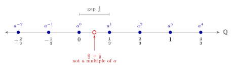
Figure 257: Why no rational number generates \((\mathbb{Q}, +)\), drawn for \(a = \tfrac13\). The powers of \(a\) under addition are its integer multiples, evenly spaced points a distance \(\tfrac13\) apart running off in both directions. Half of \(a\), here \(\tfrac16\), is a rational number that falls in the gap between \(a^0 = 0\) and \(a^1 = \tfrac13\), so it is not a power of \(a\). Any other non-zero \(a\) has gaps of the same kind, and \(a = 0\) generates only \({0}\).
Worked: \(\mathbb{Z}_2 \times \mathbb{Z}_3\) is cyclic
In \((\mathbb{Z}_2 \times \mathbb{Z}_3, +)\), with \((a, b) + (c, d) = \big((a + c) \bmod 2,\ (b + d) \bmod 3\big)\), the powers of \((1, 1)\) are
\[(1,1),\ (0,2),\ (1,0),\ (0,1),\ (1,2),\ (0,0),\]
six different elements, so \(\langle (1, 1) \rangle\) is the whole group and it is cyclic (2026-10-06-elementary-properties-of-groups). Each step adds 1 to both coordinates. The first coordinate is back at \(0\) after every 2 steps, the second after every 3, and both are back together for the first time after 6, so the powers visit all six pairs before returning to \((0, 0)\). Elements that move only one coordinate generate smaller subgroups:
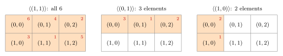
Figure 258: Three cyclic subgroups of \(\mathbb{Z}_2 \times \mathbb{Z}_3\), each shaded inside the six-element group. A shaded cell is a power of the generator, and the small number in its corner is the \(k\) at which the generator’s \(k\)th power first lands there. Left: \((1,1)\) changes both coordinates at every step and reaches all six pairs before \((1,1)^6 = (0,0)\), so it generates the whole group and the group is cyclic. Middle: \((0,1)\) never changes the first coordinate, so its powers stay in the top row and \(\langle (0,1) \rangle\) has three elements. Right: \((1,0)\) never changes the second coordinate, so \(\langle (1,0) \rangle = {(0,0), (1,0)}\).
\((1, 2)\) is a second generator, since it is the inverse of \((1, 1)\): \((1,1) + (1,2) = (2 \bmod 2,\ 3 \bmod 3) = (0, 0)\). Of the other non-identity elements, \((0, 1)\) and its inverse \((0, 2)\) both generate \(\langle (0, 1) \rangle\), and \((1, 0)\), which is its own inverse, generates \(\langle (1, 0) \rangle\).
Common mistakes
- Checking associativity for a subgroup. It is inherited from \(G\) and never fails. The three that need checking are closure, identity and inverses.
- Forgetting that \(e\) must be in \(H\). \(\mathbb{R} - \{0\}\) fails as a subgroup of \((\mathbb{R}, +)\) because the identity was removed.
- Changing the operation. A subgroup of \((G, *)\) uses \(*\). \((\mathbb{R} - \{0\}, \cdot)\) is a group, but not a subgroup of \((\mathbb{R}, +)\).
- Reading \(a^2\) as \(a \cdot a\) in an additive group. In \((\mathbb{Z}_{12}, +)\), \(3^2 = 3 + 3 = 6\).
- Reading \(a^{-1}\) as \(\frac1a\). It is the inverse under the group’s operation: \(-a\) in an additive group.
- Leaving out the negative powers in an infinite group. The positive powers of \(1\) in \((\mathbb{Z}, +)\) are only \(1, 2, 3, \ldots\).
- Confusing \(\langle a \rangle\) with \(\{a\}\). \(\langle a \rangle\) contains every power of \(a\), including \(e\).
- “\(3\) does not generate it, so it is not cyclic.” One generator is enough to be cyclic. \(\mathbb{Z}_{11} - \{[0]\}\) is \(\langle 2 \rangle\) though not \(\langle 3 \rangle\). To show a group is not cyclic, every element must fail.
- Expecting the identity to generate. \(\langle e \rangle = \{e\}\), in every group.
See also
- [groups] — the four properties, and the elementary properties such as the unique identity and \((g * h)^{-1} = h^{-1} * g^{-1}\)
- cayley-tables — a subgroup as a block of the table, when its elements are listed first
- integers-modulo-n — \(\mathbb{Z}_n\) and \(\mathbb{Z}_n - \{[0]\}\), where most of the cyclic examples live
- symmetric-group — the cyclic subgroups of \(S_3\), a group that is not cyclic
- 2026-10-06-elementary-properties-of-groups — Lecture 27 · 2026-10-08-definitions-and-examples-of-fields — Lecture 28
- practice-problems — §34, with full worked solutions
The Symmetric Group
\(S_n\) is the group whose elements are the bijections from \(\{1, 2, \dots, n\}\) to itself, and whose operation is composition. Its elements are functions, not numbers, and it is the course’s first group in which the order of a product matters. The definition of a group is in [groups], and the two ingredients are one-to-one-and-onto-functions and composition-of-functions. First met in 2026-09-24-definitions-and-examples-of-groups.
The definition
\(S_n\) is the group consisting of the set of all bijections from \(\{1, 2, \cdots, n\}\) to \(\{1, 2, \cdots, n\}\) together with the binary operation \(\circ\) denoting composition of functions.
An element of \(S_n\) is a way of sending each of \(1, \dots, n\) to one of \(1, \dots, n\), so that no two go to the same place and every place is used. To combine two elements, do one and then the other.
How many elements. A bijection in \(S_3\) can send 1 to any of three places. That leaves two places for 2, and then one for 3, so \(S_3\) has \(3 \cdot 2 \cdot 1 = 6\) elements. In general \(S_n\) has \(n!\) elements, one for each arrangement of \(1, \dots, n\) (counting-principles).
The six elements of \(S_3\)
They are named \(f_1\) to \(f_6\) here, and each can be drawn as an arrow diagram (2026-09-24-definitions-and-examples-of-groups). Each can also be written as a set of pairs or as a list of values.
| As a set of pairs | \(1 \mapsto\) | \(2 \mapsto\) | \(3 \mapsto\) | What it does | |
|---|---|---|---|---|---|
| \(f_1\) | \(\{(1,1),(2,2),(3,3)\}\) | 1 | 2 | 3 | nothing |
| \(f_2\) | \(\{(1,2),(2,1),(3,3)\}\) | 2 | 1 | 3 | swaps 1 and 2 |
| \(f_3\) | \(\{(1,3),(2,2),(3,1)\}\) | 3 | 2 | 1 | swaps 1 and 3 |
| \(f_4\) | \(\{(1,1),(2,3),(3,2)\}\) | 1 | 3 | 2 | swaps 2 and 3 |
| \(f_5\) | \(\{(1,2),(2,3),(3,1)\}\) | 2 | 3 | 1 | moves all three |
| \(f_6\) | \(\{(1,3),(2,1),(3,2)\}\) | 3 | 1 | 2 | moves all three, the other way |
The pair form is the definition of a function as a set of pairs (functions-on-general-sets). The names \(f_1, \dots, f_6\) are just labels, and other sources number the six differently.
Composing
\[(f \circ g)(x) = f(g(x))\]
The function on the right acts first. To work out \(f \circ g\), take each of 1, 2, 3 in turn, apply \(g\), then apply \(f\) to the result.
\(f_2 \circ f_3\): \(f_3\) first, then \(f_2\).
| \(x\) | \(f_3(x)\) | \(f_2(f_3(x))\) |
|---|---|---|
| 1 | 3 | 3 |
| 2 | 2 | 1 |
| 3 | 1 | 2 |
So \(f_2 \circ f_3\) sends \(1 \mapsto 3\), \(2 \mapsto 1\), \(3 \mapsto 2\), which is \(f_6\).
\(f_3 \circ f_2\): \(f_2\) first, then \(f_3\).
| \(x\) | \(f_2(x)\) | \(f_3(f_2(x))\) |
|---|---|---|
| 1 | 2 | 2 |
| 2 | 1 | 3 |
| 3 | 3 | 1 |
So \(f_3 \circ f_2\) sends \(1 \mapsto 2\), \(2 \mapsto 3\), \(3 \mapsto 1\), which is \(f_5\).
The same two functions in the two orders give different answers. \(f_2 \circ f_3 = f_6\) but \(f_3 \circ f_2 = f_5\).
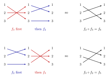
Figure 259: The same two elements of \(S_3\) composed in both orders. Top: \(f_3\) first and then \(f_2\), which is \(f_2 \circ f_3\). Following each number through both steps gives \(1 \to 3\), \(2 \to 1\), \(3 \to 2\), the element \(f_6\). Bottom: \(f_2\) first and then \(f_3\), which is \(f_3 \circ f_2\). Now the result is \(1 \to 2\), \(2 \to 3\), \(3 \to 1\), the element \(f_5\). In each row the picture runs left to right in the order things happen, and the formula names the functions right to left.
Why it is a group
For \(S_3\) the properties can be checked from its table, with associativity by a general argument (2026-09-24-definitions-and-examples-of-groups). Each one also follows, for every \(n\), from facts about functions:
- Closure. The composition of two bijections is a bijection (composition-of-functions).
- Associativity. For any three functions, \(f \circ (g \circ h)\) and \((f \circ g) \circ h\) both send \(x\) to \(f(g(h(x)))\).
- Identity. The function that sends every number to itself, \(f_1\) in \(S_3\). Composing with it on either side changes nothing.
- Inverses. A bijection has an inverse function (inverse-functions), which is again a bijection, and composing the two in either order gives the identity (composition-of-functions).
So the inverse of \(f\) in the group \(S_n\) is the inverse function \(f^{-1}\), and the two uses of the notation agree. In an arrow diagram the inverse is found by reversing every arrow.
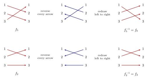
Figure 260: Inverses in \(S_3\) by reversing arrows. Top: \(f_5\) sends \(1 \to 2\), \(2 \to 3\), \(3 \to 1\). Turning each arrow round gives \(2 \to 1\), \(3 \to 2\), \(1 \to 3\), and reading that as a function of 1, 2, 3 gives \(1 \to 3\), \(2 \to 1\), \(3 \to 2\), which is \(f_6\). So \(f_5^{-1} = f_6\). Bottom: \(f_2\) swaps 1 and 2. Turning its arrows round gives the same diagram, so \(f_2\) is its own inverse. The same holds for \(f_3\) and \(f_4\), the other two swaps.
The Cayley table of \(S_3\)
The entry in the row of \(f\) and the column of \(g\) is \(f \circ g\) (cayley-tables).
| \(\circ\) | \(f_1\) | \(f_2\) | \(f_3\) | \(f_4\) | \(f_5\) | \(f_6\) |
|---|---|---|---|---|---|---|
| \(\mathbf{f}_1\) | \(f_1\) | \(f_2\) | \(f_3\) | \(f_4\) | \(f_5\) | \(f_6\) |
| \(\mathbf{f}_2\) | \(f_2\) | \(f_1\) | \(f_6\) | \(f_5\) | \(f_4\) | \(f_3\) |
| \(\mathbf{f}_3\) | \(f_3\) | \(f_5\) | \(f_1\) | \(f_6\) | \(f_2\) | \(f_4\) |
| \(\mathbf{f}_4\) | \(f_4\) | \(f_6\) | \(f_5\) | \(f_1\) | \(f_3\) | \(f_2\) |
| \(\mathbf{f}_5\) | \(f_5\) | \(f_3\) | \(f_4\) | \(f_2\) | \(f_6\) | \(f_1\) |
| \(\mathbf{f}_6\) | \(f_6\) | \(f_4\) | \(f_2\) | \(f_3\) | \(f_1\) | \(f_5\) |
Read off it:
- Identity: \(f_1\).
- Inverses: \(f_1^{-1} = f_1\), \(f_2^{-1} = f_2\), \(f_3^{-1} = f_3\), \(f_4^{-1} = f_4\), \(f_5^{-1} = f_6\), \(f_6^{-1} = f_5\).
- Not abelian: \(f_2 \circ f_3 = f_6\) but \(f_3 \circ f_2 = f_5\).
The three swaps are their own inverses: doing a swap twice puts everything back. \(f_5\) and \(f_6\) undo each other. The table also shows \(f_5 \circ f_5 = f_6\) and \(f_6 \circ f_5 = f_1\), so doing \(f_5\) three times returns everything to where it started.
Non-abelian does not mean nothing commutes. \(f_5 \circ f_6 = f_6 \circ f_5 = f_1\), and \(f_1\) commutes with everything. A group is non-abelian as soon as one pair fails to commute.
Powers and cyclic subgroups of \(S_3\)
Powers are defined in any group (subgroups-and-cyclic-groups). In \(S_3\) a power is a repeated composition, \(f^2 = f \circ f\), and \(f^0 = f_1\). Read from the table:
- \(f_5\). \(f_5^1 = f_5\), \(\ f_5^2 = f_5 \circ f_5 = f_6\), \(\ f_5^3 = f_5^2 \circ f_5 = f_6 \circ f_5 = f_1\). This is “doing \(f_5\) three times returns everything to where it started”: \(f_5\) moves \(1 \to 2 \to 3 \to 1\), and three moves bring each number home. So \(\langle f_5 \rangle = \{f_5, f_6, f_1\}\).
- \(f_6\). \(f_6 = f_5^{-1}\), so \(\langle f_6 \rangle = \langle f_5 \rangle\). Directly: \(f_6^2 = f_6 \circ f_6 = f_5\) and \(f_6^3 = f_5 \circ f_6 = f_1\).
- The swaps. \(f_2^2 = f_2 \circ f_2 = f_1\), since swapping twice changes nothing. So \(\langle f_2 \rangle = \{f_2, f_1\}\), and likewise \(\langle f_3 \rangle = \{f_3, f_1\}\) and \(\langle f_4 \rangle = \{f_4, f_1\}\).
- The identity. \(\langle f_1 \rangle = \{f_1\}\).
| \(a\) | Powers of \(a\) until \(f_1\) | \(\langle a \rangle\) |
|---|---|---|
| \(f_1\) | \(f_1\) | \(\{f_1\}\) |
| \(f_2\) | \(f_2, f_1\) | \(\{f_1, f_2\}\) |
| \(f_3\) | \(f_3, f_1\) | \(\{f_1, f_3\}\) |
| \(f_4\) | \(f_4, f_1\) | \(\{f_1, f_4\}\) |
| \(f_5\) | \(f_5, f_6, f_1\) | \(\{f_1, f_5, f_6\}\) |
| \(f_6\) | \(f_6, f_5, f_1\) | \(\{f_1, f_5, f_6\}\) |
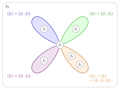
Figure 261: The cyclic subgroups of \(S_3\), drawn inside it. Each petal is the set of powers of one element. The identity \(f_1\), where the petals meet, is in every one, and it is the only element any two of them share. The three swaps \(f_2\), \(f_3\), \(f_4\) each generate a subgroup of two elements, because a swap done twice changes nothing. \(f_5\) and \(f_6\) move all three numbers round and are each other’s inverses, so they generate the same subgroup \({f_1, f_5, f_6}\). No petal is the whole of \(S_3\), so no element generates it and \(S_3\) is not cyclic.
None of the six is all of \(S_3\), so \(S_3\) is not cyclic. It could not have been: every cyclic group is abelian, and \(S_3\) is not (subgroups-and-cyclic-groups). \(\{f_1, f_5, f_6\}\) also shows up as a block of the table when its elements are listed first (cayley-tables).
Common mistakes
- Composing in the wrong order. \(f \circ g\) means \(g\) first. Reading it left to right gives the other product, which in \(S_3\) is usually a different element.
- Reading the table as column \(\circ\) row.
- Thinking \(S_3\) has three elements. It has six. The 3 is the size of the set being rearranged.
- Treating the elements as numbers. \(f_2\) is a function. \(f_2 \circ f_3\) is a composition, not a multiplication of 2 and 3.
- Reading \(f^{-1}\) as \(\frac1f\). It is the inverse function.
- Concluding from “non-abelian” that no two elements commute.
See also
- [groups] — the definition, and abelian against non-abelian
- cayley-tables — reading a table, and why its rows and columns have no repeats
- composition-of-functions — the operation of \(S_n\), and why it is done right to left
- one-to-one-and-onto-functions · inverse-functions — bijections and their inverses, the elements of \(S_n\) and their group inverses
- functions-on-general-sets — a function as a set of pairs
- subgroups-and-cyclic-groups — powers, cyclic subgroups, and why a non-abelian group cannot be cyclic
- 2026-09-24-definitions-and-examples-of-groups — Lecture 26 · 2026-10-06-elementary-properties-of-groups — Lecture 27
- practice-problems — §33, with full worked solutions
Trees
A tree is a connected graph with no non-trivial circuits. Trees are the connected graphs with as few edges as possible, and the circuit-free graphs with as many edges as possible, and the two facts meet in one theorem: a graph with \(n\) vertices is a tree exactly when it is simple, connected and has \(n - 1\) edges. With the Handshake Theorem (graphs) that theorem turns questions about the degrees in a tree into equations. Walks, trails, circuits and connectedness are in walks-trails-and-circuits. First met in 2026-10-29-trees, which has the full proofs and the 11 trees with 7 vertices.
Circuit-free graphs
A circuit is a trail that ends where it starts (walks-trails-and-circuits). A single vertex with no edges counts as one.
A trivial circuit is a circuit consisting of a single vertex and no edges. A non-trivial circuit is a circuit that has edges.
A graph is circuit-free if there are no non-trivial circuits.
Every vertex is a trivial circuit, so the definition has to say non-trivial: otherwise no graph would be circuit-free.
Every circuit-free graph is simple. A loop \(e\) at \(v\) is the non-trivial circuit \(v\,e\,v\). Two edges \(e_1 \neq e_2\) joining \(u\) and \(v\) make the non-trivial circuit \(u\,e_1\,v\,e_2\,u\). So a circuit-free graph has neither (graphs).
Trees
Definition. A graph is a tree if and only if it is connected and circuit-free.
- A single vertex is a tree. So is a single edge, and so is a line of vertices.
- A triangle is not a tree: it is a circuit.
- Two edges with no vertex in common are not a tree: the graph is not connected.
- Every tree is simple, since it is circuit-free.
Small trees
Counting trees means counting essentially different ones: two trees count as the same if one becomes the other by renaming its vertices (they are isomorphic). Up to renaming there is 1 tree with each of 1, 2 and 3 vertices, 2 with 4 vertices, 3 with 5, 6 with 6 and 11 with 7. The 11 are drawn and checked in 2026-10-29-trees.
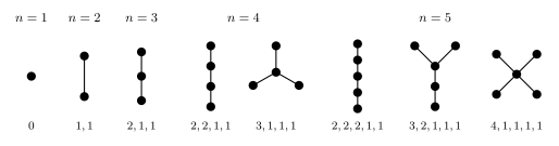
Figure 262: Every tree with 1 to 5 vertices, up to renaming the vertices, each labelled with its degree sequence. With 4 vertices there are two: a line, and one vertex joined to the other three. With 5 there are three: a line, a vertex of degree 3 with one of its branches two long, and one vertex joined to the other four. Each tree with \(n\) vertices has \(n - 1\) edges, and each with at least 2 vertices has at least two vertices of degree 1.
Deleting an edge
If any edge is deleted from a tree then the result is a disconnected graph. This disconnected graph consists of two trees.
Say the edge \(e\) joins \(u\) and \(v\). If \(u\) could still reach \(v\) without \(e\), a shortest such route repeats no vertex, and together with \(e\) it would be a non-trivial circuit in the tree. So nothing joins the side of \(u\) to the side of \(v\), and every vertex is on one side or the other, because its route to \(u\) in the tree either avoids \(e\) or ends by crossing \(e\) from \(v\). Each side is connected, and has no circuit since the tree has none, so each side is a tree. The careful proof is in 2026-10-29-trees.
Minimally connected, maximally circuit-free
A tree sits exactly on the line between too few edges and too many.
- Remove any edge and it is no longer connected. That is the last section. Conversely, a connected graph in which every edge disconnects it when deleted is a tree: if it had a non-trivial circuit, deleting an edge of that circuit would leave it connected, since the rest of the circuit still joins the edge’s two endpoints.
- Add any edge and it gets a circuit. A new loop is a circuit on its own. A new edge \(f\) joining two different vertices \(x\) and \(y\): the tree is connected, so there is a walk from \(x\) to \(y\), and a shortest one never repeats a vertex, so it is a trail. That trail followed by \(f\) back to \(x\) is a non-trivial circuit. Conversely, a circuit-free graph in which every new edge makes a circuit is connected: if \(x\) could not reach \(y\), add a new edge \(f\) joining them. Any circuit it creates must use \(f\), since the graph had none before, and the rest of that circuit would be a walk from \(y\) to \(x\) in the old graph. So no circuit is created.
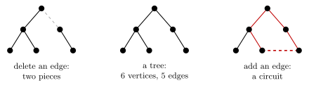
Figure 263: A tree with 6 vertices and 5 edges, in the middle. Left: deleting any one edge, here the dashed one, leaves two pieces with no walk between them, so a tree has no edge to spare. Right: adding any edge, here the dashed red one, closes a non-trivial circuit, in red, so a tree has no room for another edge. 5 edges is the only number of edges a tree with 6 vertices can have.
A tree with \(n\) vertices has \(n - 1\) edges
Theorem. A graph \(G\) with \(n\) vertices is a tree if and only if it is simple, connected and has \(n - 1\) edges.
(\(\Rightarrow\)) A tree is connected by definition and simple because it is circuit-free. For the edges, use strong induction on \(n\). One vertex: no edges, since an edge would be a loop, which is a circuit. For a tree \(T\) with \(k + 1 \geq 2\) vertices, delete any edge. That leaves two trees with \(p\) and \(q\) vertices, where \(p + q = k + 1\) and \(1 \leq p, q \leq k\). By the inductive hypothesis they have \(p - 1\) and \(q - 1\) edges, so \(T\) has \((p - 1) + (q - 1) + 1 = p + q - 1 = k\) edges. The induction is strong because \(p\) and \(q\) can be any sizes below \(k + 1\).
(\(\Leftarrow\)) Let \(G\) be simple and connected with \(n\) vertices and \(n - 1\) edges, and suppose it has a non-trivial circuit. Deleting an edge of a circuit keeps a graph connected, because the rest of the circuit still joins that edge’s endpoints. Keep deleting edges of circuits until none is left. The result is connected and circuit-free, a tree with \(n\) vertices and at most \(n - 2\) edges, which contradicts (\(\Rightarrow\)). So \(G\) has no non-trivial circuit, and is a tree.
Both directions written out in full, with the two facts about deleting edges proved, are in 2026-10-29-trees.
Two consequences:
- Simple is automatic. The proof of (\(\Leftarrow\)) never uses it: any connected graph with \(n\) vertices and \(n - 1\) edges is a tree.
- Connected is not. A triangle together with one more vertex on its own has 4 vertices and 3 edges, and is not a tree. To use the theorem in the (\(\Leftarrow\)) direction, check connectedness.
Vertices of degree 1
A leaf is a vertex of degree 1.
Leaf is the standard word, and it appears in the practice problems, but results in this course are stated as “vertex of degree 1”. In an exam answer, say “vertex of degree 1”, or define leaf before using it.
Theorem. Every tree with at least two vertices has at least two vertices of degree 1.
Proof (handshake). Let \(T\) have \(n \geq 2\) vertices. It has \(n - 1\) edges, so its degrees add to \(2n - 2\). It is connected with at least two vertices, so no vertex has degree 0. If at most one vertex had degree 1, all the others would have degree at least 2, and the degrees would add to at least \(1 + 2(n - 1) = 2n - 1 > 2n - 2\). \(\square\)
Proof (longest walk). Among the walks in \(T\) that visit no vertex twice, take one with the most edges, \(w_0\, f_1\, w_1 \cdots f_k\, w_k\). \(T\) is connected with at least two vertices, so it has an edge, and \(k \geq 1\). Suppose \(w_0\) had another edge \(f \neq f_1\), joining it to \(x\) (\(f\) is not a loop, since \(T\) is simple). If \(x\) is not on the walk, \(x\, f\, w_0\, f_1 \cdots w_k\) is longer and still visits no vertex twice. If \(x = w_j\), then \(w_0\, f_1 \cdots f_j\, w_j\, f\, w_0\) is a non-trivial circuit: its edges are all different, since \(f \neq f_1\) and no other \(f_i\) meets \(w_0\). Both are impossible, so \(\deg(w_0) = 1\), and likewise \(\deg(w_k) = 1\). \(\square\)
The full proof by contradiction is worked in 2026-10-29-trees.
- “At least two vertices” is needed. The tree with one vertex has no vertex of degree 1: its only vertex has degree 0.
- “Two” cannot be improved. A line of vertices has exactly two vertices of degree 1, its ends.
How many vertices of degree 1. Subtract 2 from every degree. In a tree with \(n \geq 2\) vertices the total is \((2n - 2) - 2n = -2\). A vertex of degree 1 gives \(-1\), a vertex of degree 2 gives 0, and every other vertex gives \(\deg(v) - 2 > 0\). So
\[\text{number of vertices of degree 1} \;=\; 2 + \sum_{\deg(v) \geq 3} \big(\deg(v) - 2\big).\]
Every vertex of degree 3 adds one more vertex of degree 1, every vertex of degree 4 adds two, and vertices of degree 2 add nothing. A tree whose other vertices all have degree 2 is a line, with exactly 2.
Counting with the Handshake Theorem
Most questions about trees give some of the degrees and ask for a count. Two facts settle them:
- The theorem: a tree with \(n\) vertices has \(n - 1\) edges.
- The Handshake Theorem: the degrees add to twice the number of edges, so in a tree they add to \(2(n - 1)\).
The method:
- Name the unknown count, \(x\).
- Write the number of vertices \(n\) in terms of \(x\).
- Write the number of edges as \(n - 1\).
- Write the degree sum two ways, from the degrees and as \(2(n - 1)\), and set them equal.
- Solve, then check that the degrees add to twice the edges.
Two more facts often finish the job: every vertex of a tree with at least two vertices has degree at least 1, and there are at least two of degree 1.
Worked: degrees 4, 3 and 1
A tree has three vertices of degree 4, two vertices of degree 3, and every other vertex has degree 1. How many vertices does it have?
Let \(x\) be the number of vertices of degree 1. Then \(n = x + 5\), and the tree has \(n - 1 = x + 4\) edges. The degree sum is
\[3 \cdot 4 + 2 \cdot 3 + x = 2(x + 4), \qquad 18 + x = 2x + 8, \qquad x = 10.\]
So the tree has \(n = 15\) vertices. Check: \(12 + 6 + 10 = 28 = 2 \cdot 14\), and \(14 = 15 - 1\). The formula for vertices of degree 1 agrees: \(2 + 3 \cdot (4 - 2) + 2 \cdot (3 - 2) = 10\).
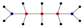
Figure 264: A tree with three vertices of degree 4, in red, two of degree 3, in blue, and every other vertex of degree 1. The red vertices lie in a line, each blue vertex hangs off an end of it, and each of the five has two vertices of degree 1 joined to it. That is \(5 + 10 = 15\) vertices and 14 edges, and the degrees add to \(12 + 6 + 10 = 28 = 2 \cdot 14\).
More worked examples, with figures: 2026-10-29-trees (every degree 3 or 1, with 15 edges) and 2026-10-29-trees (two of degree 4, one of degree 2).
Common mistakes
- Using \(n - 1\) edges for a graph that is not a tree. The count needs connected and circuit-free. In the other direction, \(n - 1\) edges alone is not enough: a triangle and a separate vertex have 4 vertices and 3 edges.
- Off by one. \(n\) vertices go with \(n - 1\) edges, so 15 edges means 16 vertices, not 14.
- Miscounting the vertices. If \(x\) is the number of vertices of degree 1 and three other vertices are named, there are \(x + 3\) vertices, not \(x\).
- Forgetting why no degree is 0. In a tree with at least two vertices every vertex has degree at least 1 because the tree is connected. Say so: the bounds on the degree sum depend on it.
- Calling a single vertex a leaf. The one-vertex tree has a vertex of degree 0 and no vertex of degree 1. The two-leaves theorem needs at least two vertices.
- Deleting an edge from any graph and expecting two pieces. That is true for trees. An edge on a circuit can be deleted without disconnecting anything.
- Reading “circuit-free” as “no circuits at all”. Every vertex is a trivial circuit. Circuit-free means no circuit with edges.
- Judging two trees by their degree sequences. Different degree sequences mean different trees, but the same degree sequence does not mean the same tree: with 7 vertices, three different trees all have degrees \(3, 2, 2, 2, 1, 1, 1\) (2026-10-29-trees).
See also
- walks-trails-and-circuits — circuits, trails and walks, and connected graphs
- graphs — the degrees add to twice the number of edges
- strong-induction-and-the-well-ordering-principle — the induction behind the \(n - 1\) theorem
- proof-techniques — proof by contradiction, used for (\(\Leftarrow\)) and for the vertices of degree 1
- 2026-10-29-trees — Lecture 36, with the full proofs and the 11 trees with 7 vertices
- practice-problems — §46, with full worked solutions
Valid Argument Forms
An argument is a sequence of statements: one or more premises, followed by a conclusion. An argument is valid if whenever all the premises are true, the conclusion is also true — equivalently, if
\[(\text{Premise}_1 \land \text{Premise}_2 \land \cdots \land \text{Premise}_n) \to \text{Conclusion}\]
is a tautology.
Validity is about the argument’s form, not the truth of its statements: an argument can be valid with a false premise or a false conclusion. It can also have true premises and a true conclusion and still be invalid, if the truth of the conclusion doesn’t actually follow from the premises.
Provided in the exam. The named forms below are on the MATH1061/MATH7861 Examination Formula Page, alongside the logical-equivalence-laws. The rules of inference do not have to be memorised; the work left is recognising a form and naming it.
How an argument is written down
The course lays an argument out with the premises stacked one per line and left-aligned, numbered 1. 2. 3., and the conclusion on the last line prefixed by \(\therefore\) (“therefore”) and left unnumbered. There is no horizontal rule above the conclusion:
\[ \begin{aligned} &1. \quad p \to q \\ &2. \quad p \\ &\therefore \quad q \end{aligned} \]
The premise numbers are not decoration — they are what the justification column of a rules-of-inference proof refers back to (“from 1 and 4, by transitivity”).
Why a false premise never threatens validity
In any row of the truth table where at least one premise is false, the conjunction of the premises is false — and \(\text{F} \to X\) is true whatever \(X\) is. So that row of \((\text{Premise}_1 \land \cdots \land \text{Premise}_n) \to \text{Conclusion}\) is automatically T, no matter what the conclusion does there.
This is why the truth table method only inspects the rows where all premises are true: those are the only rows that can make the conditional false. It does not mean an argument with a false premise is automatically valid — a tautology needs every row true, and the all-premises-true rows still have to be checked.
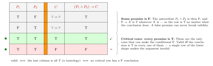
Figure 265: The definition of validity as a picture of a truth table. Rows where some premise is false (grey) make the antecedent of the packaged conditional false, so they are true for free and cannot break the tautology — which is why a false premise never threatens validity. Only the critical rows (starred, all premises T) decide the question. The amber band separates the premises from the conclusion. The red row is the one shape that would make an argument invalid.
Determining validity
- Truth table method: build a truth table for the premises and the conclusion. The argument is valid iff every row where all premises are T also has the conclusion T. Mark the all-premises-true rows with a \(\bigstar\) in the margin and tick the conclusion in those rows, so the check is visible on the page.
- Rules of inference method: chain the laws of logical equivalence (see logical-equivalence-laws) and the valid argument forms below to derive the conclusion from the premises. This proves validity; it can never prove invalidity — failing to find a derivation is not evidence there isn’t one.
- Invalidity method: assume all the premises are true and the conclusion is false, then reason out what that assumption forces each variable to be. Reaching a contradiction (some variable forced to be both T and F) means the assumption was impossible — the argument is valid. Reaching a consistent assignment instead gives a counterexample — the argument is invalid. This directed search is usually faster than building the full truth table once there are 3+ variables, and it is the only one of the three that hands you the counterexample when the argument fails.
Writing up a rules-of-inference proof
The layout is three columns: the line number down the left, the derived statement in the middle, and the justification in its own right-hand column — naming the law or form applied, and usually the lines it draws on (line 4 below is a step that names no line):
| statement | justification | |
|---|---|---|
| 1. | \(w \to b\) | premise 1 |
| 2. | \(d \to \sim b\) | premise 2 |
| 3. | \(\sim(\sim b) \to \sim d\) | from 2, by contrapositive |
| 4. | \(b \to \sim d\) | by the double negative law |
The last column is not optional: the explanations must be written. A chain of correct lines with no justifications is not a proof in this course.
Two rewrites that do most of the work
\[p \to q \;\equiv\; \sim p \lor q \;\equiv\; \sim q \to \sim p\]
Each has a name: \(\sim p \lor q\) is the definition of \(\to\), and \(\sim q \to \sim p\) is the contrapositive. Between them they are what lets a conditional premise be turned into a disjunction (to reach a disjunctive conclusion) or flipped end-for-end (to line up with another conditional for Transitivity). Both are cited by name in the proof started above (in full in determining-argument-validity) — the contrapositive at line 3, the definition of \(\to\) at line 6 — though they are far from the only justifications a proof uses. See conditional-statements.
Valid argument forms
| Name | Form(s) |
|---|---|
| Modus Ponens | \(p \to q,\ p\ \therefore q\) |
| Modus Tollens | \(p \to q,\ \sim q\ \therefore \sim p\) |
| Generalization | (a) \(p\ \therefore p \lor q\); (b) \(q\ \therefore p \lor q\) |
| Specialization | (a) \(p \land q\ \therefore p\); (b) \(p \land q\ \therefore q\) |
| Conjunction | \(p,\ q\ \therefore p \land q\) |
| Elimination | (a) \(p \lor q,\ \sim q\ \therefore p\); (b) \(p \lor q,\ \sim p\ \therefore q\) |
| Transitivity | \(p \to q,\ q \to r\ \therefore p \to r\) |
| Proof by division into cases | \(p \lor q,\ p \to r,\ q \to r\ \therefore r\) |
| Contradiction Rule | \(\sim p \to \mathbf{c}\ \therefore p\) |
These don’t need to be memorised. Treat the table as a reference to scan rather than a checklist to recite: look down it for a form whose conclusion is the shape you want, then work out what the premises have to be turned into to fire it.
See also
- determining-argument-validity — every Lecture 4 argument worked through, by all three methods
- logical-equivalence-laws
- conditional-statements
- 2026-08-03-valid-and-invalid-arguments — Lecture 4
- practice-problems — §4 Valid and Invalid Arguments, with full worked solutions
Walks, Trails and Circuits
A walk is a way of getting around a graph: start at a vertex and keep moving along edges. A trail is a walk that never uses an edge twice, and a circuit is a trail that finishes where it started. The difference that matters is edges versus vertices: a trail may come back to a vertex it has already visited, as long as it leaves along a new edge. The last definition here, connected, says that a walk can get from any vertex to any other. These words are what euler-circuits-and-trails and [trees] are built from. Graphs, degree and the rest of the basic vocabulary are in [graphs]. First met in 2026-10-26-walks-trails-and-circuits.
Walks
A walk is a sequence \[v_0\, e_1\, v_1\, e_2\, v_2 \cdots v_{i-1}\, e_i\, v_i \cdots e_{n-1}\, v_{n-1}\, e_n\, v_n\] where each \(v_i\) is a vertex, and each \(e_i\) is an edge with endpoints \(v_{i-1}\) and \(v_i\).
It alternates vertex, edge, vertex, edge, …, and starts and ends with a vertex. Each edge joins the vertex before it to the vertex after it. This is a walk from \(v_0\) to \(v_n\), and it has \(n\) edges, counted with repeats.
- Anything can repeat. A walk can go back along the edge it just used, and pass through the same vertex many times.
- A walk can have no edges. With \(n = 0\) the walk is the single vertex \(v_0\). That is a walk from \(v_0\) to itself.
- A loop can be used. If \(e\) is a loop at \(v\), its endpoints are \(v\) and \(v\), so \(v\, e\, v\) is a walk.
- Why the edges are written in. If two vertices are joined by multiple edges, the vertices alone do not say which edge was used. In a simple graph two vertices are joined by at most one edge (graphs), so the vertices determine the edges and a walk can be written \(v_0 v_1 \cdots v_n\), or \(a, b, c, \dots\).
Trails
A trail is a walk where \(e_1, e_2, \dots, e_n\) are pairwise distinct.
No edge is used twice. That is the only condition. Vertices may repeat: a trail can come back to a vertex it has visited before, provided it arrives and leaves along edges it has not used yet. Every trail is a walk; a walk that uses some edge twice is not a trail.
Circuits
A circuit is a trail \(v_0\, e_1\, v_1\, e_2 \cdots v_{n-1}\, e_n\, v_n\) where \(v_0 = v_n\).
A circuit is a trail that finishes where it started. Like any trail it uses no edge twice, and it can pass through other vertices more than once.
A trivial circuit is a circuit consisting of a single vertex and no edges.
A non-trivial circuit is a circuit that has edges.
A graph is circuit-free if there are no non-trivial circuits.
Every vertex \(v\) gives a trivial circuit, the walk \(v\) with \(n = 0\): it is a trail (it has no edges to repeat) and it starts and ends at \(v\). Every graph has these, so “circuit-free” has to mean free of the non-trivial ones.
The smallest non-trivial circuits:
- One edge: a loop \(e\) at \(v\) gives the circuit \(v\, e\, v\). An ordinary edge \(e\) joining \(v\) and \(w\) does not give one, because \(v\, e\, w\, e\, v\) uses \(e\) twice.
- Two edges: two edges \(e_1, e_2\) that both join \(v\) and \(w\) give the circuit \(v\, e_1\, w\, e_2\, v\).
- In a simple graph there are no loops and no multiple edges, so a non-trivial circuit has at least 3 edges. A triangle \(a\, b\, c\, a\) is the smallest.
| Edge repeated? | Vertex repeated? | Ends where it starts? | |
|---|---|---|---|
| Walk | allowed | allowed | allowed, not required |
| Trail | no | allowed | allowed, not required |
| Circuit | no | allowed | yes |
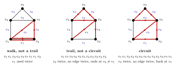
Figure 266: The three definitions on one graph, with the route in red and arrows showing the direction of travel. Left: a walk that is not a trail, since it uses \(e_1\) twice, drawn as the doubled red line. Middle: a trail that is not a circuit. It visits \(v_3\) twice, arriving along \(e_7\) and \(e_3\) and leaving along \(e_6\) and \(e_2\), but uses every edge at most once, and it ends at \(v_2\), not at \(v_1\) where it started. Right: a circuit. It also passes through \(v_3\) twice, uses no edge twice, and returns to \(v_1\).
Two things about circuits used later, in the proofs in euler-circuits-and-trails:
- A circuit can be started anywhere on it. If \(v_0\, e_1\, v_1 \cdots e_n\, v_n\) is a circuit and \(1 \le k \le n\), then \[v_k\, e_{k+1}\, v_{k+1} \cdots e_n\, v_n\, e_1\, v_1 \cdots e_k\, v_k\] is a circuit too. Since \(v_n = v_0\), each edge still joins the vertices beside it, it uses the same edges, and it starts and ends at \(v_k\).
- A circuit can be read backwards. \(v_n\, e_n\, v_{n-1} \cdots e_1\, v_0\) is a circuit with the same edges.
Connected
A graph is connected if and only if there is a walk from any given vertex to any other given vertex.
A graph that is not connected is disconnected: there are two vertices with no walk from one to the other. A drawing of a disconnected graph falls into separate pieces with no edge between them.
- A graph with one vertex is connected. There is no other vertex to reach.
- An isolated vertex disconnects a graph with two or more vertices. A walk from it would have to start along an edge, and it has none.
- A crossing in a drawing is not a connection. Two lines that cross without a dot do not meet, so a drawing that looks like one piece can be a disconnected graph.
To check, pick a vertex, mark every vertex that can be reached from it along edges, then everything reachable from those, and so on. The graph is connected exactly when every vertex ends up marked.
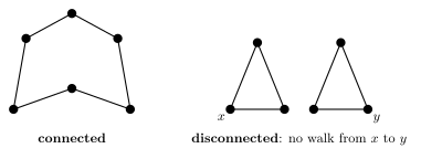
Figure 267: Two graphs with the same degrees, six vertices of degree 2 each. Left: one circuit through all six vertices, a connected graph, since from any vertex there is a walk to any other around the circuit. Right: two separate triangles, a disconnected graph. There is no walk from \(x\) to \(y\), since every walk from \(x\) stays inside its triangle. So the degrees alone do not decide whether a graph is connected.
Common mistakes
- Thinking a trail cannot revisit a vertex. A trail can pass through a vertex as often as it likes. It is the edges that may not repeat.
- Thinking a circuit cannot revisit a vertex. Same again: the circuit in the figure above passes through \(v_3\) twice.
- Going out and back along one edge and calling it a circuit. \(v\, e\, w\, e\, v\) ends where it starts, but uses \(e\) twice, so it is not a trail and not a circuit. It is only a walk.
- Forgetting the trivial circuit. A single vertex with no edges is a circuit. That is why circuit-free is defined by having no non-trivial circuits.
- Reading a crossing as a vertex. Only dots are vertices, so lines that cross do not join two pieces of a graph.
See also
- [graphs] — graphs, loops, multiple edges, simple graphs and degree
- euler-circuits-and-trails — a circuit or trail that uses every edge exactly once
- [trees] — connected, circuit-free graphs
- 2026-10-26-walks-trails-and-circuits — Lecture 34, where these definitions are introduced
- practice-problems — §44, with full worked solutions