Incidence Matrices
An incidence matrix writes a graph down by vertices against edges: a row for each vertex, a column for each edge, and in each place the number of times that vertex is incident with that edge. Each column is one edge, so the matrix is in effect the table of endpoints written as numbers. It has a simple shape that makes it easy to check: every column adds to 2, because every edge has two ends, and every row adds to the degree of its vertex. Putting those together proves the Handshake Theorem again. The other matrix of a graph, vertices against vertices, is in adjacency-matrices. Graphs, loops, degree and the Handshake Theorem are in graphs. First met in 2026-10-27-matrix-representations-of-graphs.
Definition
The incidence matrix of a graph with vertices \(v_1, v_2, \dots, v_n\) and edges \(e_1, e_2, \dots, e_m\) is the \(n \times m\) matrix \(N = [n_{ij}]\) where each entry \(n_{ij}\) is the number of times vertex \(v_i\) is incident with edge \(e_j\).
Rows are vertices and columns are edges. The entry \(n_{ij}\) is about vertex \(v_i\) and edge \(e_j\), in that order, and the first index is the row. The matrix is \(n \times m\): as many rows as vertices, as many columns as edges. Swapping the roles gives the transpose \(N^{\mathsf T}\), which holds the same information but is not the incidence matrix as this course defines it, so write the vertices down the side and the edges across the top, and label both. Like the adjacency matrix, \(N\) depends on the order chosen for the vertices and for the edges.
An edge has two ends. For a vertex \(v_i\) and an edge \(e_j\) there are three cases:
- \(e_j\) does not have \(v_i\) as an endpoint: \(n_{ij} = 0\).
- \(e_j\) joins \(v_i\) to a different vertex: one end is at \(v_i\), so \(n_{ij} = 1\).
- \(e_j\) is a loop at \(v_i\): both ends are at \(v_i\), so \(n_{ij} = 2\).
So every entry is 0, 1 or 2, and a 2 means a loop.
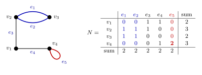
Figure 1: A graph and its incidence matrix, one row for each vertex and one column for each edge. Each column is an edge: e3 has a 1 at each of its endpoints v1 and v2, and the loop e5, in red, has a single 2 at v4, because it meets v4 at both of its ends. The parallel edges e1 and e2, in blue, have the same endpoints and so identical columns. Every column adds to 2, and each row adds to the degree of its vertex: 2, 3, 2, 3.
Columns are edges
The column of \(e_j\) lists how many times each vertex meets \(e_j\). So:
- Every column adds to 2. An edge has exactly two ends, and each end is at one vertex. A column is either two 1s (an edge with two different endpoints, the rows of the 1s) or a single 2 (a loop, at the row of the 2), and 0 everywhere else.
- Parallel edges have identical columns. Two edges with the same endpoints meet every vertex the same number of times. In the figure, \(e_1\) and \(e_2\) are both \((0, 1, 1, 0)\).
- A column is never all zeros, since every edge has at least one endpoint.
Rows are vertices
The row of \(v_i\) lists how many times \(v_i\) meets each edge.
- The row sum is the degree. Adding the row counts the ends of edges at \(v_i\), a loop’s two ends included, which is \(\deg(v_i)\) (graphs). Unlike the adjacency matrix, no correction for loops is needed: the loop’s 2 is already in the row.
- An isolated vertex has a row of zeros. It still gets its row.
The Handshake Theorem again
Add up every entry of \(N\) in two ways.
- Column by column: each of the \(m\) columns adds to 2, so the total is \(2m\).
- Row by row: row \(i\) adds to \(\deg(v_i)\), so the total is \(\deg(v_1) + \cdots + \deg(v_n)\).
The two totals are the same number, so
\[\sum_{i=1}^{n} \deg(v_i) = 2m,\]
which is the Handshake Theorem (graphs). It is the same proof as counting edge ends, with the ends laid out in a table: each entry counts ends of one edge at one vertex. In the figure, the row sums \(2 + 3 + 2 + 3\) and the column sums \(2 + 2 + 2 + 2 + 2\) both come to 10.
Loops
A loop at \(v_i\) is incident with \(v_i\) twice, once at each of its ends, so its column has a 2 in row \(v_i\) and 0 everywhere else. In the figure the loop \(e_5\) is the column \((0, 0, 0, 2)\).
This is what keeps the column sums at 2 and makes the row sums the degrees: the 2 is the loop’s contribution to \(\deg(v_i)\).
The adjacency matrix counts a loop differently. It counts edges, and a loop is one edge, so it puts a 1 on the diagonal (adjacency-matrices). The same loop is a 1 in \(A\) and a 2 in \(N\). A column with a single 1 and nothing else is not a loop. It is not an edge at all, since it has only one end.
Reading a graph off a matrix
Read an incidence matrix one column at a time:
- Draw a dot for each row and label it \(v_1, \dots, v_n\).
- For each column \(e_j\): if it has 1s in rows \(i\) and \(k\), draw an edge \(e_j\) joining \(v_i\) and \(v_k\); if it has a 2 in row \(i\), draw a loop \(e_j\) at \(v_i\).
- Check: every column added to 2, and each vertex’s degree in the drawing is its row sum.
For example,
\[N = \begin{array}{c|ccccc} & e_1 & e_2 & e_3 & e_4 & e_5 \\ \hline v_1 & 1 & 0 & 0 & 2 & 0 \\ v_2 & 1 & 1 & 1 & 0 & 0 \\ v_3 & 0 & 1 & 1 & 0 & 1 \\ v_4 & 0 & 0 & 0 & 0 & 1 \end{array}\]
has every column adding to 2. Column by column: \(e_1\) joins \(v_1\) and \(v_2\); \(e_2\) and \(e_3\) both join \(v_2\) and \(v_3\), identical columns, so they are parallel; \(e_4\) is a loop at \(v_1\); \(e_5\) joins \(v_3\) and \(v_4\).
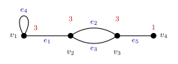
Figure 2: The graph read off the incidence matrix, one column at a time. Columns e2 and e3 are identical, so those two edges are parallel, and column e4 is a single 2 in row v1, so it is a loop at v1. The degrees, in red, are the row sums of the matrix, 3, 3, 3, 1, and they add to 10, twice the 5 edges.
Unlike an adjacency matrix, an incidence matrix names every edge, so the graph comes back with its edge names as well.
Which matrices are incidence matrices
A matrix with at least one row is the incidence matrix of some graph if and only if every entry is a non-negative integer and every column adds to 2. Equivalently, every column is either two 1s and the rest 0, or a single 2 and the rest 0.
The two forms agree: non-negative integers adding to 2 are either \(1 + 1\) or \(2\), with zeros elsewhere.
Proof. (\(\Rightarrow\)) Shown above: each column is an edge, and an edge is two 1s at its two endpoints or a single 2 at the vertex of a loop.
(\(\Leftarrow\)) Let \(M\) be an \(n \times m\) matrix, \(n \ge 1\), whose columns each have one of the two forms. Build a graph with vertices \(v_1, \dots, v_n\) and, for each column \(j\), an edge \(e_j\): if column \(j\) has 1s in rows \(i\) and \(k\), let \(e_j\) join \(v_i\) and \(v_k\); if it has a 2 in row \(i\), let \(e_j\) be a loop at \(v_i\). Then \(v_i\) is incident with \(e_j\) once if \(v_i\) is one of two endpoints, twice if \(e_j\) is a loop at \(v_i\), and not at all otherwise, which is the entry \(m_{ij}\) in every case. So \(M\) is this graph’s incidence matrix. \(\square\)
Only the columns are tested. The rows can be anything, a row of zeros included (an isolated vertex), and the matrix does not have to be square or symmetric. A graph with no edges has no columns at all, and then there is nothing to check.
| Matrix | Column sums | Incidence matrix? |
|---|---|---|
| \(\begin{bmatrix} 1 & 2 \\ 1 & 0 \end{bmatrix}\) | \(2,\ 2\) | yes: an edge \(v_1 v_2\) and a loop at \(v_1\) |
| \(\begin{bmatrix} 1 & 1 \\ 1 & 0 \\ 0 & 0 \end{bmatrix}\) | \(2,\ 1\) | no: the second edge has only one end |
| \(\begin{bmatrix} 1 \\ 1 \\ 1 \end{bmatrix}\) | \(3\) | no: an edge with three ends |
| \(\begin{bmatrix} 0 \\ 2 \\ 0 \end{bmatrix}\) | \(2\) | yes: three vertices, a loop at \(v_2\), and \(v_1\), \(v_3\) isolated |
Four more are worked in 2026-10-27-matrix-representations-of-graphs.
Adjacency and incidence compared
The graph in the figure has both matrices:
\[A = \begin{array}{c|cccc} & v_1 & v_2 & v_3 & v_4 \\ \hline v_1 & 0 & 1 & 0 & 1 \\ v_2 & 1 & 0 & 2 & 0 \\ v_3 & 0 & 2 & 0 & 0 \\ v_4 & 1 & 0 & 0 & 1 \end{array} \qquad\qquad N = \begin{array}{c|ccccc} & e_1 & e_2 & e_3 & e_4 & e_5 \\ \hline v_1 & 0 & 0 & 1 & 1 & 0 \\ v_2 & 1 & 1 & 1 & 0 & 0 \\ v_3 & 1 & 1 & 0 & 0 & 0 \\ v_4 & 0 & 0 & 0 & 1 & 2 \end{array}\]
| Adjacency matrix \(A\) | Incidence matrix \(N\) | |
|---|---|---|
| Size | \(n \times n\) | \(n \times m\) |
| Rows | vertices | vertices |
| Columns | vertices | edges |
| Entry | number of edges with endpoints \(\{v_i, v_j\}\) | number of times \(v_i\) is incident with \(e_j\) |
| Entries can be | any non-negative integer | 0, 1 or 2 |
| A loop at \(v_i\) | 1 on the diagonal, at \(a_{ii}\) | 2 in its column, at row \(v_i\) |
| Parallel edges | one entry bigger than 1 | identical columns |
| Shape | square and symmetric | any; each column adds to 2 |
| \(\deg(v_i)\) | row sum plus \(a_{ii}\) | row sum |
| Number of edges | sum on and above the diagonal | number of columns |
| Edge names | not recorded | one column per named edge |
From \(N\) to \(A\). Off the diagonal, \(a_{ij}\) is the number of columns with a 1 in both row \(i\) and row \(j\). On the diagonal, \(a_{ii}\) is the number of columns with a 2 in row \(i\). In \(N\) above, two columns (\(e_1\) and \(e_2\)) have 1s in rows \(v_2\) and \(v_3\), so \(a_{23} = 2\), and one column (\(e_5\)) has a 2 in row \(v_4\), so \(a_{44} = 1\).
From \(A\) to \(N\), the edges first have to be named, since \(A\) only says how many edges join each pair. Any naming gives an incidence matrix of the same graph, with its columns in a different order.
\(A\) is the more compact when there are many edges. \(N\) is the one to use when the edges themselves matter, as in listing an Euler circuit edge by edge, which is done from an incidence matrix in 2026-10-27-matrix-representations-of-graphs.
Common mistakes
- Swapping rows and columns. In this course the vertices are the rows and the edges are the columns. The transpose has the same information but is not the incidence matrix as defined here.
- Writing 1 for a loop. A loop meets its vertex twice, so it is a 2. A column with a single 1 has only one end and is not an edge.
- Adding a loop correction to the row sum. That is for the adjacency matrix. In \(N\) the row sum already is the degree.
- Checking the rows, or symmetry, instead of the columns. Whether a matrix is an incidence matrix is decided by its columns alone: each must add to 2.
- Leaving out an isolated vertex. Every vertex has a row, even if it is all zeros.
- Leaving off the labels. The matrix depends on the order of the vertices and of the edges.
See also
- adjacency-matrices — the vertex-by-vertex matrix, where a loop counts 1
- graphs — loops, parallel edges, degree and the Handshake Theorem
- euler-circuits-and-trails — the even-degree test for an Euler circuit
- 2026-10-27-matrix-representations-of-graphs — Lecture 35
- practice-problems — §45, with full worked solutions