Probability
When every outcome of a random process is equally likely, the probability of an event is a ratio of two counts: the number of outcomes in the event over the number of outcomes altogether. So probability problems of this kind are counting problems twice over, and every tool of counting-principles and counting-selections applies. This note sets up the language, sample spaces, events and equally likely outcomes, gives the formula, shows how the complement turns “at least one” and “not next to” into something easy, and works two examples through in full. Binomial coefficients, which most of the counts here use, have their own note in binomial-coefficients. First met in 2026-10-19-probability-binomial-coefficients.
Sample spaces and events
- A random process (or experiment) is anything with an outcome that is not known in advance: rolling a die, choosing a committee by lot, shuffling a list of numbers.
- The sample space \(S\) is the set of all possible outcomes.
- An event \(E\) is a subset of the sample space, \(E \subseteq S\). The event happens when the outcome is one of the elements of \(E\).
Rolling one die: \(S = \{1, 2, 3, 4, 5, 6\}\), and “the roll is even” is the event \(E = \{2, 4, 6\}\). An event is a set, so the set operations apply. The complement \(E^c = S - E\) is the event that \(E\) does not happen, here \(\{1, 3, 5\}\), “the roll is odd”.
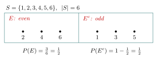
Figure 1: The sample space for one roll of a die, split into the event \(E\), the roll is even, and its complement \(E^c\), the roll is odd. Every outcome lies in exactly one of the two parts. With six equally likely outcomes, \(P(E) = |E| / |S| = 3/6\), and since the two parts fill the whole sample space, \(P(E^c) = 1 - P(E)\).
Equally likely outcomes
If \(S\) is a finite sample space in which every outcome is equally likely, the probability of an event \(E \subseteq S\) is \[P(E) = \frac{|E|}{|S|} = \frac{\text{number of outcomes in } E}{\text{total number of outcomes}}.\]
Wording such as “chosen at random”, “a randomly chosen permutation”, “a fair die” or “shuffled” signals equally likely outcomes. Some consequences come straight from the formula:
- \(0 \le P(E) \le 1\), since \(0 \le |E| \le |S|\).
- \(P(\emptyset) = 0\) and \(P(S) = 1\): an impossible event and a certain one.
- A probability is often quoted as a percentage: \(\frac79 = 0.777\ldots \approx 77.8\%\).
The outcomes must really be equally likely. Roll two dice and ask for the probability that they add to 7. The sums \(2, 3, \dots, 12\) are eleven outcomes, but they are not equally likely, so \(\frac{1}{11}\) is wrong. The equally likely outcomes are the 36 ordered pairs \((1, 1), (1, 2), \dots, (6, 6)\), of which 6 add to 7: \((1,6), (2,5), (3,4), (4,3), (5,2), (6,1)\). So the probability is \(\frac{6}{36} = \frac16\). Choosing a sample space whose outcomes are equally likely is the first step of every problem.
Probability by counting
- Decide what one outcome is, and make sure all outcomes are equally likely. A committee is an unordered selection, a permutation is an ordered arrangement, a password is an ordered selection with repeats (counting-selections).
- Count the sample space, \(|S|\).
- Count the event, \(|E|\), with the same kind of outcome. If \(S\) was counted as unordered selections, \(E\) must be too.
- Divide, and simplify the fraction before turning it into a decimal.
Step 3 is where the counting tools come in: forcing part of the outcome, splitting into categories, gluing objects that must sit together, and the complement.
The complement
For any event \(E\) in a finite sample space \(S\) with equally likely outcomes, \[P(E^c) = 1 - P(E), \qquad\text{equivalently}\qquad P(E) = 1 - P(E^c).\]
Why. \(E\) and \(E^c\) split \(S\) into two disjoint parts, so \(|E^c| = |S| - |E|\) by the difference rule (counting-principles). Dividing by \(|S|\),
\[P(E^c) = \frac{|S| - |E|}{|S|} = 1 - \frac{|E|}{|S|} = 1 - P(E).\]
When to use it. When the event is easier to describe by what it rules out.
- “At least one” has opposite “none”, a single case. \(P(\text{at least one}) = 1 - P(\text{none})\).
- “Not next to each other” has opposite “next to each other”, which is counted by gluing the two objects into one block. \(P(\text{not adjacent}) = 1 - P(\text{adjacent})\).
Worked: a committee with at least one mathematician
A committee of 5 is chosen at random from a group of 25 mathematicians and 25 physicists. What is the probability that at least one mathematician is chosen?
Outcomes. A committee is an unordered selection of 5 of the 50 people, and choosing at random makes every committee equally likely. So
\[|S| = \binom{50}{5} = \frac{50 \cdot 49 \cdot 48 \cdot 47 \cdot 46}{5 \cdot 4 \cdot 3 \cdot 2 \cdot 1} = 2\,118\,760.\]
The complement. “At least one mathematician” means 1, 2, 3, 4 or 5 mathematicians, five cases. Its opposite, “no mathematicians”, is one case: all 5 members are physicists, chosen from the 25 physicists, in
\[\binom{25}{5} = \frac{25 \cdot 24 \cdot 23 \cdot 22 \cdot 21}{5 \cdot 4 \cdot 3 \cdot 2 \cdot 1} = 53\,130\]
ways. Writing \(T = \binom{50}{5}\) for all committees and \(N = \binom{25}{5}\) for those with no mathematicians,
\[\begin{aligned} P(\text{at least one mathematician}) &= \frac{\#(\text{committees with at least one mathematician})}{\#(\text{committees})} = \frac{T - N}{T} = 1 - \frac{N}{T} \\ &= 1 - \frac{\binom{25}{5}}{\binom{50}{5}} = 1 - \frac{53\,130}{2\,118\,760} = 1 - \frac{33}{1316} = \frac{1283}{1316} \\ &\approx 0.9749 \approx 97.5\%. \end{aligned}\]
A quicker route to \(\frac{N}{T}\): the two \(5!\)’s cancel, leaving \(\frac{25 \cdot 24 \cdot 23 \cdot 22 \cdot 21}{50 \cdot 49 \cdot 48 \cdot 47 \cdot 46} = \frac{33}{1316} \approx 0.025\). An all-physicist committee happens about 2.5% of the time.
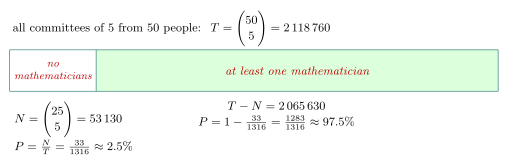
Figure 2: All \(\binom{50}{5}\) committees of 5 drawn from 25 mathematicians and 25 physicists, split by whether they include a mathematician. The two parts are disjoint and fill the whole set, so the shaded event, at least one mathematician, has probability 1 minus the probability of the small part, an all-physicist committee. The widths are not to scale: the all-physicist committees are only about 2.5% of the total.
Worked: 5 not next to 6
What is the probability that a randomly chosen permutation of \(\{1, 2, \dots, 9\}\) has 5 not next to 6?
Outcomes. A permutation is an ordering of all nine numbers: ordered, no repeats. There are \(|S| = 9!\) of them, all equally likely.
The complement. “5 not next to 6” is awkward to count directly, because where 6 may go depends on where 5 is. Its opposite, “5 next to 6”, is easy. If 5 and 6 are adjacent they appear as 56 or as 65.
- Permutations containing 56. Glue 5 and 6 into a single tile 56. Arranging the permutation is now arranging 8 objects, the tile and the other seven numbers, in a row: \(8!\) ways. Each arrangement of the 8 objects gives exactly one permutation of \(\{1, \dots, 9\}\) with 5 immediately before 6, and every such permutation arises once. (Writing it as \(8 \cdot 7!\), with 8 places the tile can start and \(7!\) orders for the rest, gives the same \(8!\).)
- Permutations containing 65. The same argument with the tile 65: \(8!\).
No permutation contains both, so \(2 \cdot 8!\) permutations have 5 next to 6. Then
\[\begin{aligned} P(\text{5 not next to 6}) &= \frac{9! - 2 \cdot 8!}{9!} = 1 - \frac{2 \cdot 8!}{9 \cdot 8!} = 1 - \frac29 \\ &= \frac{9 - 2}{9} = \frac79 = 0.777\ldots \approx 77.8\%. \end{aligned}\]
In numbers, \(9! = 362\,880\) and \(2 \cdot 8! = 80\,640\), so \(282\,240\) permutations have 5 and 6 apart.
A check by positions. Only the positions of 5 and 6 matter. As an unordered pair they are one of \(\binom92 = 36\) equally likely pairs of positions, and 8 of those pairs are adjacent, \(\{1,2\}, \{2,3\}, \dots, \{8,9\}\). So \(P(\text{adjacent}) = \frac{8}{36} = \frac29\), as before.
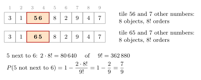
Figure 3: Counting permutations of \(1, \dots, 9\) in which 5 and 6 are next to each other. Glue the pair into one tile. With the tile 56 there are 8 objects to arrange, the tile and the seven other numbers, in \(8!\) ways, and each arrangement unglues to a permutation with 5 just before 6. The tile 65 gives another \(8!\), with 6 just before 5. So \(2 \cdot 8!\) of the \(9!\) permutations have 5 next to 6, and the probability that they are apart is \(1 - \frac{2 \cdot 8!}{9!} = \frac79\).
Common mistakes
- Mixing kinds of outcome. If the sample space counts committees as unordered selections, the event must too. Counting \(|S|\) as \(\binom{50}{5}\) and \(|E|\) as ordered selections gives a “probability” up to \(5! = 120\) times too large, and often bigger than 1.
- Outcomes that aren’t equally likely. The sum of two dice is not uniform on \(2, \dots, 12\); use the 36 ordered pairs.
- Forgetting one of the orders when gluing. “Next to” includes both 56 and 65. Counting only one gives \(P(\text{adjacent}) = \frac19\) and the wrong answer \(\frac89\).
- Labelling the complement as the event. \(\frac{N}{T}\) is the probability of no mathematicians, about 2.5%; \(1 - \frac{N}{T}\) is the probability of at least one, about 97.5%. Name each quantity before computing it.
- Rounding too early. Keep the exact fraction, here \(\frac{1283}{1316}\) and \(\frac79\), and round only at the end.
- A probability outside \([0, 1]\). It always means a slip in one of the counts.
See also
- counting-selections — the four kinds of selection, restrictions, gluing, and counting “at least” through the complement
- counting-principles — the multiplication, addition and difference rules
- binomial-coefficients — \(\binom{n}{r}\), its symmetry and identities
- inclusion-exclusion — counting, and so finding the probability of, a union of events that overlap
- sets-and-set-notation — events are subsets, and \(E^c\) is the set complement
- 2026-10-19-probability-binomial-coefficients — Lecture 31
- practice-problems — §39, with full worked solutions