History of Computing and Foundational Definitions
The course’s opening definitions — what a computer, software, an algorithm, computer science, and software engineering actually are — come with their history. Each is a tentative “perhaps…”, not a formal claim. First met in 2025-07-29-a-brief-history-of-computing.
What is a computer?
A computer is a machine that can carry out sequences of arithmetic or logical operations automatically.
Before it was a machine it was a job title: the Harvard “Computers” of the 1800s were people employed to perform calculations by hand. A photograph of the group shows only women.
The formal definition
A finite state machine is a machine that can change state when given input. A Turing Machine is a finite state machine that additionally has (infinite) read/write memory called tape.
A Turing Machine is a general purpose computer — a single machine that can be programmed to do different tasks, rather than a machine built to do one thing. (Pursued properly in COMP2048, Theory of Computing.)
Alan Turing (1912–1954) gave this formal definition of a computer and of what it means for something to be computable — and in particular demonstrated that there are problems which are not computable. He also played a critical role in breaking the Enigma machine.
A Turing machine that adds two binary numbers makes “changes state when given input” concrete.
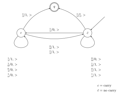
Figure 1: A Turing machine for binary addition. Three states: \(q\), \(c\) = carry and \(\bar c\) = no carry. Every transition is read as what is on the tape / what gets written, which way the head moves: the stacked pair is one bit from each of the two numbers being added, the empty square is a blank cell, and > is a step to the right. The label format, the incoming arrow as the start state, and the double circle on \(q\) as a halting state follow the standard finite-automaton conventions. The transition on a pair of blanks writing 1 appears twice, on both \(c \to q\) and \(c \to \bar c\). The topic belongs to COMP2048.
The labels read as arithmetic. From \(\bar c\), no carry is pending, so \(1 + 1\) writes 0 and moves to \(c\). From \(c\) a carry is pending, so \(1 + 1\) writes 1 and stays in \(c\), while \(0 + 0\) writes 1 and drops back to \(\bar c\). Run off the end of both numbers with a carry still pending and the machine writes the final 1; run off the end without one and it halts leaving the tape alone. It is school-book column addition with the carry held in the state instead of in memory. Two states suffice because a carry is one bit. That is what makes it a usable illustration of “changes state when given input”.
Charles Babbage (1791–1871), an English mathematician, drew the schematics (1840) for the first general purpose computer — the Analytical Engine. It was never built in his lifetime; hardware following the design was assembled in 1910 as a calculator for addition, subtraction, multiplication and division.
The hardware timeline
| Year | Machine | Notes |
|---|---|---|
| 1941 | Z3 | First general purpose computer. Germany, Konrad Zuse. 1 multiplication every 3 seconds. |
| 1945 | ENIAC | Electronic Numerical Integrator and Computer. U. Pennsylvania. $7.3M. 3K instructions/sec. |
| 1949 | EDVAC | Electronic Discrete Variable Automatic Computer. Ballistic Research Laboratory. $1.4M. 340 multiplications/sec. |
| 1951 | UNIVAC 1 | Universal Automatic Computer. Designed for business and admin. $1.8–14M. 2K instructions/sec. |
| 1958 | First integrated circuit | Jack Kilby (Nobel Prize in Physics) — a collection of electronic components fabricated onto silicon. |
| 1962 | UQ’s GE-225 | Installed in the Hawken Building (now the Prentice Centre). Weighed 900kg. |
| 1971 | Intel 4004 | Large scale integration. First commercially produced microprocessor. 92K instructions/sec. |
| 1978 | Intel 8086 | Very large scale integration. 2.5M instructions/sec. |
| 1993 | Pentium | Intel. $1.7K. 188M instructions/sec. |
| — | AMD Ryzen Threadripper 3990x | Ultra large scale integration. $4K. 2.4MM instructions/sec. |
The through-line is integration: a collection of components fabricated onto silicon (1958) → large scale (1971) → very large scale (1978) → ultra large scale (Threadripper).
The speed figures are not in comparable units. Z3 and EDVAC are quoted in multiplications per second, everything else in instructions per second. This is a trend, not a benchmark.
What is software?
Software is the complement of hardware. They are instructions for the machine.
Ada Lovelace (1815–1852), English mathematician and only child of the poet Lord Byron, described an algorithm for the Analytical Engine to compute Bernoulli numbers — she is considered the first computer programmer.
Grace Hopper (1906–1992), a United States Navy rear admiral, pioneered machine independent programming based on English words and invented COBOL. She has both a guided-missile destroyer and a supercomputer named after her.
The “first computer bug” is a moth taped into a 1947 logbook page. The entry, at 15:45 on 9 September, reads:
Relay #70 Panel F (moth) in relay.
First actual case of bug being found.
The page’s other entries — Started Cosine Tape (Sine check), Started Mult+Adder Test — are the ordinary shift log around it. Debugging is routine work, and this is the one entry where the bug was literally an insect.
How do we describe something to a computer?
The earliest answer predates computers entirely: the Jacquard loom used punched cards to control weaving patterns, and punch cards carried programs into machines well into the era of electronic computing. The largest punch card program was 5MB: a shoulder-high bank of loose card stacks.
Above the cards, the same program — integer exponentiation, power(x, y) — walks up through the generations of language:
- Machine code (x86 32-bit): raw bytes,
55/89 E5/B8 01 00 00 00, each one an instruction the CPU decodes directly. The two jumps are a relative jump 9 bytes forward if zero and a relative jump back 11 bytes. - Assembly (1947): the same instructions given mnemonic names and labels —
push ebp,imul eax, ebx,jmp .loop. One line per machine instruction, but readable. - Fortran (1957):
DO 10 I = 1, Y…10 CONTINUE. Numbered statements, but arithmetic looks like arithmetic. - COBOL (1959):
IDENTIFICATION DIVISION.…PERFORM UNTIL COUNTER = 0. Deliberately English-like, designed for business and administration. - C (1972):
for (int i = 0; i < y; i++) { ans = ans * x; }— structured control flow, close to the machine but portable. - Python (1991):
for _ in range(y): ans = ans * x— the loop mechanics disappear entirely.
Each step trades control over the machine for expressiveness to the human. The line count shows it: 19 lines of machine code and 22 of assembly become 5 lines of Python for the same function.
Python
Python was developed by Guido van Rossum and named after the British comedy troupe Monty Python (not the snake). It is a general-purpose, high-level programming language, created to support a variety of programming styles (see programming-paradigms) and to be fun to use.
What is an algorithm?
An algorithm is an ordered sequence of unambiguous instructions that eventually terminates.
The three requirements are each load-bearing: ordered (see the sequencing examples in python-variables-and-memory-model), unambiguous, and eventually terminates — which is exactly what an infinite while True loop fails to do.
The language we use to express an algorithm matters far less than what we are expressing: an instruction sequence that does something useful, like sorting a list. That is why the same exponentiation program above is recognisably the same algorithm in six different languages.
Selection sort on [26, 54, 93, 17, 77, 31, 44, 55, 20] is the example of “something useful”. A nine-row trace shows it with no code, because the code is the part that does not matter yet. The trace is drawn in sorting-algorithms, and selection sort returns in week 13.
What is computer science? What is software engineering?
Computer science is the practice/art of creating algorithms and measuring their relative effectiveness.
Software engineering is the practice/art of creating and maintaining software (realized algorithms) in groups.
The first half of that computer science definition is sorting-algorithms; the second half is algorithmic-complexity. The end of the course does both at once, as a transition from software engineering to computer science.