Algorithmic Complexity (Big-Oh)
An algorithm is an ordered sequence of unambiguous instructions that eventually terminates (see history-of-computing). Once we have more than one algorithm for the same problem, we need a way to say which is better — that measure is complexity.
This is not a side topic bolted on at the end of semester. The entire subject is defined in one sentence:
Computer science is the practice/art of creating algorithms and measuring their relative effectiveness.
First met in lecture 1A. sorting-algorithms is the first half of that sentence; complexity is the second half. The course opens on the definition in week 1 and closes on it in week 13.
Why not just time it?
Timing depends on the machine, the language, what else is running, and the particular input. Instead we count operations. For a sorting algorithm the operations worth counting are comparisons and swaps; more generally we count whatever the algorithm does repeatedly.
The machine matters a great deal. The hardware timeline runs from Konrad Zuse’s Z3 to a current AMD part, and eight of its machines have a quoted speed. Laid on a single logarithmic axis, those speeds are the argument against the stopwatch.
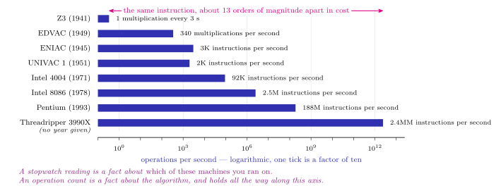
Figure 1: The quoted speeds of the machines in the hardware timeline, on one logarithmic axis. Each bar is one machine. The units are not comparable - Z3 and EDVAC are quoted in multiplications per second and the rest in instructions per second. The rows are not in year order: EDVAC (1949) sits above ENIAC (1945), and the Threadripper has no year. The last figure, 2.4MM, is placed at \(2.4 \times 10^{12}\), reading MM as million-million. The magenta span runs from the slowest machine to the fastest. The full table with prices and manufacturers is in history-of-computing.
Nothing about selection sort changed between 1941 and today. The number of comparisons it makes on a nine-element list is the same on the Z3 as on the Threadripper; only the wall-clock time moves, and it moves by a factor of about \(10^{13}\). That invariant count is what complexity measures.
Definition
We measure the complexity of an algorithm by counting the number of operations performed. But the number of operations is proportional to the length of the input (usually denoted \(n\)) — and it is really this proportion we are interested in, rather than a precise accounting of operations.
That last sentence is the whole idea: 2n + 2 and 5n + 100 are both “linear”, and the difference between them matters far less than the difference between linear and quadratic.
Big-Oh notation
Definition. We say “\(f(n)\) is big-oh of \(g(n)\)”, written \(f(n) = O(g(n))\), when
\[\exists\, c, k \in \mathbb{R}_{>0} : \forall n \geq k,\; 0 \leq f(n) \leq c\,g(n).\]
That is, when there is some positive constant \(c\) such that \(c \cdot g\) is eventually larger than \(f\). The direction matters: “\(f\) is eventually larger than \(cg\)” is backwards and contradicts the inequality.
Worked examples:
- \(2x^2 + x + 1 = O(n^2)\), because for \(x > 2\) we have \(2x^2 + x + 1 < 3x^2\) (take \(c = 3\), \(k = 2\)).
- \(x^3 - \sin(x) = O(n^3)\), because for \(x > 1\) we have \(x^3 - \sin(x) \leq x^3 + 1 < 2x^3\) (take \(c = 2\), \(k = 1\)).
In practice this means: drop the constants and keep only the fastest-growing term.
The four complexity classes in this course
Linear — \(O(n)\)
def linear(xs: list[int]):
    n = len(xs)        # 1  assignment
    index = 0          # 1  assignment
    while index < n:   # n  comparisons
        index += 1     # n  assignments / additions
                       # 2n + 2 = O(n) operations
Quadratic — \(O(n^2)\)
A loop nested inside a loop, each running \(n\) times:
def foo(xs: list[int]):
    n = len(xs)        # 1
    i = 0              # 1
    while i < n:       # n
        j = 0          # n
        while j < n:   # n * n
            j += 1     # n * n
        i += 1         # n
                       # 2n**2 + 3n + 1 = O(n**2)
Constant — \(O(1)\)
The trap here is that a big number is still a constant: the loop below runs ten billion times, but that count does not depend on n at all.
def foo(xs: list[int]):
    n = len(xs)          # 1
    index = 0            # 1
    while i < 10**10:    # 10**10
        index += 1       # 10**10
                         # 2*10**10 + 2 = O(1)
Logarithmic — \(O(\log n)\)
The loop variable is in an exponent, so the loop runs about \(\log_2 n\) times:
def log(xs: list[int]):
    n = len(xs)                # 1
    index = 0                  # 1
    while 2 ** i < len(xs):    # log[2](n)
        i += 1                 # log[2](n)
                               # 2log[2](n) + 2 = O(log(n))
Both this listing and the constant one above mix their counter names: each initialises index and then increments i. Neither would run; the operation counts in the comments are still the point.
The base of the logarithm is a constant factor (\(\log_2 n = \log n / \log 2\)), so it disappears inside the big-oh — \(O(\log_2 n)\) and \(O(\log n)\) mean the same thing.
How to read a loop’s complexity
- A loop that advances by a fixed step toward
n→ \(O(n)\). - A loop that multiplies or divides its counter each pass → \(O(\log n)\).
- Nested loops → multiply their counts (\(O(n) \times O(n) = O(n^2)\)).
- A bound that doesn’t mention
n→ \(O(1)\), however large it is. - A bound that is an input value rather than an input length → see the next section, and be careful.
When the input is a value, not a length
Every example above takes n = len(xs): the input is a collection and \(n\) counts its elements. One of the course’s earliest algorithms, integer division from Lecture 1B, does not fit that mould.
Dividing two integers and still getting an integer is grade-school division: for \(x = 17\) and \(y = 3\), 17 ÷ 3 is 5 remainder 2, i.e.
\[17 = 5 \cdot 3 + 2 \qquad\text{or}\qquad \frac{17}{3} = 5 + \frac{2}{3}.\]
Python hands you both halves directly, and the two together reconstruct the input:
>>> 17 // 3
5
>>> 17 % 3
2
>>> 3 * (17 // 3) + (17 % 3)
17
17 // 3 is the quotient and 17 % 3 is the remainder. The theorem the two operators rest on:
Division algorithm. Let \(x\) and \(y\) be positive integers. There is a unique quotient \(q\) and unique remainder \(r\) with \(0 \le r < y\) satisfying \(x = q\cdot y + r\).
The remainder can also be computed by hand, subtracting y away until nothing more can be taken (while is not taught until week 4):
>>> def remainder(x: int, y: int) -> int:
...     ans = x
...     while ans >= y:
...         ans = ans - y
...     return ans
>>> remainder(17, 7)
3
The recursive version (recursion is week 12, python-recursion):
>>> def remainder(x: int, y: int) -> int:
...     return x if x < y else remainder(x-y, y)
>>> remainder(17, 7)
3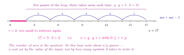
Figure 2: Repeated subtraction for \(17 \div 3\). The number line, the arcs and the count of passes show what the remainder loop does; the equation beneath it is \(17 = 5\cdot 3 + 2\), with the general form \(x = q\cdot y + r\) and \(0 \le r < y\). The code above runs on \((17, 7)\) and the arithmetic on \((17, 3)\); the figure follows the arithmetic.
Now count operations. The loop body runs once per subtraction, and the number of subtractions is exactly \(\lfloor x/y \rfloor\) — the quotient. So remainder(x, y) costs on the order of \(x/y\) operations, and remainder(10**9, 1) would run a billion times while remainder(10, 1) runs ten. The cost is set by the magnitude of the input, not by its length.
That is why complexity is always stated against the size of the input rather than its value. It is also why // and % are worth having: they reach the same two answers without the loop, so the number of subtractions never appears in the running time at all. Whenever you meet a loop whose bound is a number rather than a len, check which of the two kinds you are looking at before naming a complexity class.
Complexity of the sorting algorithms
| Algorithm | Complexity |
|---|---|
| Selection sort | \(O(n^2)\) |
| Insertion sort | \(O(n^2)\) |
| Bubble sort | \(O(n^2)\) |
| Merge sort | \(O(n \ln n)\) |
See sorting-algorithms for how each of these works. Merge sort is written here as \(O(n \ln n)\) — the same class as \(O(n \log n)\), since the base is a constant factor.
Why this matters elsewhere
Complexity is what makes dynamic programming worth doing: a branching recursion like the naive Fibonacci recomputes the same subproblems exponentially many times, and caching collapses that back down to linear. It is also the justification for the dictionary’s “magic” hash function in python-dictionaries — a hash table finds a key in roughly constant time where scanning a list would take linear time.