Complexity and Sorting
See csse1001 for course logistics — this note covers the final lecture’s content. It is numbered Lecture 12B but falls on 28 October, in week 13 of the course profile, paired with the functional programming lecture.
Not testable. The week 13 material is marked “None (not testable)” in the course’s own assessment-coverage schedule. Worth reading for its own sake — and it is the payoff to the definitions in 2025-07-29-a-brief-history-of-computing — but not for exam marks.
Two goals
Sorting a list is a single problem with several different solutions. Five of them are below. Working through them has two goals:
- introduce the notion of an algorithm, and
- formalise how algorithms are compared.
This is part of a transition from software engineering to computer science, and it matches the definition from lecture 1A: computer science is the practice/art of creating algorithms and measuring their relative effectiveness.
The traces and trees below use the layout of the sorting figures at runestone.academy: rows of cells, step captions on the right, and grey shading. This layout matches nothing else in the course (see csse1001-diagram-notation).
The grey shading has no single meaning. Each caption below states what it marks in that particular figure.
Five sorts, five restrictions
Each algorithm is derived by imposing a restriction and asking whether sorting is still possible. See sorting-algorithms for the standalone descriptions.
| Restriction | Algorithm |
|---|---|
| Only select the largest element | Selection sort |
| Only place an element correctly into a sorted list | Insertion sort |
| Only swap adjacent cells | Bubble sort |
| Only merge two sorted lists | Merge sort |
| Only split a list in two by a predicate | Quick sort |
Exercise. Implement selection sort, insertion sort, bubble sort and merge sort.
Selection sort
Suppose we could only select (find the index of) the largest element from a list.
Find the largest member of xs and make it the last element; then find the next largest and make it the second last, and so on.
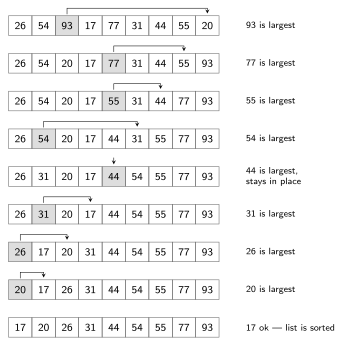
Figure 1: Selection sort on 26 54 93 17 77 31 44 55 20. Time runs downward, one selection per row. The grey cell is the cell being selected on that row: the largest element in the still-unsorted prefix. The arrow above the row shows the long-range swap that sends it to its final position. Each pass shortens the region being searched by one, so the sorted region grows inward from the right — after eight passes the single remaining element (17) is already correct.
Two things the trace makes concrete:
- The invariant is a sorted suffix. Everything at or to the right of each arrowhead is finished and is never touched by a later row; the search region shrinks by one cell per pass.
- A pass whose maximum is already in place still costs a full scan. Row five (“44 is largest, stays in place”) searches the same five-cell region it would have searched anyway and simply performs no swap — selection sort saves nothing from a favourable input.
The starting list differs from every other figure. The selection trace opens on
26 54 93 17 77 31 44 55 20; the insertion, bubble and merge figures all open on54 26 93 17 77 31 44 55 20— the first two elements are transposed. This is a difference between the figures, not a step of the algorithm. Allow for it when comparing the traces row by row.
Insertion sort
Suppose we could only place an element correctly into a sorted list. Could we sort a list?
Sort the list by inserting elements repeatedly into the front of the list. After \(k\) steps the first \(k\) elements of the list will be sorted.
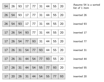
Figure 2: Insertion sort on 54 26 93 17 77 31 44 55 20. Grey marks the sorted prefix, white the untouched tail; each row inserts the leftmost white element into the grey region, so the prefix grows one cell per row. The first row is the base case: a one-element list is already sorted.
Set beside the selection trace, the contrast is the whole point of running both: insertion grows a sorted prefix, selection grows a sorted suffix, and the region insertion has already built keeps being rearranged (inserting 17 shifts three cells right) while selection’s finished suffix is frozen. Insertion also does a variable amount of work per row — inserting 93 costs nothing, inserting 20 shifts seven cells — which is why its behaviour depends on the input in a way selection’s does not.
Bubble sort
Suppose the only operation we could perform on lists was swapping adjacent cells. Could we sort this list?
Pass through the list swapping elements so that larger elements move forward when swapping (for ascending order) — larger elements bubble to the top. Make repeated passes until the list is sorted.
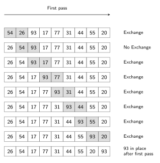
Figure 3: The first pass of bubble sort on 54 26 93 17 77 31 44 55 20. The grey pair is the two adjacent cells being compared on that row; the step caption records whether they were exchanged. The pass makes 8 comparisons and 7 exchanges and ends with 93 — the maximum — parked at the far right. Only the first pass is drawn.
Bubble’s first pass finishes with the maximum where selection’s first pass puts it — parked at the far right — but is only allowed adjacent swaps, so it takes 93 six exchanges to cross the list where selection moved it in one. Only the maximum’s landing place is comparable, mind: the two figures do not start from the same list (see the note above), and everything left of the last cell is in a different order at the end of the two passes. The cost of the restriction is visible directly in the figure: from row three onward 93 steps exactly one cell right per row.
Merge sort
Suppose the only operation we could perform on lists was merging two sorted lists into one sorted list. Could we sort a list?
Break the list in half and sort the halves (using merge sort) then merge these lists. There are two phases: the winding phase, which is the recursive descent, and the unwinding phase, which is the merging on the way back up. This is the winding/unwinding vocabulary from 2025-10-20-recursion.
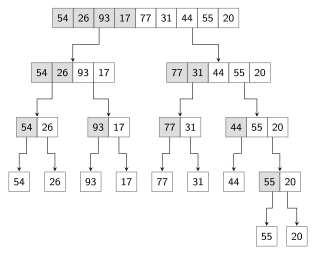
Figure 4: Merge sort winding. The whole list sits at the top and arrows point downward into the two halves of each split; grey marks the left half of every list that is about to be split, so the split point is readable at a glance. Every odd-length row puts the short half first — the nine-element list goes 4/5, not 5/4 — which is why the rightmost branch runs one level deeper than the others.
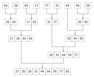
Figure 5: Merge sort unwinding. The singletons are at the top and the sorted list at the bottom; every pair of arrows converges on the merged result. There are two pass-throughs: 44 has no partner at the first merge level and drops straight into 20 44 55, and 31 77 is formed at the first merge level but skips the second, merging only at the third. Both figures use downward arrows — the recursion direction is carried by which end holds the whole list, never by arrow direction.
Read together, the two trees are where merge sort’s better complexity comes from: the winding tree is about \(\log_2 n\) levels deep because each level halves the list, and each level of the unwinding tree touches every element exactly once while merging — depth times work-per-level gives \(n \log n\).
Quick sort
Could we sort a list if all we could do was sort a list into two pieces based on some predicate?
Divide the list into two lists: those bigger than or equal to the head and those less than or equal to the head. Sort those lists and then just connect them.
Which sorting algorithm is best?
Rather than timing, we can count how many times some operations are performed in each sorting algorithm. The operations to count are comparisons and swaps.
Definition (Complexity). We measure the complexity of an algorithm by counting the number of operations performed. However, the number of operations is proportional to the length of the input (usually denoted \(n\)). It is really this proportion we are interested in, rather than a precise accounting of operations.
Big-Oh
Definition (Big-Oh Notation). We say “\(f(n)\) is big-oh of \(g(n)\)” and write \(f(n) = O(g(n))\) when
\[\exists\, c, k \in \mathbb{R}^{>0} : \forall n \geq k;\; 0 \leq f(n) \leq c\,g(n).\]
That is, when there is some positive constant \(c\) such that \(f\) is eventually smaller than \(cg\). Two examples:
- \(2x^2 + x + 1 = O(n^2)\) because for \(x > 2\), \(\;2x^2 + x + 1 < 3x^2\).
- \(x^3 - \sin(x) = O(n^3)\) because for \(x > 1\), \(\;x^3 - \sin(x) \le x^3 + 1 < 2x^3\).
Each example names the witness \(c\) implicitly (3 and 2) and the threshold \(k\) explicitly (2 and 1).
Four worked loops
For each of the four loops below, the complexity of foo comes from counting operations line by line. See algorithmic-complexity for the annotated code of all four.
| Loop shape | Count | Class |
|---|---|---|
while index < n: index += 1 |
\(2n + 2\) | \(O(n)\) Linear |
A while inside a while, both to n |
\(2n^2 + 3n + 1\) | \(O(n^2)\) Quadratic |
while i < 10**10 |
\(2 \cdot 10^{10} + 2\) | \(O(1)\) Constant |
while 2 ** i < n |
\(2\log_2 n + 2\) | \(O(\log n)\) Logarithmic |
The quadratic case is the one that needs its line-by-line working, because it is the only one whose loop lines do not all carry the same count. The other three have two constant assignments and then a matching pair — \(n\) and \(n\), \(10^{10}\) and \(10^{10}\), \(\log_2 n\) and \(\log_2 n\) — whereas this one runs \(n\), \(n \times n\), \(n \times n\), \(n\):
def foo(xs: list[int]):
    n = len(xs)        # 1
    i = 0              # 1
    while i < n:       # n
        j = 0          # n
        while j < n:   # n * n
            j += 1     # n * n
        i += 1         # n
                       # 2n**2 + 3n + 1 = O(n**2)
The body of the outer loop runs \(n\) times, and it contains a loop that runs \(n\) times, so the two inner lines each contribute \(n \times n\). Adding the line counts gives \(1 + 1 + n + n + n^2 + n^2 + n = 2n^2 + 3n + 2\), one more than the \(2n^2 + 3n + 1\) in the table and in the last comment. The constant there is off by one. It makes no difference to the class.
The constant case is the one worth pausing on: ten billion iterations is still \(O(1)\), because the count does not depend on n.
Worked: the complexity of each sorting algorithm
Exercise. Find the complexity of each sorting algorithm.
Answer. Insertion, selection, and bubble are \(O(n^2)\) whereas merge-sort is \(O(n \ln n)\).
| Algorithm | Complexity |
|---|---|
| Insertion, selection, bubble | \(O(n^2)\) |
| Merge sort | \(O(n \ln n)\) |
The logarithm here is \(\ln\), not \(\log_2\) — the base is a constant factor and disappears inside the big-oh either way.
Experimental results
Measured times close the argument. All four algorithms are plotted together first. Merge sort is then replotted alone, because on an axis running to 250 seconds it is indistinguishable from the x-axis.
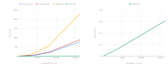
Figure 6: Measured sorting time against list length. Left: all four algorithms on one axis — bubble worst, then insertion, then selection, with merge sort flat on the x-axis. Right: merge sort alone, replotted at roughly 1/300th of the vertical scale. Each quadratic curve roughly quadruples when the list length doubles (bubble 14.9s to 58.2s to 231.2s across n = 4096, 8192, 16384), which is what quadratic growth looks like on a linear axis; merge sort roughly doubles (0.138s to 0.296s to 0.613s). The plotted times and sample lengths are estimates, and the leftmost selection point is interpolated.
At a list of about sixteen thousand elements the separation is roughly 231 s (bubble), 90 s (insertion), 78 s (selection) and 0.6 s (merge) — a factor of nearly 400 between the worst and the best, from algorithm choice alone. The machine, the language and the input used are not known, so take the numbers as one experiment’s shape rather than as a benchmark. This gap is why complexity is worth reasoning about.
The three quadratic sorts also stay within a small constant factor of each other: from about four thousand elements up, bubble runs roughly two and a half times insertion, and insertion a little over selection. The ratio is not fixed all the way down — at the shortest lengths plotted, bubble is under twice insertion — but it is exactly the kind of difference big-oh deliberately throws away. Same class, still very different afternoons.
Previous lecture
2025-10-20-recursion — Lecture 12A. Merge sort and quick sort are both recursive, and the winding/unwinding phases described there are exactly what Figure 4 and Figure 5 show.